Instance reduction for time series classification using MDL principle

Abstract

Research in time series classification has shown that the one nearest neighbor with Dynamic Time Warping measure in most cases outperforms more advanced classification algorithms. Instance reduction is one of the approaches to improve time and space efficiency of nearest neighbor classifier for time series data. This approach reduces the size of the training set by selecting the best representative instances and uses only them during classification of new instances. In this work, we propose a novel approach for instance reduction in time series classification. Our method consists of two steps. First, we remove the unrepresentative instances in the training set, using data editing. In the second step, we compress the training set using the Minimum Description Length principle. The main idea behind our method is that if we can compress the two time series by the Minimum Description Length principle, we will combine them into one time series. By this way, the number of instances in the training set is reduced step by step, and we stop removing instances from the training set when reaching some required percentage of instances in the training set or when we can not find any pair of instances to compress. We empirically compare our proposed method with the two previous methods, INSIGHT and Naïve Rank Reduction, over a vast majority number of time series training sets. The experimental results show that our method can outperform INSIGHT and Naïve Rank Reduction in many datasets when the percentage of selected instances in the training set is not too small, about greater than 30%.

Keywords

Time series classification dynamic time warping instance reduction MDL principle compression rate

1. Introduction

Time series data exists in several applications of our life, in a vast majority of fields such as finance, economy, medicine, environment, government, engineering or industry. There are many time series data mining tasks such as similarity search, motif discovery, anomaly detection, rule extraction, clustering, and classification. Among these tasks, classification problem is a traditional important problem. Time series classification is the theoretical background of many recognition tasks such as signature verification, speech, handwriting recognition. In medicine, time series classification can be applied in the analysis of images, brainwaves (EEG) and electrocardiograph (ECG) signals.

Although there has been much research on classification in general, the most classic machine learning and data mining algorithms do not work well for time series data due to their unique characteristics. In particular, the high dimensionality, very high feature correlation and the large amount of noise that characterize time series present a difficult challenge. There are a few classification methods that can be applied to time series data such as: Artificial Neural Network, Bayesian Network, Decision Tree, k-Nearest Neighbors. Among these methods, the simple approach, 1-Nearest Neighbor Classifier using Dynamic Time Warping (DTW) measure [5, 21] was considered that it is hard to beat [34].

There are four major approaches to enhance the efficiency of 1-Nearest Neighbor Classifier for time series data. One way to speed up 1-Nearest Neighbor Classifier is to use some indexing structures to support time series similarity search such as R-tree [12], R*-tree [3], M-tree [9], TS-tree [1]. A second way to improve the efficiency of 1-Nearest Neighbor Classifier for time series data is to reduce the dimensionality of time series by using some approximation methods such as PAA (Piecewise Aggregate Approximation) [19], PLA (Piecewise Linear Approximation) [20] or to transform into discrete symbols such as SAX (Symbolic Aggregate Approximation) [24]. Another way is to speed up the computation of the DTW distance function. One well-known technique to accelerate the computation of DTW is to use lower bounding techniques [21, 22, 23, 26]. Another direction to improve the efficiency of 1-Nearest Neighbor Classifier is reducing the number of instances in the training set. We can simply discard a fraction of the training data to improve the performance. It is well known that for general instance reduction, if we are careful in selecting which instances we discard, we can significantly reduce the classification time and the storage requirement of the training set while maintaining high accuracy.

For the last direction, while the idea of instance reduction for nearest neighbor classifiers has a long history, surprisingly there have been very few methods of this direction proposed for time series classification. So far, there are two instance reduction methods for time series: Naïve Rank Reduction, was proposed by Xi et al. [38], and INSIGHT, which is based on graph theory, was proposed by Buza et al. [7].

In this work, we propose a novel method to reduce the number of instances in the training set for time series classification which is based on the Minimum Description Length (MDL) principle. MDL has been widely used in bioinformatics, text mining, etc. yet it is still under-explored in time series domains. This is mainly because MDL is defined in discrete space. Some recent publications [14, 27] provide an in-depth analysis of the potential of applying MDL principle to real-valued time series data. Our proposed method, called IR_M (Instance Reduction based on MDL principle), is the first attempt to apply MDL in instance reduction for nearest-neighbor classification of time series. It consists of two steps: removing the unrepresentative instances and compressing the training set. In the first step, we remove the unrepresentative instances in the training set, which are the instances that their nearest neighbors in the training set belong to another class. After the first step, if the number of instances in the training set has not reached the required percentage of instances yet, we continue to the second step which is the main process in our method. In the second step, if any pairs of time series can be compressed by the MDL principle, they will be combined into one time series. Therefore, the number of instances in the training set is reduced step by step, and we stop removing instances when some required percentage of instances in the training set is reached or when we can not find any pair of instances to compress. Besides, we also propose a principled way to automatically determine the point at which the instance removal process should stop. That means our proposed method can be used as parameter-free or parametric.

We empirically compare the IR_M method with the two previous methods INSIGHT [7], and the Naïve Rank Reduction [38] over a collection of 44 publicly available datasets for time series classification. In most of the datasets, the experimental results reveal that IR_M can outperform INSIGHT method and Naïve Rank Reduction when the percentage of selected instances in the training set is not too small, about greater than 30% of the original training set.

The rest of this paper is organized as follows. Section 2 reviews some background on time series data and MDL principle. Section 3 reviews the two previous methods on instance reduction for time series classification. Section 4 gives details of our proposed method, and followed by a set of experiments in Section 5. Section 6 concludes the work and gives suggestions for future works.

2. Backgrounds

In this section, we introduce some background on time series classification, Dynamic Time Warping and the MDL principle for time series data.

2.1 Time series

A time series $T$ is a sequence of real numbers collected at regular intervals over a period of time: $T=t_{1},t_{2},\ldots,t_{n}$ . We are given some groups of time series. These groups are called classes. The class label class( $T$ ) shows the class of time series $T$ .

2.2 1-Nearest Neighbor Classifier

In 1-Nearest Neighbor Classifier (1-NN), the data object is classified to the same class as its nearest object in the training set. The 1-NN combined with DTW has been approved hard-to-beat in classification of time series data among many other methods such as Artificial Neural Network (ANN), Bayesian Network, Decision Tree, etc. [34]. In this work, we use 1-NN to classify time series data and evaluate the error rate of this classifier on the reduced training set.

2.3 Distance measures on time series

Distance measure has a huge impact on several time series data mining tasks such as similarity search, classification, clustering, motif discovery, anomaly detection, rule extraction. All of these problems need a distance measure function to estimate the similarity between time series. There have been several distance functions proposed for time series, among them, Euclidean Distance and Dynamic Time Warping distance are the most widely used.

2.4 Dynamic Time Warping

Dynamic Time Warping (DTW) distance [5] aims to find the best matching between two time series. During that matching, it calculates the smallest distance between two time series. Such a best matching is also called the warping path. However, DTW incurs high computational complexity (i.e., $O(n^{2})$ ). Figure 1 shows the alignment between two time series when we calculate difference values between them. DTW calculates a minimum distance between two time series by finding a warping path which is a non-linear alignment, whereas Euclidean Distance calculates the difference between two time series using a linear alignment. This difference makes DTW much more flexible than Euclidean Distance.

Figure 1.

A comparison of Euclidean Distance (a) and Dynamic Time Warping (b).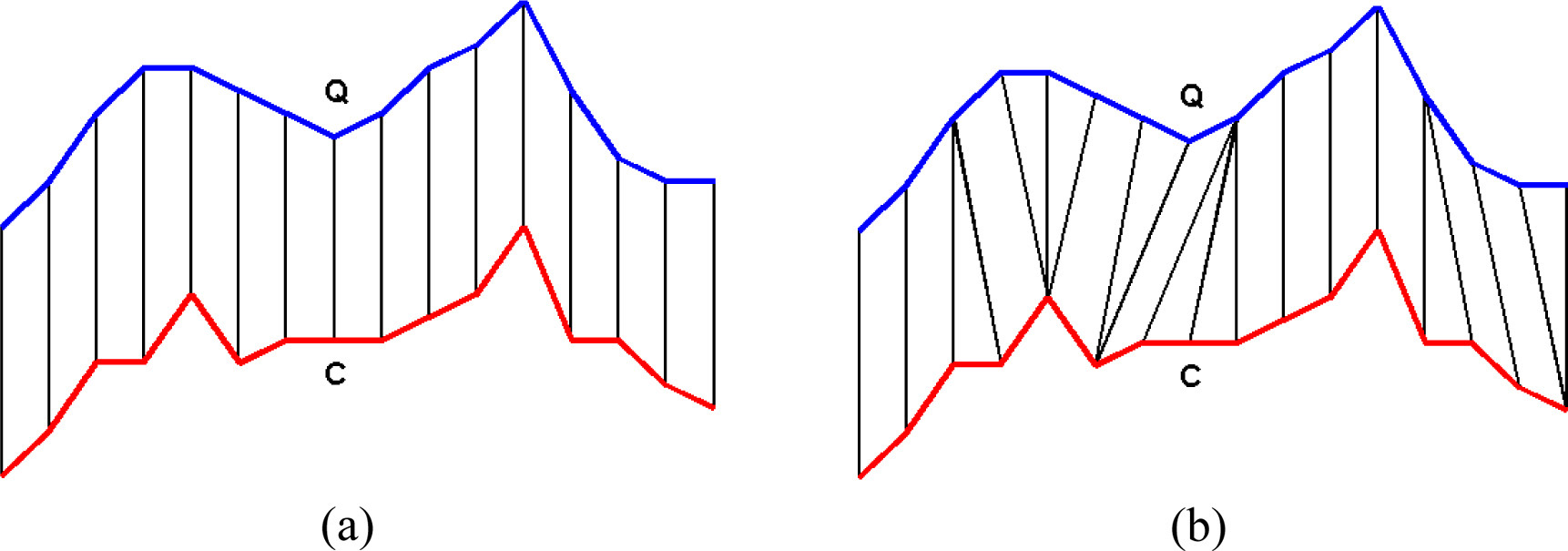

Given two time series $Q$ and $C$ which have length $n$ and $m$ respectively: $Q=q_{1},q_{2},\ldots,q_{n}$ and $C=c_{1},c_{2},\ldots,c_{m}$ . DTW is a dynamic programming technique which calculates all possible warping paths between two time series for finding minimum distance. To calculate DTW between the two above time series, firstly we construct a matrix $D$ with size $m\times n$ . Every element in matrix $D$ is cumulative distance defined as:

$\gamma(i,j)=d(i,j)+\min\{\gamma(i-1,j),\gamma(i,j-1),\gamma(i-1,j-1)\}$

where $\gamma(i,j)$ is $(i,j)$ element of matrix that is a summation between $d(i$ , $j)=$ ( $q_{i}-c_{j})^{2}$ , a square distance of $q_{i}$ and $c_{j}$ , and the minimum cumulative distance of three adjacent elements to $(i,j)$ .

Next, we choose the optimal warping path which has minimum cumulative distance defined as:

$\textit{DTW}(Q,C)=\min\sum\limits_{k=1}^{K}{w_{k}}$

where $w_{k}$ is $(i,j)$ at $k^{\rm th}$ element of the warping path, and $K$ is the length of the warping path.

For a more efficient DTW distance computation, some global constraints were suggested to DTW [15, 29]. A well-known constraint is Sakoe-Chiba band [29]. The Sakoe-Chiba band constrains the indices of the warping path $w_{k}=(i,j)_{k}$ such that $j-r\leqslant i\leqslant j+r$ , where $r$ is a term defining the allowed range of warping, for a given point in a sequence. In this work, we use DTW with Sakoe-Chiba band constraint to evaluate distance between time series in 1-Nearest Neighbor Classifier.

2.5 Minimum Description Length principle: A model selection method

The Minimum Description Length principle is a formalization of Occam’s razor in which the best hypothesis for a given set of data is the one that leads to the best compression of the data. MDL was introduced by Rissanen [28]. This principle is a crucial concept in information theory and computational learning theory.

MDL has had a significant impact in bioinformatics and data mining of discrete objects but has yet failed to have significant impact on real-valued data mining. Recently, there have been some efforts to use MDL principle in time series data mining tasks. Tanaka et al. applied MDL in the EMD algorithm which discovers motifs in time series [31]. The EMD algorithm operates on a quantized representation of the data which has the disadvantages of requiring three parameters (cardinality, dimensionality, and window size). Begum et al. proposed a stopping criterion for semi-supervised time series classification based on MDL [4]. Rakthanmanon et al. developed an MDL-based method for time series clustering [27]. Shokooki-Yekta et al. applied MDL in time series rule discovery [30]. The three latter works follow a new framework of MDL approach which is effective, efficient and more suitable for time series data.

MDL is a principle; this means that there is no “single uniquely optimal MDL method/procedure/ algorithm” [11]. In some special situations, we can distinguish between good and not good versions of MDL principle [11].

In this work, we use a specific version of MDL principle for time series data which was used in some previous studies such as in [4, 27]. We choose this version of MDL principle because it is parameter-free, suitable for time series data, and it allows for a more intuitive explanation of our algorithms.

2.5.1 Discrete normalization function

The MDL technique that is at the heart of our work requires discrete data, but most time series dataset are real-valued. To overcome this problem, we cast the real-valued numbers into a reduced cardinality version by using the following discrete normalization function.

A discrete function Dis_Norm is the function to normalize a real-value subsequence $T$ into $b$ -bit discrete value of range $[1,2^{b}]$ . The maximum of the discrete range value 2 ${}^{b}$ is also called the cardinality. The discrete function is defined as follows:

$\textit{Dis{\_}Norm}(T)={\rm round}[(T-\textit{min})/(\textit{max}-\textit{min% })\times(2^{b}-1)]+1$

where min and max are the minimum and maximum value in $T$ , respectively.

After casting the original real-valued data to discrete values, we are interested in determining how many bits are needed to store a particular time series $T$ . It is called the Description Length of $T$ . There are several ways to approximate the description length of time series, using Huffman coding, Shanon-Fano coding, etc. Since entropy is a lower bound on average code length from any such encoding, we can use the entropy of the time series as its description length.

2.5.2 Entropy

Entropy can be understood as the average number of bits requires representing one element of a sequence. The entropy of a time series $T$ is defined as follows:

$H(T)=-\sum\limits_{t\in\textit{unique}(T)}{P(T=t)\log_{2}P(T=t)}$

where $P(T=t)$ is the probability of value $t$ in time series $T$ , and unique( $T$ ) is a set of unique values in $T$ . Therefore,

$P(T=t)=\frac{\textit{frequency}(t)}{\textit{length}(T)}.$

For example,

$\displaystyle T=\text{[2 1 2 1 1 2 2 3]},∼{}\textit{length}(T)=8,∼{}\textit{% unique}(T)=\{1,2,3\}$ $\displaystyle\textit{frequency}(1)=3,∼{}\textit{frequency}(2)=4,∼{}\textit{% frequency}(3)=1$ $\displaystyle H(T)=-P(T\!=\!1)\!\times\!\log_{2}P(T\!=\!1)\!-\!P(T\!=\!2)\!% \times\!\log_{2}P(T\!=\!2)\!-\!P(T\!=\!3)\!\times\!\log_{2}P(T\!=\!3)$ $\displaystyle\,∼{}∼{}∼{}∼{}∼{}∼{}∼{}∼{}∼{}=-(3/8)\times\log_{2}(3/8)-(4/8)% \times\log_{2}(4/8)-(2/8)\times\log_{2}(2/8)=1.5306\text{∼{}bits}.$

Note that time series $T$ is a discrete time series which was transformed by the above Dis_Norm function.

2.5.3 Description length

A description length DL of a time series $T$ is the total number of bits required to represent it, that is

$\textit{DL}(T)=w\times H(T)$

where $w$ is the length of $T$ .

The description length of a time series using entropy clearly depends on the data itself. For example, a constant line has a very low description length, whereas a random time series has a very high description length.

One of the key steps of designing our instance reduction method using the MDL technique is to find a representation or model of our data, and use this model to compress the data in a lossless fashion. We call this representation or model, a hypothesis.

2.5.4 Hypothesis

A hypothesis $H$ is a time series used to encode one or more time series of the same length.

Finally, we are interested in the description length of a time series $T$ when a hypothesis $H$ is given. It is called the Conditional Description Length of $T$ .

2.5.5 Conditional description length

A conditional description length of a time series $T$ given hypothesis $H$ is defined as follows:

$\textit{DL}(T|H)=\textit{DL}(T-H)$

where $T-H$ is the difference vector between $T$ and $H$ .

For example, given $A$ and $B$ , two time series of length 18:

$\displaystyle A=\text{[2 3 4 5 6 7 8 9 10 11 8 7 6 5 4 3 2 1]}$ $\displaystyle B=\text{[2 4 4 5 5 7 8 9 12 10 8 7 6 5 4 3 2 1]}$

The difference vector $A^{\prime}=A-B=$ [0 $-$ 1 0 0 1 0 0 0 $-$ 2 1 0 0 0 0 0 0 0 0]. The conditional description length $\textit{DL}(A|B)$ is 18 $\times$ $H(A^{\prime})=$ 18 $\times$ 1.0975 $=$ 19.775 bits

If $T$ and $H$ are very similar, their difference ( $T-H$ ) will be close to a constant line and thus have a tiny description length. In essence, the description length gives us a parameter-free test to see whether two time series are similar to each other or not.

3. Related works

The main goal of instance reduction is to reduce the computational cost of the k-NN classifier, the storage requirements of the training set and to make the k-NN classifier more tolerant to noise. Although there have been numerous instance reduction methods proposed to speed up nearest neighbor classification of conventional data, see e.g. [6, 10, 16, 17, 32, 35, 36, 37], due to the challenging characteristics of time series data, so far there has been only two works related to instance reduction for the case of time series data: Naïve Rank Reduction proposed by Xi et al. [38] and INSIGHT method proposed by Buza et al. [7]. In this section, we review the two previous instance reduction methods.

3.1 Naïve Rank Reduction

Naïve Rank Reduction for time series data was proposed by Xi et al. [38]. This method uses a ranking function which was developed from the ideas in the most referenced paper by Wilson and Martinez [36] for instance reduction in k-NN classification of ordinary data.

Naïve Rank Reduction method first assigns rank to each instance $x$ in the training set by using its contribution to the classification of other instances. The instances are ranked by the following formula:

$\textit{rank}(x)=\sum\limits_{j}\begin{cases}1&\text{if}∼{}\textit{class}(x)=% \textit{class}(x_{j})\\ -2&\text{otherwise}\\ \end{cases}$ (1)

where $x_{j}$ is the instance having $x$ as its nearest neighbor. This ranking function attempts to keep the instances that contribute to correctly classify other instances. However, when applying this formula; there might be some instances that have the same rank. Therefore, to break this tie, Xi et al. proposed a priority formula which is used to rank the instances with the same rank. The priority formula is as follows:

$\textit{priority}(x)=\sum\limits_{j}{\frac{1}{d(x,x_{j})^{2}}}$ (2)

where $x_{j}$ is the instance having $x$ as its nearest neighbor and $d(x,x_{j})$ is the distance between instances $x$ and $x_{j}$ . The spirit behind the priority formula is that if an instance is far from its nearest neighbor, the lower priority it should have. Because in that case, it may be noisy or non-typical instance; therefore, it should be removed first.

One disadvantage of the Naïve Rank Reduction method is that it is parametric. The user must define the size of the condensed training set.

3.2 INSIGHT method for instances selection

Instance Selection based on Graph-coverage and Hubness for Time series (INSIGHT) was proposed by Buza et al. [7]. In INSIGHT, in order to rank the time series in the training set, the authors proposed three score functions based on hubness property of time series [25]. This property states that for data with high (intrinsic) dimensionality, as most of the time series data, some objects tend to become nearest neighbors much more frequently than others. The term hubness is a phenomenon that the distribution of $f_{N}^{k}(x)$ significantly skewed to the right, where $f_{N}^{k}(x)$ denote the $k$ -occurrence of an instance $x$ in a dataset $D$ , which is the number of instances of $D$ having $x$ as their $k$ nearest neighbor.

There are three score functions that were proposed in INSIGHT as follows:

•
Good 1-occurrence score: $f_{G}(x)=f_{G}^{1}(x)$ .
•
Relative score: $f_{R}(x)=\frac{f_{G}^{1}(x)}{f_{N}^{1}(x)+1}$ .
•
Xi’s score (this score function is based on the ranking criterion of Xi et al. [38]): $f_{Xi}(x)=f_{G}^{1}(x)-2f_{B}^{1}(x)$ .

In the above score functions, $f_{G}^{1}(x)$ is the number of instances in the training set, having $x$ as their 1-nearest neighbor and $x$ has the same label with them. $f_{B}^{1}(x)$ is the number of instances in the training set, having $x$ as their 1-nearest neighbor and label of $x$ is different from their label.

In the INSIGHT, the instance selection problem is cascaded as a graph-coverage problem. The algorithm of INSIGHT includes three steps as follows:

1.
Calculate score function $f(x)$ for all $x$ of time series dataset $D$ .
2.
Sort all the time series in $D$ according to their scores $f(x)$ .
3.
Select the top-ranked $N$ time series and return the set containing them ( $N$ is the number of instances to be selected).

where $f(x)$ can be either of the three score functions as described above.

The INSIGHT also has the same disadvantage of the Naïve Rank Reduction method: it is parametric. The user must define the size of the reduced training set.
3.3 Notes on Naïve Rank Reduction and INSIGHT

Naïve Rank Reduction comes with a time series classification method called AWARD [38]. The AWARD method is an iterative procedure for reducing instances in the training set: in each iteration, the ranks of all the time series in the training set is calculated and the lowest ranked time series is discarded. Thus, each iteration corresponds to a particular number of kept time series. Xi et al. argue that the optimal Sakoe-Chiba band for DTW distance depends on the number of kept time series. Therefore, AWARD calculates the optimal warping window size for each number of kept time series.

In INSIGHT method, the authors just rank the instances in the training set and reduce the training set only once. This method does not include the second step to find the optimal Sakoe-Chiba band $r$ as in AWARD. INSIGHT sets the warping-window size to a constant of 5%.

Different from the AWARD method, in this work we focus on the instance reduction problem. We regard the whole training set as a data set and attempt to compress it as much as we can. Our method does not pay attention to finding Sakoe-Chiba band $r$ since this additional step is not crucial and brings out an iterative procedure which is computationally expensive. Therefore, in this work, we only compare our method with the Naïve Rank Reduction and INSIGHT. Comparing our method with AWARD is not necessary since the two methods are not equivalent in objectives.

4. IR_M: Reducing the training set based on MDL principle

In this section, first we explain a preprocessing step, called data editing, which can remove the unrepresentative instances from the training set. Then, we describe our instance reduction algorithm, IR_M, which is based on MDL principle. Besides, we also propose a method to determine the stopping point where the compression process in IR_M should stop.

4.1 Unrepresentative instances

The original training set may contain harmful and superfluous instances which can become the neighbors of the test pattern and they could lead to a wrong classification result. In this subsection, we give a definition of the unrepresentative instances and introduce the algorithm to remove them. Removing the unrepresentative instances is a pre-processing step for our main IR_M algorithm.

4.1.1 Definition of unrepresentative instance (UI)

An instance is considered unrepresentative if its one nearest neighbor belongs to the other class, i.e. time series $A$ is a unrepresentative instance if and only if there exists at least one time series $B$ that is the nearest instance of $A$ and class( $A)\neq$ class( $B$ ).

The idea of removing such unrepresentative instances in our work is similar in spirit to the Edited Nearest Neighbor (ENN) algorithm proposed by Wilson for instance reduction in nearest neighbor classification of conventional data [35]. The main idea of ENN is to remove given instances if its class does not agree with majority class of its neighbors. The correctness of the ENN algorithm has been proved formally in [35]; for more details, interested reader can refer to this seminal paper. This pre-processing step is also called data editing. It edits out noisy instance as well as close border cases, leaving smoother decision boundaries. However, data editing does not remove internal instances that do not necessarily contribute to the classification decision. Therefore, the editing routine should be applied before the application of the main instance reduction procedure.

4.1.2 Effects of unrepresentative instances

The unrepresentative instances can be viewed as the noisy instances that exist in their class or they can be the instances which were wrongly classified. Therefore, they do not contribute to the classification process or they can even cause negative effects on classification process.

For example, in Table 2 (of Appendix A) we present the error rate of 1-Nearest Neighbor Classifier with DTW distance of some datasets after removing the unrepresentative instances in the training set in comparison to the error rate of the classifier using the original training set. The datasets in Table 2 come from the UCR Time Series Classification Archive [8]. As we can see, after removing some Unrepresentative Instances (UI), the error rate does not change much in many datasets. On some datasets, the error rate even decrease such as in ECG200, Haptics, Lightning-7, Gun-Point, MoteStrain.

4.1.3 Removing the unrepresentative instances

There exist some unrepresentative instances in the training set, so we need to rank them before removing them from the training set. In order to rank the unrepresentative instances, we use the distances from them to their nearest neighbor. If they are very close to their nearest neighbor (in the other class) they need to be removed first. The removal process of unrepresentative instances consists of two phases. In step 1, we identify a set of unrepresentative instances $U$ and a set of distances from unrepresentative instances to their nearest neighbor UD.

$U=\{u_{1},u_{2},\ldots,u_{k}\},\textit{UD}=\{\textit{ud}_{1},\textit{ud}_{2},% \ldots,\textit{ud}_{k}\}$

where ud ${}_{i}$ is the distance from unrepresentative instance $u_{i}$ to its nearest neighbor.

In step 2, we sort the set of unrepresentative instances $U$ in increasing order of UD values to rank them. Then, we remove the unrepresentative instances in $U$ according to this order.

Figure 2.

Removing unrepresentative instances in the training set.

In order to implement the above idea, we use a min-heap $H$ to keep the unrepresentative instances while identifying them. The key of each elements of the min-heap $H$ is the distance from unrepresentative instances to their nearest neighbor ud ${}_{i}$ . Figure 2 shows the algorithm to remove the unrepresentative instances. Another version of the algorithm is for the case when the user does not want to control the number of kept instances in the training set through parameter $p$ . In that case, lines 8–11 can be modified in order that the algorithm simply removes all the unrepresentative instances stored in the min-heap $H$ from the training set. That means the step of removing unrepresentative instances can be used as parameter-free or parametric algorithm.

4.1.4 Some remarks on data editing

The main purpose of data editing step in k-NN classification is to remove noisy instances or outliers from the training set. Therefore, besides using ENN rule, we may apply some clustering technique in order to detect the outliers in the training set and then discard them. There exist some cluster-based outlier detection methods available in literature, such as [18, 13]. However, due to the high computational complexity of these outlier detection methods, so far, to the best of our knowledge, there has not been any work to apply cluster-based outlier detection in data editing for classification of ordinary data as well as time series data. But applying cluster-based outlier detection in data editing for k-NN classification is still a new idea that should be studied.

Before describing our IR_M algorithm, we need to explain the new method to distinguish between similar and different instances in a set of time series.

4.2 Similar and different instances

Distinguishing between similar instances and different instances in a set of time series is the main part of the IR_M method. Similar instances can be understood as they are similar to each other. And different instances are not similar to each other.

In this work, we use MDL principle, a powerful tool to determine whether two time series are similar or not. The key idea behind our method is based on the compression rate between two time series which is defined as follows.

Given two time series $Q=q_{1},q_{2},\ldots,q_{n}$ and $C=c_{1},c_{2},\ldots,c_{n}$ of the same length $n$ . The compression rate between $Q$ and $C$ is defined as follows:

$\textit{CR}(Q,C)=\frac{\textit{DL}(Q-C)}{\min\{\textit{DL}(Q),\textit{DL}(C)\}}$ (3)

where $\textit{DL}(T)=H(T)\times\textit{length}(T)$ is the Description Length of time series $T$ . Because two the time series $Q$ and $C$ have the same length $n$ , we can rewrite the Eq. 3 as follows:

$\textit{CR}(Q,C)=\frac{H(Q-C)}{\min\{H(Q),H(C)\}}$ (4)

where $H(T)$ is the entropy of time series $T$ . An interesting feature of the compression rate is that it can also be used as a distance measure. The lower the compression rate is, the closer the two time series are.

Now to determine whether the two time series $Q$ and $C$ are similar or not, we define the similarity function of two time series $Q$ and $C$ as follows:

$\textit{SIM}(Q,C)=\begin{cases}\textit{true}&{\rm if∼{}}\textit{CR}(Q,C)% \leqslant 1\\ \textit{false}&{\rm if∼{}}\textit{CR}(Q,C)>1\\ \end{cases}$ (5)

If the function SIM (similarity) return true, the two time series are considered similar; otherwise, they are considered different.

For example, given three discrete time series $Q$ , $C$ , and $R$ as follows:

$\displaystyle Q=\text{[2 6 7 8 8 7 7 7 7 8 8 9 7 6 5 4]}$ $\displaystyle C=\text{[5 5 7 8 8 7 7 6 7 8 8 9 7 6 4 1]}$ $\displaystyle R=\text{[9 9 9 9 9 9 9 8 8 8 8 8 8 6 5 1]}$

Now we would like to determine whether $Q$ is similar to $C$ , $R$ or not, we calculate their compression rate as follows:

$\displaystyle\textit{CR}(Q,C)=\frac{H(Q-C)}{\min\{H(Q),H(C)\}}=\frac{1.3245}{2% .4056}=0.5506$ $\displaystyle\textit{CR}(Q,R)=\frac{H(Q-R)}{\min\{H(Q),H(R)\}}=\frac{2.4772}{1% .8024}=1.3744$

Because CR( $Q$ , $C)<$ 1, we conclude that $C$ is similar to $Q$ . And due to CR( $Q$ , $R)>$ 1, we conclude that $R$ is different from $Q$ . As we can see from this example, we can identify similar instances systematically without setting any threshold value.

The similarity function SIM in Eq. 5 is a cornerstone in our instance reduction method which we will introduce in the next subsection.

4.3 The IR_M algorithm

Different from Naïve Rank Reduction and INSIGHT, our IR_M method is based on the rationale: “the similar instances in the training set can contribute the same effect to the classification of others instances”. Therefore, we can merge them into one instance in order to keep only the best representative instances. In Fig. 3, we give an example to illustrate how to reduce the number of instances in the training set. The combination process includes two steps. First we identify the two instances with lowest compression rate. Then, we combine them into one instance.

Figure 3.

An example of the combination process on IR_M. At the beginning, there are 10 instances in the training set (a). The two instances with lowest compression rate are identified (b) and combined into one instance (c). The next two instances with lowest compression rate are identified (d) and combined in to one instance (e). The process is continued and stops when there are 5 instances in the training set (l).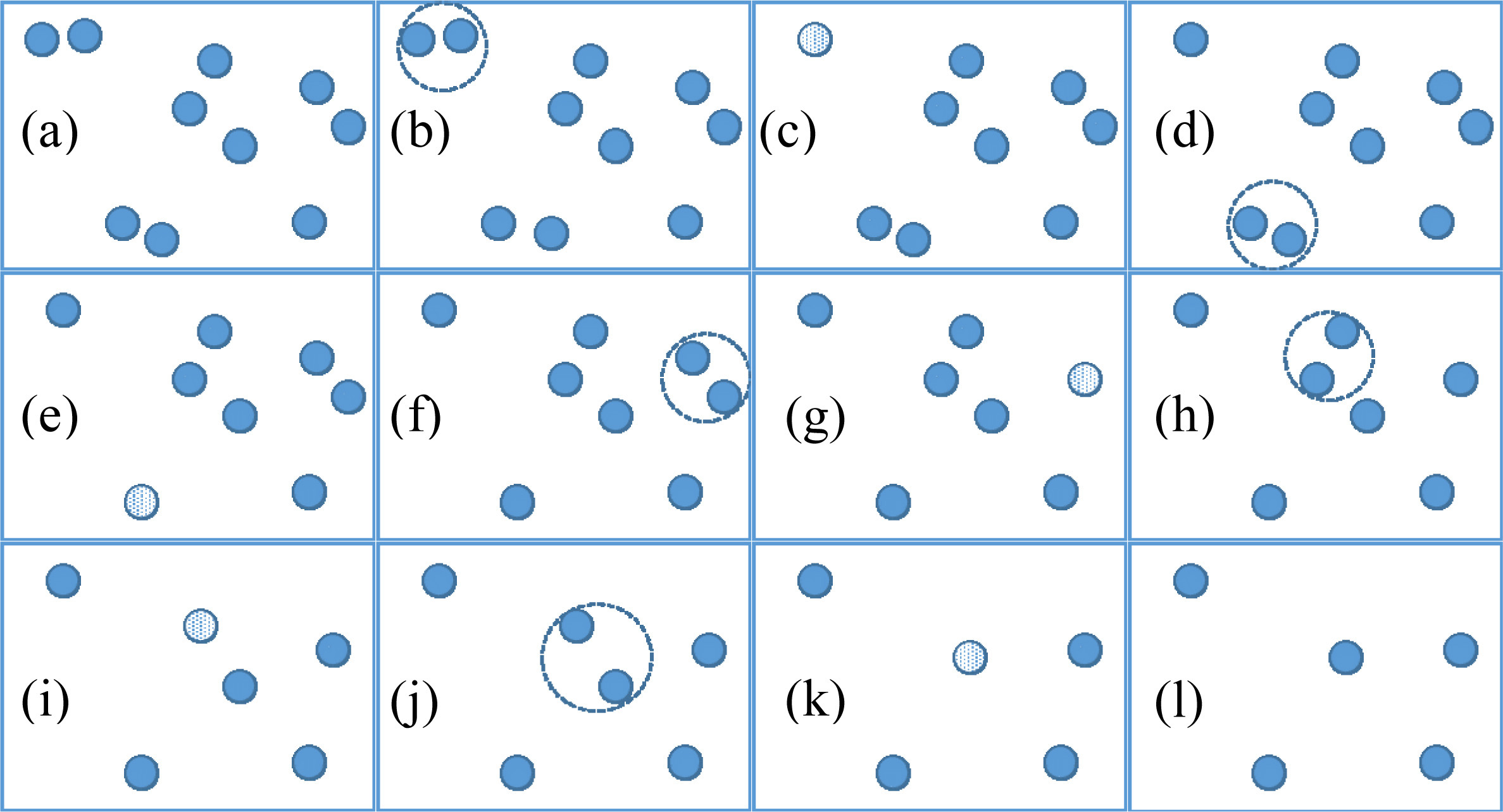

Figure 4 gives an outline of the IR_M algorithm. First the algorithm removes the unrepresentative instances from the training set (line 1). Then, it tries to find a pair of most similar instances in the training set in order to combine them into one instance. So, after each iteration, the number of instances in the training set decreases by one (line 3). There are two different ways to stop the iterative process in the IR_M algorithm. The algorithm repeats until it reaches to the required number of kept instances given by user, for example, 10%, 50%, or 60% of the total number of instances in the training set (Fig. 4) or the algorithm repeats until it can not find any pair of instances in the training set to combine (Fig. 5). So the IR_M algorithm can be used as parameter-free (Fig. 5) or with parameter (Fig. 4). This choice depends on whether the user really wants to control the number of kept instances in the training set or not. In some situations, the user has to work under some critical constraints on the available memory space or computational time. In that case, the parameter $p$ may be given based on the maximum space or time the user has for a particular classification problem.

Figure 4.

The IR_M algorithm with the parameter $p$ .

Figure 5.

The IR_M algorithm without parameter $p$ .

4.3.1 Combining the two instances

In the line 5 of the IR_M algorithm in Fig. 4, we need to combine two time series into one time series. We propose two different strategies to do this combination.

Strategy 1: Hybridization

In this strategy, we mix the two time series into one time series. A simple way to do this is to calculate an average time series $B$ of $Q$ and $C$ , i.e. each value $b_{i}$ in time series $B$ can be computed as follows:

$b_{i}=(q_{i}+c_{i})/2$

where $q_{i}$ , $c_{i}$ are the values in time series $Q$ , $C$ respectively.

Strategy 2: Keep one time series and remove the other

In this strategy, we use the other instances in the training set to decide which one in the pair $Q$ and $C$ should be kept and which is removed from the training set. We choose the time series using the following score function:

$\textit{score}\_1st(T)=\sum\limits_{\forall X_{i}\neq T\,{\rm AND}\,\textit{% label}(X_{i})=\textit{label}(T)\,{\rm AND}\,\textit{SIM}(T,X_{i})=\textit{true% }}1$ (6)

The time series with a lower score is removed and the other one is kept in the training set. The rationale of Eq. 6 is that we would select the instances with higher contribution to the accurate classification of the other instances in the training set, i.e. for each time series $X_{i}$ in the training set and $X_{i}$ has the same class with time series $T$ , if $X_{i}$ is also similar to $T$ according to Eq. 5 in Section 4.2, then we add 1 to the score for $T$ . However, when using Eq. 6, the two instances may have the same score. Then, we use a secondary scoring function as follows:

$\textit{score}\_2nd(T)=\sum\limits_{\forall X_{i}\neq T\,{\rm AND}\,\textit{% label}(X_{i})=\textit{label}(T)}{-\textit{CR}(T,X_{i})}$ (7)

where CR is the compression rate as described in Section 4.2. We can see that score_2nd is always less than or equal to zero. The idea behind this formula is that it selects the instance with lower compression rate because this instance is more similar to the other instances. A rare but probable situation is that the two time series also have the same score_2nd. If this situation happens, then we randomly select one of them and remove the other from the training set.

The first strategy is similar in spirit to a Prototype Abstraction algorithm which generates new instance representatives by summarizing on similar training instances [30]. The second strategy is similar in spirit to a Prototype Selection algorithm which selects some training instances and uses them as representatives. Both Prototype Abstraction and Prototype Selection are commonly-used in instance reduction for nearest neighbor classification of conventional data. Our experiments revealed that both strategies used in the IR_M algorithm provide the same time series classification performance.

4.4 OSP: Optimal selection percentage on the training set

There is one question that the previous works have not tackled: how to determine a minimum percentage of the training set at which we should stop removing instances from it. Notice that while reducing the number of instances in the training set, the error rate of the classifier would increase. As our observation, there exists a special point at which the error rate begins to increase significantly. We call this point the Optimal Selection Percentage (OSP). This means that we should not reduce the number of instances in the training set to the point lower than the OSP point.

Figure 6.

The ideal OSP point in 50 Words training set (a), and Swedish Leaf training set (b).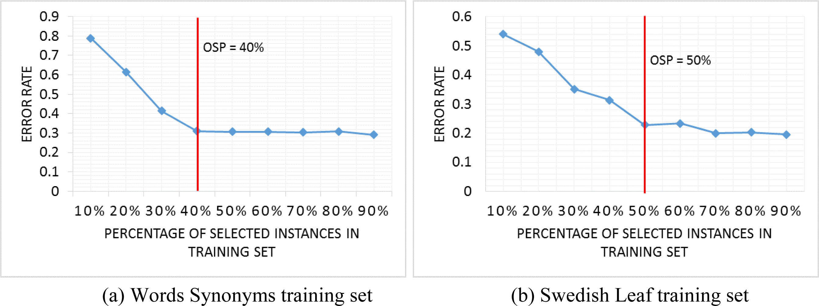

For example, in Fig. 6, we show the error rate over a range of the percentage of selected instances in the training set on two datasets: 50 Words and Swedish Leaf. These datasets also come from the UCR Time Series Classification Archive [8]. As we can see from Fig. 6, in Words Synonyms dataset, the error rate does not change much when we reduce the training set to the point greater than or equal to 40%. But when the training set is reduced to the point lower than 40% of the original training set, the error rate begins to rise significantly. This means that 40% is the point where we should stop removing any more instances. The same situation takes place on Swedish Leaf dataset, 50% is the point where we should stop removing instances from the training set.

In this work, we choose the OSP as the point at which we cannot find any pair of instances in the current training set which are similar, i.e. the compression rate of the two closest instances in the training set becomes greater than 1. This means that whenever the time series $Q$ , and $C$ on line 4 of Fig. 7 satisfy the condition SIM( $Q$ , $C)=$ false, we should stop the instance reduction process. In Fig. 7, we describe a modified version of IR_M algorithm which includes the task of finding the OSP point. Note that the IR_M algorithm in Fig. 7 can be modified in order to accept the percentage parameter $p$ specified by the user.

Figure 7.

The IR_M algorithm with OSP.

4.5 Computational complexity

In our implementation of the RemoveUnrepresentativeInstances algorithm in Fig. 2, first we compute a matrix of size $n\times n$ which stores all the distances from each instance to all the other instances, which computational complexity is $O(n^{2})$ . In step 3, the computational complexity to find the nearest neighbor is $O(n)$ . Because the number of unrepresentative instances usually is not large in comparison to the total number of instances in the training set, we can ignore the complexity of the step removing them from training set (from line 8 to line 11). Therefore, the overall complexity of RemoveUnrepresentativeInstances is $O(n^{2})$ .

In the IR_M algorithm in Fig. 7, first it performs the RemoveUnrepresentativeInstances algorithm. Then, we compute the distances from each instance to all the other instances in the same class and store them in a min-heap. For each iteration, the number of instances in the training set decreases by one, and the operation to find two closest instances of the same class (line 3) is also the operation of removing the smallest element from the min-heap, which complexity is $O(\log(n))$ . Therefore, the overall complexity of IR_M is $O(n^{2})$ , which is equivalent to the complexity of Naïve Rank Reduction and INSIGHT.

5. Experimental evaluation

We implemented our IR_M algorithm and the two previous methods Naïve Rank Reduction, and INSIGHT with Matlab 2012 and conducted the experiments on the Intel Core i7-740QM 1.73 GHz, 4 GB RAM PC. In the experiments, we compare the error rates of our method with those of Naïve Rank Reduction, and INSIGHT method in time series classification. We use each method to reduce the number of instances in the training set. Then, we test the reduced training set by using it to classify the unknown instances in the testing set. We compare the three methods via their error rates. The error rate is the ratio of the correctly classified instances on test data to the total number of tested instances. In general, the lower the error rate is, the better the method is.

5.1 Datasets

Our experiments were conducted over the datasets from the UCR Time Series Classification Archive [8]. There are 44 datasets used in these experiments. These datasets has been downloaded before summer 2015. Each dataset includes a training set and a testing set, and has about 2 to 50 classes. The length of each time series in each datasets is from 60 to 1882. Due to space limit, we do not show details of all the datasets. Interested reader can find more details about these datasets in [8]. Moreover, some details about datasets are also shown when we report the details of some experimental results in Tables 2 and 3 (of Appendix A). Table 2 shows the error rates of 1-Nearest Neighbor Classifier before removing unrepresentative instances (UI) and after removing unrepresentative instances on some datasets. Table 3 shows OSPs and error rates at the OSP point on 44 datasets by IR_M with two different strategies of combining instances.

5.2 Input parameters

For the convenience of comparison to the two previous methods, Naïve Rank Reduction and INSIGHT method, we set Sakoe-Chiba band $r$ of DTW distance to 10% of the time series length. As for cardinality of the MDL principle (described in Section 2.5), through our extensive experiments, we decide to reduce time series data to its 8-value (3-bit) cardinality version.

5.3 Overall experimental results on the 44 datasets

In this subsection, we report the overall comparison of IR_M with Naïve Rank Reduction and INSIGHT. For each datasets from 44 datasets [8], we apply the three methods on them; then, we test the output training set by applying 1-Nearest Neighbor Classifier on the testing part of the dataset. We record the error rates of the three methods on each dataset and compare them. The method with lower error rate is marked as winner. Figure 8 shows two area charts of the overall comparison of IR_M with the two pervious methods over the datasets.

In Fig. 8(a), we show the comparison of IR_M to Naïve Rank Reduction. As we can see from the area chart, IR_M outperforms Naïve Rank Reduction when we keep the number of selected instances greater than or equal to 40% of the original training set. At these percentages, on nearly two thirds of the training sets, IR_M method performs better than or equal to the pervious method. For example, when the number of selected instances is equal to 50% of the size of the training set, IR_M wins in 29 datasets, draws in 4 datasets and loses in 11 datasets. When the number of selected instances is equal to 75% of the size of the training set, IR_M wins in 32 datasets, draws in 6 datasets and loses in 6 datasets. When the number of selected instances is lower than 40%, Naïve Rank Reduction tends to performs better. For example, when the number of selected instances is equal to 10%, IR_M wins in 16 datasets, whereas Naïve Rank Reduction wins in 27 datasets, and they draw in 1 dataset.

Figure 8.

Comparing the error rates of IR_M to Naïve Rank Reduction, and INSIGHT over the 44 datasets.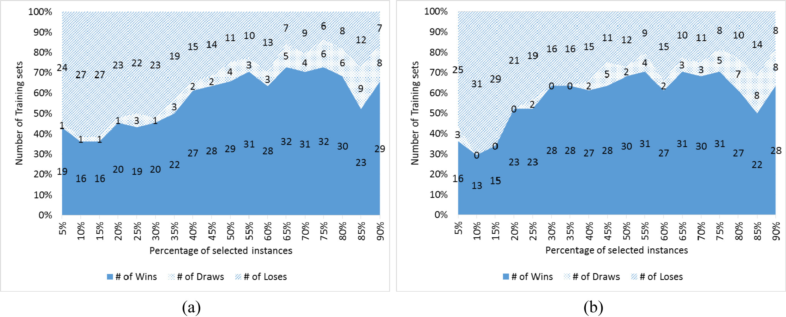

Figure 8(b) shows the comparison of IR_M to INSIGHT method. In general, IR_M outperforms INSIGHT when we keep the number of instances in the training set greater than or equal to 30% of the original training set. At these percentages, nearly two thirds of the training sets, IR_M method performs better or equal to the previous one. For example, at the reduction of 50%, IR_M performs better than INSIGHT in 30 datasets, draws in 2 datasets and loses in 12 datasets. When the number of selected instances is equal to 75% of the size of the training set, IR_M wins in 31 datasets, draws in 5 datasets and loses in 8 datasets. When the number of selected instances is lower than 30%, INSIGHT method performs better. For example, when the number of selected instances is equal to 10%, IR_M wins in 13 datasets, and INSIGHT wins in 31 datasets.

In the next subsection, we will show the details of the comparative experimental results on some datasets.

5.4 Details of comparative experimental results on some datasets

5.4.1 OSU leaf dataset

There are 6 classes in this dataset which includes two separate subsets: the training set and the testing set. The training set contains 200 time series and the testing set contains 242 time series. Each time series consists of 427 data points. Figure 9 shows the comparison of IR_M to the two previous methods Naïve Rank Reduction and INSIGHT. When the percentage of selected instances in the training set is greater than 50%, the error rate of IR_M method is lower than the Naïve Rank Reduction and INSIGHT; meanwhile, when the percentage is lower than 50%, they are nearly the same.

Figure 9.

A comparison of IR_M to Naïve Rank and INSIGHT in OSU Leaf dataset when the reduction is greater than 50% instances (a) and lower than 50% instances (b).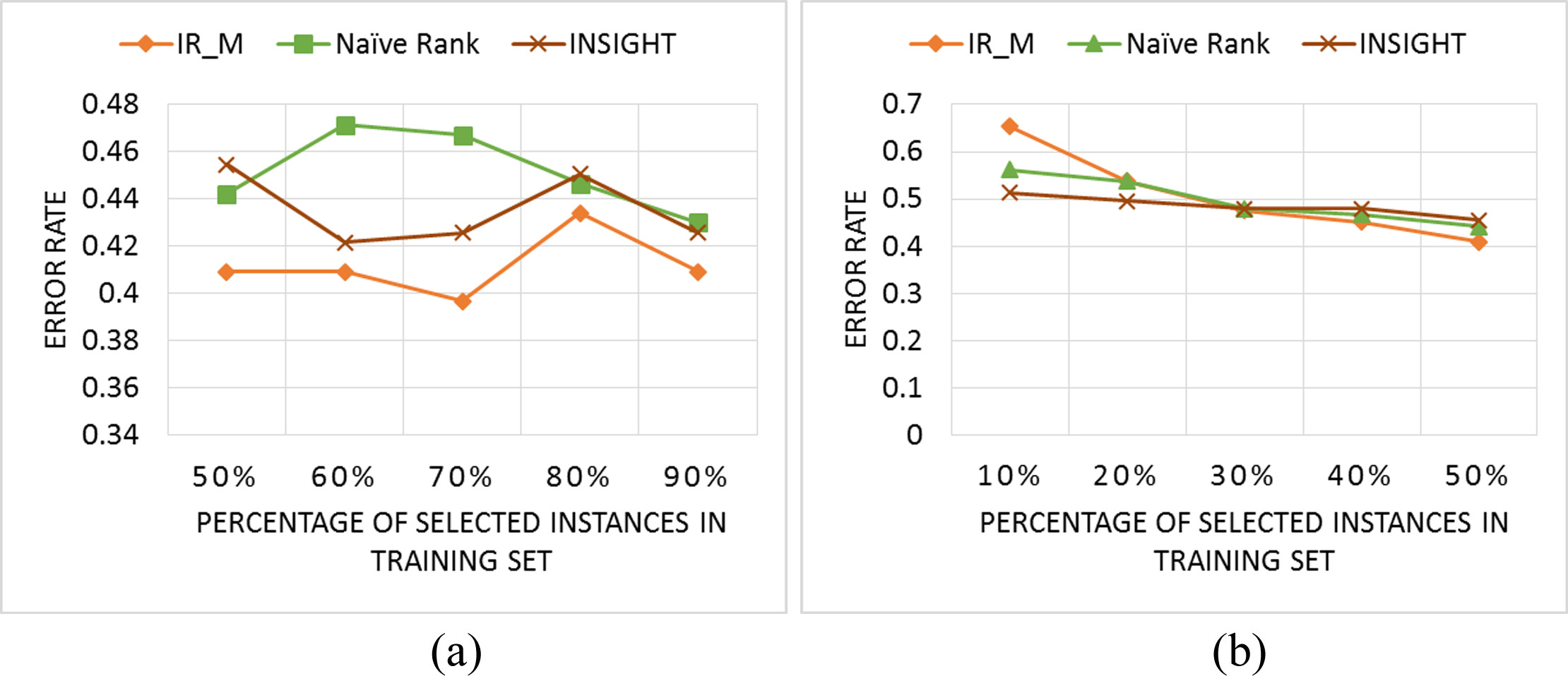

5.4.2 Medical images dataset

There are 10 classes in this dataset which includes two separate subsets: the training set and the testing set. The training set contains 381 time series and the testing set contains 760 time series. Each time series consists of 99 data points. Figure 10 shows the comparison of IR_M to the two previous methods Naïve Rank Reduction and INSIGHT. When the percentage of selected instances in the training set is greater than 30%, the error rates of IR_M are nearly the same, and they are both better than those of the Naïve Rank Reduction and INSIGHT method; meanwhile, when the percentage is lower than 30%, the INSIGHT seems to be the best method, next is IR_M, and Naïve Rank Reduction is the worst in this case.

Figure 10.

A comparison of IR_M to Naïve Rank and INSIGHT in Medical Images dataset when the reduction is greater than 30% instances (a) and lower than 30% instances (b).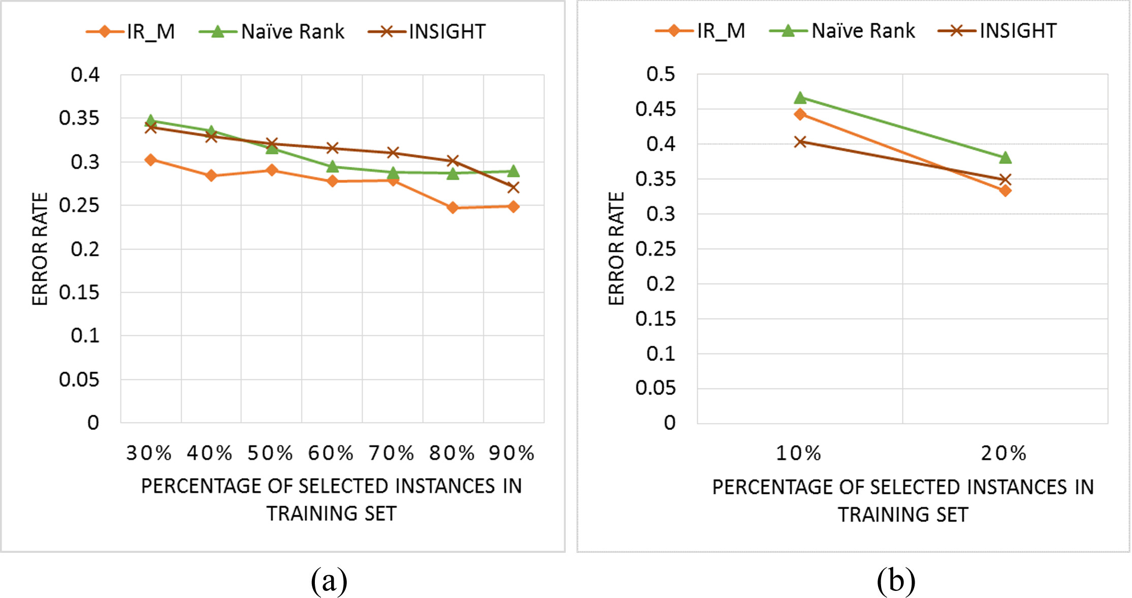

5.4.3 Gun point dataset

There are 2 classes in this dataset which includes two separate subsets: the training set and the testing set. The training set contains 50 time series and the testing set contains 150 time series. Each time series consists of 150 data points. Figure 11 shows the comparison of IR_M to the two previous methods Naïve Rank Reduction and INSIGHT. When the percentage of selected instances in the training set is greater than 50%, the error rate of IR_M method is lower than that of the Naïve Rank Reduction and INSIGHT; meanwhile, when the percentage is lower than 50%, the two pervious methods and IR_M are nearly the same, and when the percentage is lower than 30%, the IR_M is worse than the two previous methods.

Figure 11.

A comparison of IR_M and Naïve Rank and INSIGHT in Gun Point dataset of selected greater than 50% instances (a) and lower than 50% instances (b).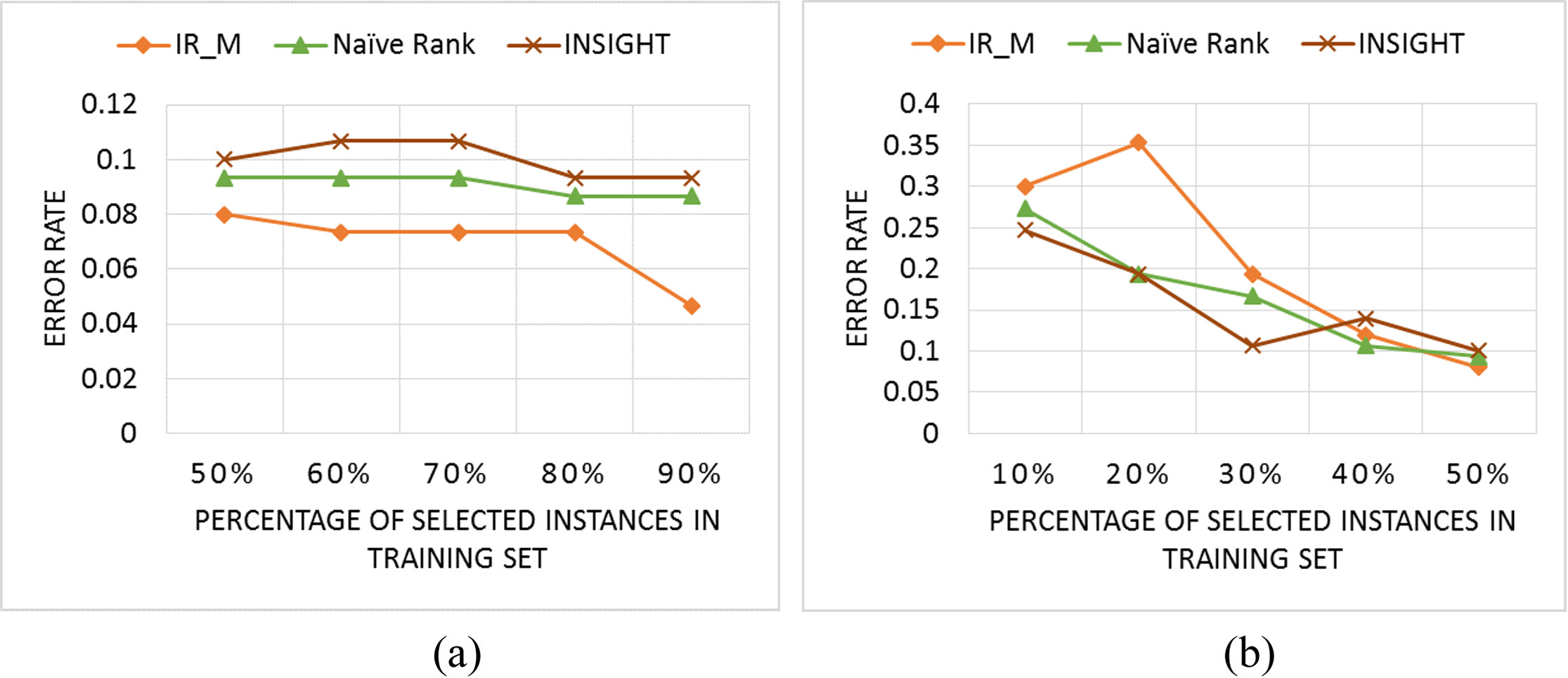

5.4.4 Face four dataset

There are 4 classes in this dataset which includes two separate subsets: the training set and the testing set. The training set contains 24 time series and the testing set contains 88 time series. Each time series consists of 350 data points. Figure 12 shows the comparison of IR_M to two previous methods Naïve Rank Reduction and INSIGHT. As we can see from the figures, the error rate of IR_M method is lower than that of the Naïve Rank Reduction and INSIGHT.

Figure 12.

A comparison of IR_M and Naïve Rank and INSIGHT in Face Four dataset with the reduction varying from 10% to 30%.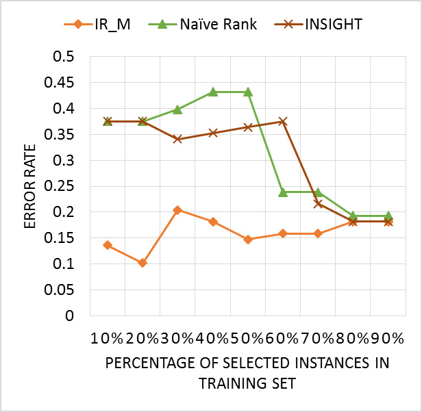

5.4.5 CBF dataset

There are 3 classes in this dataset which includes two separate subsets: the training set and the testing set. The training set contains 30 time series and the testing set contains 900 time series. Each time series consists of 128 data points. Figure 13 shows the comparison of IR_M to the two previous methods Naïve Rank Reduction and INSIGHT. When the percentage of selected instances in the training set is greater than 30%, the error rate of IR_M method is lower than that of the Naïve Rank Reduction and INSIGHT; meanwhile, when the percentage is lower than 30%, IR_M and INSIGHT are nearly the same, and next is Naïve Rank Reduction.

Figure 13.

A comparison of IR_M and Naïve Rank and INSIGHT in CBF dataset when the reduction is greater than 30% instances (a) and lower than 30% instances (b).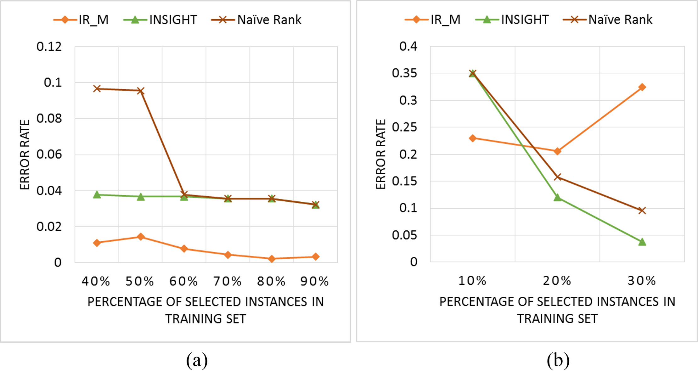

5.5 Experiment on choosing the OSP

In the above experiments, we show that IR_M tends to be better than Naïve Rank Reduction and INSIGHT when the percentage of selected instances in the training set is about greater than 30%. This is not always true, but most of the datasets seem satisfying this rule. Now we would like to give some discussion on this observation.

The main idea behind the Naïve Rank Reduction and INSIGHT is to use statistics to decide “How good is an instance?” by measuring the contribution of that instance to classification of local training set, i.e. they use other instances in the training set to measure the impact of one instance in this training set. And this impact is supposed to be the same outside the training set.

Figure 14.

OSP of Words Synonyms dataset of IR_M by strategy 1 (a) and strategy 2 (b).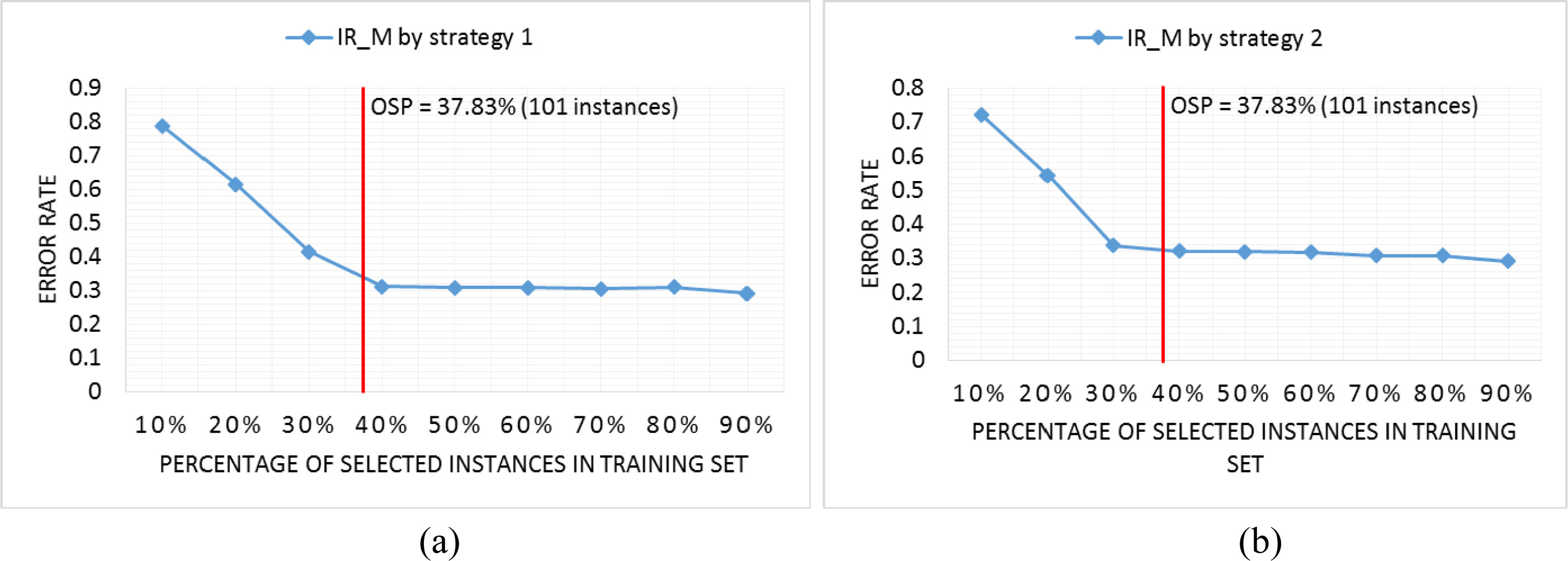

Our method IR_M is based on another perspective. We consider the whole training set as a data set, and we attempts to compress it as much as we can. To achieve this goal, at each iteration, we combine two instances with the same features into one instance. Thank to that, we can keep the best representative instances in the training set. However, when the training set has been reduced to some limit that we cannot find any pair of instances with the same features; if we continue to combine the instances, we will lose some of the representative instances. That is why when IR_M goes beyond some limit of the number of kept instances; it performs worse than the two pervious methods.

Figure 15.

OSP of 50 Words dataset of IR_M by strategy 1 (a) and strategy 2 (b).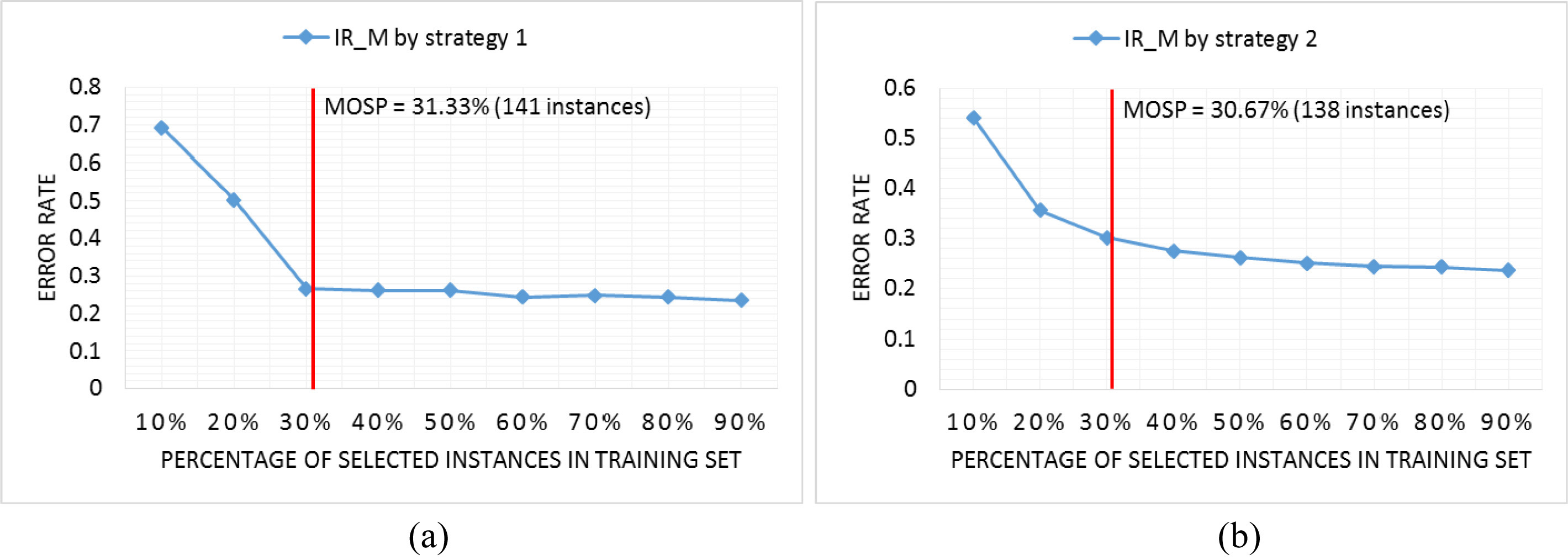

Now, we report some experiments on finding the OSP. Notice that the method of selecting OSP in our instance reduction algorithm is just a heuristic.

Figure 14 shows the OSP on Words Synonyms dataset. With this dataset, the OSP determined by IR_M is about 37.83%.

Figure 15 shows the OSP on 50 Words dataset. With this dataset, the OSP given by IR_M is about 31.33%. As we can see from Figs 14 and 15, the OSPs found on these datasets are the robust stopping points.

In addition, more experimental results about OSPs on the other datasets are re-ported in Table 3 (of Appendix A).

5.6 Experiment on time efficiency

Table 1 reports the execution times (in seconds) needed to perform instance reduction with our IR_M, Naïve Rank Reduction and INSIGHT over 44 datasets. As expected, our method performs with the same time efficiency as those of the two previous methods. Among 44 datasets, for some datasets, our method runs faster than Naïve Rank Redution or INSIGHT, but for some other datasets, our method runs slower than Naïve Rank Redution or INSIGHT.

Table 1
Running times (seconds) of 4 algorithms on 44 datasets

Datasets	IR_M_STR1	IR_M_STR2	Naïve Rank	INSIGHT
50words	37.1702	41.1334	35.6919	44.5414
Adiac	12.9238	14.2368	17.9938	16.6403
Beef	0.11035	0.097414	0.14297	0.11544
CBF	0.29435	0.27388	0.2353	0.25948
ChlorineConcentration	22.15	14.6017	7.683	5.2384
CinC_ECG_torso	4.1557	4.2447	5.5913	4.3602
Coffee	0.44298	0.25022	0.23763	0.20324
Cricket_X	37.8989	42.2277	42.411	36.1098
Cricket_Y	82.3843	86.5713	79.0802	79.591
Cricket_Z	40.3372	40.4448	38.5028	36.472
DiatomSizeReduction	0.057096	0.036897	0.022749	0.020012
ECG200	1.9361	1.3196	0.33719	0.24753
ECGFiveDays	0.096122	0.066613	0.02634	0.022956
FaceAll	33.0813	27.6354	23.6239	20.8529
FaceFour	0.24529	0.24064	0.27894	0.24688
FacesUCR	9.1319	9.5861	10.6854	9.9663
FISH	15.6121	18.4934	16.1181	16.078
Gun_Point	0.54161	0.37495	0.13302	0.099203
Haptics	46.7264	43.4048	43.4887	42.5788

5.7 Discussion of the MDL choice

Now that the reader has gleaned some intuition of our instance reduction method for time series; we will briefly revisit a discussion of why MDL principle is our choice in this work.

We can use any distance function such as Euclidean Distance, Dynamic Time Warping or Complexity Invariant Distance [2], etc. to calculate the similarity between two time series. The distance between two time series is then compared with a pre-specified threshold $r$ . If the distance between two time series is lower than or equal to the threshold $r$ , they are considered similar; otherwise, they are considered different. This approach is usually called Range Search problem. However, this approach has a drawback since it requires us providing a threshold to distinguish similar instances and different instances in a set of time series. This threshold always depends highly on the characteristics of the data in the underlying application and hence it is not trivial to estimate this threshold. On the contrary, when using MDL principle, our method can automatically determine whether two time series are similar or not without requiring any threshold parameter by using the compression rate between two time series (as described in Section 4.2). In other words, we choose MDL principle because we want to take advantage of its intrinsically parameter-free nature which helps us not to use any domain-knowledge in our proposed instance reduction method for time series classification.

6. Conclusions and future works

In this paper, we propose a new MDL-based method, called IR_M, to reduce the number of instances in the training set for time series classification. In our method we regard the whole training set as a data set and attempt to compress it as much as we can. That means at each iteration in our IR_M algorithm if we can compress the two time series by the MDL principle, we combine them into one time series. To our knowledge, this is the first work addressing instance reduction for time series classification using MDL principle. Experimental results show that our method can outperform INSIGHT and Naïve Rank Reduction when the number of selected instances in the training set is not too small.

As for future work, we intend to apply some other distance measures for our instance reduction method such as Complexity-Invariant Distance [2] or Compression Rate Distance [33] because distance measure has a huge impact on time series classification problem. We also plan to combine our method with some features of the two previous methods INSIGHT and Naïve Rank Reduction since they can work together better with a very small number of kept instances in the training set.

Footnotes

Acknowledgments

We would like to thank Prof. Eamonn Keogh for kindly sharing the datasets which help us in constructing the experiments in this work.

Appendix A: More experimental results

Table 2

The error rate of 1-nearest neighbor classifier before removing unrepresentative instances (UI) and after removing unrepresentative instances on some datasets

Datasets	Size of original	Number	Size of removed	Error rate before	Error rate after
	training set	of UI	UI training set	remove UI	remove UI
50words	450	74	376	0.23956	0.24396
Beef	30	13	17	0.5	0.56667
ECG200	100	12	88	0.18	0.15
FaceAll	560	16	544	0.20947	0.21953
FISH	175	32	143	0.16	0.17143
Gun_Point	50	1	49	0.06	0.053333
Haptics	155	69	86	0.60065	0.57792
Lighting2	60	6	54	0.098361	0.16393
Lighting7	70	12	58	0.26027	0.23288
MoteStrain	20	3	17	0.13738	0.11502
OSULeaf	200	43	157	0.39669	0.43388
MedicalImages	381	98	283	0.25526	0.27895
WordsSynonyms	267	53	214	0.27273	0.30878

Table 3

OSP and error rate at the OSP point on 44 datasets

Datasets	Size of	IR_M_STR1			IR_M_STR2
	original	Number of	OSP	Error	Number of	OSP	Error
	training set	selected instances		rate	selected instances		rate
50words	450	141	31.33	0.27033	138	30.67	0.2967
Adiac	390	37	9.49	0.61637	37	9.49	0.60102
Beef	30	6	20	0.56667	7	23.33	0.56667
CBF	30	11	36.67	0.20667	13	43.33	0.013333
Chlorine ${}^{1}$	467	7	1.5	0.70573	9	1.93	0.59974
CinC_ECG ${}^{2}$	40	28	70	0.36957	28	70	0.36884
Coffee	28	2	7.14	0.32143	2	7.14	0.46429
Cricket_X	390	167	42.82	0.29744	165	42.31	0.24615
Cricket_Y	390	150	38.46	0.30513	156	40	0.25385
Cricket_Z	390	164	42.05	0.27949	169	43.33	0.24103
Diatom ${}^{3}$	16	4	25	0.21895	4	25	0.12418
ECG200	100	5	5	0.61	4	4	0.29
ECGFiveDays	23	10	43.48	0.34727	12	52.17	0.36121
FaceAll	560	116	20.71	0.18698	126	22.5	0.34142
FaceFour	24	7	29.17	0.14773	7	29.17	0.28409
FacesUCR	200	72	36	0.17707	78	39	0.21805
FISH	175	7	4	0.61714	7	4	0.49143
Gun_Point	50	6	12	0.3	6	12	0.3
Haptics	155	12	7.74	0.73377	14	9.03	0.69481
InlineSkate	100	16	16	0.73273	14	14	0.75636
ItalyPower ${}^{4}$	67	3	4.48	0.10982	3	4.48	0.40622
Lighting2	60	36	60	0.21311	37	61.67	0.18033
Lighting7	70	36	51.43	0.31507	42	60	0.21918
MALLAT	55	8	14.55	0.089552	8	14.55	0.14371
MedicalImages	381	57	14.96	0.39079	61	16.01	0.38289
MoteStrain	20	8	40	0.19728	8	40	0.1885
OliveOil	30	4	13.33	0.13333	4	13.33	0.6
OSULeaf	200	46	23	0.52893	48	24	0.47107
SonyII ${}^{5}$	27	8	29.63	0.18888	7	25.93	0.20147
Sony ${}^{6}$	20	3	15	0.32113	3	15	0.34775
SwedishLeaf	500	27	5.4	0.6064	22	4.4	0.4272
Symbols	25	8	32	0.11859	8	32	0.078392
synthetic_control	300	69	23	0.076667	67	22.33	0.063333
Trace	100	8	8	0.1	7	7	0.15
TwoLeadECG	23	2	8.7	0.30378	3	13.04	0.3626
Two_Patterns	1000	460	46	0.00075	443	44.3	0.0005
uWave_X ${}^{7}$	896	84	9.38	0.37912	84	9.38	0.38079
uWave_Y ${}^{8}$	896	65	7.25	0.3981	51	5.69	0.46036
uWave_Z ${}^{9}$	896	66	7.37	0.42518	68	7.59	0.41374
wafer	1000	42	4.2	0.10788	43	4.3	0.062622
WordsSynonyms	267	101	37.83	0.31661	101	37.83	0.32288
yoga	300	11	3.67	0.41367	10	3.33	0.45767
Thorax1 ${}^{11}$	1800	45	2.5	0.51654	43	2.39	0.52316
Thorax2 ${}^{12}$	1800	45	2.5	0.40509	43	2.39	0.41578

Note that some dataset names in Table 2 and Table 3 are originally as follows: ${}^{1}$ ChlorineConcentration, ${}^{2}$ CinC_ECG_torso,

${}^{3}$ DiatomSizeReduction, ${}^{4}$ ItalyPowerDemand, ${}^{5}$ SonyAIBORobotSurfaceII, ${}^{6}$ SonyAIBORobotSurface,

${}^{7}$ uWaveGestureLibrary_X, ${}^{8}$ uWaveGestureLibrary_Y, ${}^{9}$ uWaveGestureLibrary_Z, ${}^{10}$ uWaveGestureLibrary_Z,

${}^{11}$ NonInvasiveFatalECG_Thorax1, ${}^{12}$ NonInvasiveFatalECG_Thorax2.

References

Assent

Krieger

Afschari

and Seidl

, The TS-tree: Efficient time series search and retrieval, in: Proceedings of the 11th International Conference on Extending Database Technology: Advances in Database Technology (EDBT ’08), (2008), 252–263.

Batista

Keogh

Tataw

O.M.

and Souza

V.M.A.D.

, CID: An efficient complexity-invariant distance for time series, Data Mining and Knowledge Discovery 8 (2014), 634–669.

Beckmann

Kriegel

H.-P.

Schneider

and Seeger

, The R*-tree: An efficient and robust access method for points and rectangles, ACM SIGMOD Record SIGMOD Rec, (1990), 322–331.

Begum

Rakthanmanon

and Keogh

, A minimum description length technique for semi-supervised time series classification, in: Integration of Reusable Systems Advances in Intelligent Systems and Computing, (2014), 171–192.

Bemdt

D.J.

and Clifford

, Using dynamic time warping to find patterns in time series, in: Proceedings of AAAI Workshop on Knowledge Discovery in Databases, Seattle, Washington, USA, (1994), 359–370.

Brighton

and Mellish

, Advances in instance selection for instance-based learning algorithms, Data Mining and Knowledge Discovery 6 (2002), 153–172.

Buza

Nanopoulos

and Schmidt-Thieme

, INSIGHT: Efficient and effective instance selection for time-series classification, in: Proc of 15th Pacific-Asia Conference on Knowledge Discovery and Data Mining (PAKDD 2011), Shenzhen, China, May 24–27, Part II, (2011), 149–160.

Chen

Keogh

Begum

Bagnall

Mueen

and Batista

, The UCR time series classification archive, URL www.cs.ucr.edu/∼eamonn/time_series_data/, 2015.

Ciaccia

Patella

and Zezula

, M-tree: An efficient access method for similarity search in metric spaces, in: VLDB ’97 Proceedings of the 23rd International Conference on Very Large Data Bases, (1997), 426–435.

10.

Garcia

Derrac

Cano

J.R.

and Herrera

, Prototype selection for nearest neighbor classification: Taxonomy and empirical study, IEEE Trans on Pattern Analysis and Machine Intelligence 34(3) (2012), 417–435.

11.

Grünwald

P.D.

, The minimum description length principle, MIT Press, Cambridge, Mass, 2007.

12.

Guttman

, R-trees: A dynamic index structure for spatial searching, in: SIGMOD ’84 Proceedings of ACM SIGMOD International Conference on Management of Data, (1984), 47–57.

13.

and Deng

, Discovering cluster-based local outliers, Pattern Recognition Letters 24 (2003), 1641–1650.

14.

Rakthanmanon

Hao

Evans

Lonardi

and Keogh

, Discovering the intrinsic cardinality and dimensionality of time series using MDL, Proc of ICDM, (2011).

15.

Itakura

, Minimum prediction residual principle applied to speech recognition, IEEE Transactions on Acoustics, Speech, and Signal Processing IEEE Trans Acoust, Speech, Signal Process ASSP-23 (1975), 67–72.

16.

Jankowski

and Grochowski

, Comparison of instance selection algorithms I, algorithms survey, in: ICAISC, LNCS 3070, Springer, (2004), 598–603.

17.

Jankowski

and Grochowski

, Comparison of instance selection algorithms II, results and comments, in: ICAISC, LNCS 3070, Springer, (2004), 580–585.

18.

Jiang

M.F.

Tseng

S.S.

and Su

C.M.

, Two-phase clustering process for outliers detection, Pattern Recognition Letters 22 (2001), 691–700.

19.

Keogh

Chakrabarti

Pazzani

and Mehrotra

, Dimensionality reduction for fast similarity search in large time series databases, Knowledge and Information Systems 3 (2001), 263–286.

20.

Keogh

and Pazzani

, An enhanced representation of time series which allows fast and accurate classification, clustering and relevance feedback, in: Proceedings of the 4th International Conference on Knowledge Discovery and Data Mining, (1998), 239–241.

21.

Keogh

and Ratanamahatana

C.A.

, Exact indexing of dynamic time warping, Knowledge and Information Systems 7 (2005), 358–386.

22.

Kim

S.W.

and Park

, An index-based approach for similarity search supporting time warping in large sequence databases, Proceedings of the 17th IEEE International Conference on Data Engineering, Heidelberg, Germany, (2001), 607–614.

23.

Lemire

, Faster retrieval with a two-pass dynamic-time-warping lower bound, Pattern Recognition 42(9) (2009), 2169–2180.

24.

Lin

Keogh

Lonardi

and Chiu

, A symbolic representation of time series, with implications for streaming algorithms, in: Proceedings of the 8th ACM SIGMOD Workshop on Research Issues in Data Mining and Knowledge Discovery (DMKD ’03), (2003), 2–11.

25.

Radovanovic

Nanopoulos

and Ivanovic

, Nearest neighbor in high-dimensional data: The emergence and influence of hubs, ICML’09 (2009).

26.

Rakthanmanon

Campana

Mueen

Batista

Westover

Zhu

Zakaria

and Keogh

, Searching and mining trillions of time series subsequences under dynamic time warping, in: Proceedings of the 18th ACM SIGKDD International Conference on Knowledge Discovery and Data Mining (KDD ’12), (2012), 262–270.

27.

Rakthanmanon

Keogh

Lonardi

and Evans

, MDL-based time series clustering, Knowledge and Information Systems 33 (2012), 371–399.

28.

Rissanen

, Modeling by shortest data description, Automatica 14 (1978), 465–471.

29.

Sakoe

and Chiba

, Dynamic programming algorithm optimization for spoken word recognition, in: IEEE Transactions on Acoustics, Speech, and Signal Processing IEEE Trans Acoust, Speech, Signal Process ASSP-26 (1978), 43–49.

30.

Shokoohi-Yekta

Chen

Campana

Zakaria

and Keogh

, Discovery of meaningful rules in time series, in: Proc of SIGKDD, (2015).

31.

Tanaka

Iwamoto

and Uehara

, Discovery of time-series motif from multi-dimensional data based on MDL principle, Machine Learning 58 (2005), 269–300.

32.

Triguero

Derrac

Garcia

and Herrera

, A Taxonomy and experimental study on prototype generation for nearest neighbor classification, IEEE Trans on Systems, Man, and Cybernetics-Part C: Applications and Reviews 41(1) (2012), 86–100.

33.

Vinh

V.T.

and Anh

D.T.

, Compression rate distance measure for time series, in: Proceedings of 2015 IEEE International Conference on Data Science and Advanced Analytics (DSAA 2015), IEEE, Paris, France, October 19–24, (2015), 1–10.

34.

Wang

Mueen

Ding

Trajcevski

Scheuermann

and Keogh

, Experimental comparison of representation methods and distance measures for time series data, Data Mining and Knowledge Discovery 26 (2013), 275–309.

35.

Wilson

D.L.

, Asymptotic properties of nearest neighbor rules using edited data, IEEE Transactions on Systems, Man, and Cybernetics 2(3) (1972), 408–421.

36.

Wilson

D.R.

and Martinez

T.R.

, Instance pruning techniques, in: Proc of ICML’97, Morgan Kaufmann, (1997), 403–411.

37.

Wilson

D.R.

and Martinez

T.R.

, Reduction techniques for instance-based learning algorithms, Machine Learning 38 (2000), 257–286.

38.

Keogh

Shelton

Wei

and Ratanamahatana

C.A.

, Fast time series classification using numerosity reduction, in: Proceedings of the 23rd International Conference on Machine Learning (ICML ’06), (2006), 1033–1040.

Instance reduction for time series classification using MDL principle

Abstract

Keywords

1. Introduction

2. Backgrounds

2.1 Time series

2.2 1-Nearest Neighbor Classifier

2.3 Distance measures on time series

2.4 Dynamic Time Warping

2.5.1 Discrete normalization function

2.5.2 Entropy

2.5.3 Description length

2.5.4 Hypothesis

2.5.5 Conditional description length

3. Related works

3.1 Naïve Rank Reduction

4. IR_M: Reducing the training set based on MDL principle

4.1 Unrepresentative instances

4.1.1 Definition of unrepresentative instance (UI)

4.1.2 Effects of unrepresentative instances

4.1.3 Removing the unrepresentative instances

4.2 Similar and different instances

Strategy 1: Hybridization

Strategy 2: Keep one time series and remove the other

5. Experimental evaluation

5.1 Datasets

5.2 Input parameters

5.3 Overall experimental results on the 44 datasets

5.4.1 OSU leaf dataset

Table 1 Running times (seconds) of 4 algorithms on 44 datasets

6. Conclusions and future works

Footnotes

Acknowledgments

Appendix A: More experimental results

References

Table 1
Running times (seconds) of 4 algorithms on 44 datasets