Multilevel dynamic time warping: A parameter-light method for fast time series classification

Abstract

Time series classification is a fundamental problem in the time series mining community. Recently, many sophisticated methods which can produce state-of-the-art classification accuracy on the UCR archive have been proposed. Unfortunately, most of them are parameter-laden methods and require fine-tune for different datasets. Besides, training these classifiers is very computationally demanding, which makes them difficult to use in many real-time applications and previously unseen datasets. In this paper, we propose a novel parameter-light algorithm, MDTW, to classify time series. MDTW has a few parameters which do not require any fine-tune and can be chosen arbitrarily because the classification accuracy is largely insensitive to the parameters. MDTW has no training step; thus, it can be directly applied to unseen datasets. MDTW is based on a popular method, namely the nearest neighbor classifier with Dynamic Time Warping (NN-DTW). However, MDTW performs much faster than NN-DTW by representing time series in different resolutions and using filters-and-refine framework to find the nearest neighbor. The experimental results demonstrate that MDTW performs faster than the state-of-the-art, with small losses (<3%) in average classification accuracy. Besides, we embed a technique, prunedDTW, into the MDTW procedure to make MDTW even faster, and show by experiments that this combination can speed up the MDTW from one to five times.

Keywords

Time series classification Dynamic Time Warping nearest neighbor multilevel representations filters-and-refine

1 Introduction

Time series classification (TSC) is one of the most challenging problems and widely used in the time series data mining community. With the growing popularity of temporal data, TSC has been highly applied to many real-world applications, including human activity recognition [44], classification of Electrocardiograms [22], acoustic scene classification [28], speech recognition [38], and many more.

TSC differs from traditional classification problems because time series are always high-dimensional data, and the order of the attributes does matter. In the past few years, a multitude of inspiring algorithms have been investigated to solve the TSC problem, and the greatest research emphasis has been focused on improving the classification accuracy. Representative methods include Elastic Ensemble (EE) [26], Bag-of-SFA-Symbols (BOSS) [35], Shapelet Transform (ST) [16], Collective of Transformation-based Ensembles (COTE) [2], Hierarchical Vote COTE (HIVE-COTE) [27]. These methods are sophisticated and can garner state-of-the-art classification accuracy on the UCR archive [10], which is the primary benchmark for TSC researches. Unfortunately, these newly developed methods suffer from two main drawbacks, which limit their use in many real-life applications.

Firstly, most of the mentioned TSC algorithms require the setting of input parameters, and the researcher is always forced to fine-tune the parameters to achieve the optimal results [14]. Nevertheless, these parameters are dependent on the dataset, and the unsatisfactory results may be obtained if poorly parameter settings are chosen. Thus, these parameter-laden methods can not be directly applied to previously unseen datasets because the trained models rely on a particular dataset [43]. Besides, training these high accuracy classifiers, such as COTE and HIVE-COTE, has very high space and time complexity. For example, training HIVE-COTE on a time series dataset with only 1500 instances can require eight days of CPU time [39]. Therefore, HIVE-COTE is infeasible for many real-life applications, although it can achieve state-of-the-art classification accuracy.

Secondly, in many domains, time series data such as sensor data can be very dynamic. For many parameter-laden methods, it is challenging to generate a trained model when time series in the real-time analytics or mutable database because the user may need to change the model frequently.

We believe that the NN-DTW [42] is an effective TSC method for overcoming these drawbacks. This is for two main reasons: (1) NN-DTW is a non-parametric TSC method that can be directly exploited with mutable and previously unseen datasets. (2) NN-DTW has been widely used and can achieve performance which is not significantly different than the state-of-the-art. However, calculating DTW distance between two time series is rather slow because DTW has quadratic time complexity. Thus, NN-DTW cannot scale well to real-time applications where the responsiveness is essential. With these motivations, in this paper, our objective is to design a parameter-light and efficient method to solve TSC problem. Specifically, the MDTW (shorthand for Multilevel Dynamic Time Warping) is proposed. The MDTW is based on NN-DTW; however, it performs much faster than NN-DTW. The MDTW is a parameter-light method. It involves only a few parameters and needs not to fine-tune the parameters for different datasets. More importantly, the parameters can be chosen arbitrarily because the classification accuracy is largely insensitive to the parameters. MDTW has a pre-processing step; however, the pre-processing time is very small (less than one second) even on large time series datasets, and thus, the overhead of the pre-processing step can be ignored.

To summarize, we make the following contributions

In this paper, we propose the MDTW method for time series classification problem. The MDTW involves several different resolutions for time series representations and uses the filters-and-refine framework to calculate the nearest neighbor. Many expensive DTW distance computations can be reduced in the filters-stage. Thus, MDTW can speed up the conventional NN-DTW procedure.

The MDTW is orthogonal to most of the methods of accelerating DTW computations and can be used in conjunction with them. To illustrate this point, in this paper, we embed a recently presented technique, prunedDTW [40], into the MDTW procedure to make MDTW even faster.

We compare the performance of MDTW with related state-of-the-art methods using the UCR archive. The experimental results show that MDTW achieves similar classification accuracy as NN-DTW. Furthermore, there is no significant difference between our approach and the state-of-the-art in average accuracy, with very small losses (<3%). The empirical studies also demonstrate that MDTW is orders of magnitude faster than the competitors.

The paper is organized as follows. Section 2 presents the necessary background knowledge and related work of our research. In Section 3, we start with some necessary definitions, as well as with a brief introduction of the DTW distance. We then describe the intuition behind our method and give the formal statement and time complexity analysis of the MDTW. The experimental results can be found in Section 4. Finally, the paper is concluded in Section 5.

2 Background

2.1 Time series classification

Given a time series training set, the task of TSC is to train a classifier on a training set and use this classifier to predict the class labels of unlabeled time series. A multitude of techniques have been proposed and we can classify these techniques into five types [1], i.e., interval-based [5 , 12], shapelet-based [7 , 29], dictionary-based [25 , 37], ensemble-based [2, 27] and instance-based [17 , 51].

Interval-based methods. These methods train a classifier such as random forest, decision trees, and support vector machine based on the features derived from the phase-dependent intervals of each time series in the training set to classify testing time series. Representative methods include time series forest (TSF) [13], time series bag of features (TSBF) [4] and learned pattern similarity (LPS) [5].

Shapelet-based methods train or learn some representative subsequences of raw series from training time series set. These subsequences are called shapelets [46], and can best effectively discriminate time series of different classes. Representative methods include Fast shapelets [29], shapelet transform [16] and learned shapelets [15].

Dictionary-based methods first transform raw numeric time series data into discretized time series by Symbolic Aggregate Approximation representation [24] or Symbolic Fourier Approximation representation [36], and then train classifiers based on this new representation. Representative methods include Bag of patterns (BOP) [25], SAX-vector space model (SAX-VSM) [37] and Bag of SFA symbols (BOSS) [35].

Ensemble-based methods involve pooling two or more base classifiers into a single classifier. For example, the COTE [2] combines 35 classifiers into a single ensemble classifier with votes weighted through cross validation accuracy on the training time series set.

The above four types of algorithms are all parameter-laden algorithms. They involve input parameters and parameters usually determine the best performance of these algorithms. The unsatisfactory results may be obtained if poorly parameter settings are chosen. In order to achieve the best classification accuracy, the user has to fine-tune the parameter settings. Nevertheless, this tuning always has a high space complexity and is very computationally demanding [23 , 34]. Thus, the parameter-laden algorithms often perform on servers and are difficult to apply to devices with limited storage and computing resources. In addition, the parameters are highly dependent on a given dataset and may fail to generalize to an unseen but very similar dataset.

The instance-based classifiers have advantages over parameter-laden algorithms in that they can be directly applied to previously unseen and mutable datasets [43]. Instance-based methods calculate the class label of query time series by computing its similarity to all the time series in the training set and the label is determined by its nearest neighbor. Thus, few parameters need to be tuned. In this paper, we focus on the instance-based method. The most prevalent similarity measure in time series domain is DTW. The NN-DTW has been widely used for TSC and experimental results demonstrate that it is not easy to beat on many datasets. However, using conventional NN-DTW to predict class labels is somewhat slow because DTW has quadratic time complexity. Thus, in this paper, we propose the MDTW to accelerate NN-DTW.

We note that the idea behind MDTW can be exploited with most time series similarity measures. We use DTW as a representative example in this paper. However, it is straightforward to implement the idea for various similarity measures. It will be interesting to know the trade-off between efficiency and accuracy.

2.2 Accelerating the NN-DTW

To speed up the NN-DTW, a multitude of optimization techniques have been investigated in the past few years. Most of them can be generally divided into:

The lower bound techniques. Given any two time series T₁ and T₂, a lower bound LB (T₁, T₂) is smaller than the actual DTW distance, that is LB (T₁, T₂) ≤ DTW (T₁, T₂). Lower bound techniques accelerate the NN-DTW by quickly pruning time series that can not possibly be a nearest neighbor. Only for remaining candidates the exact DTW distance is computed. The performance of the lower bound techniques always depends on the dataset. Representative lower bound include LB_Kim [21], LB_Yi [47] and LB_Keogh [19].

DTW approximations. These approaches focus on calculating the approximate DTW distance. They provide efficiency gains by sacrificing some accuracy. For example, FastDTW [32] can be efficiently computed because it has a linear time and space complexity. However, FastDTW can not guarantees correct results as it is approximate in nature.

Time series abstraction. These methods accelerate NN-DTW by running DTW on a reduced dimensionality representation of time series. They use piecewise aggregate approximation (PAA) [18] to obtain a reduced representation of the data. Piecewise DTW (PDTW) [20] and Iterative Deepening DTW (IDDTW) [11] are two representative time series abstraction methods.

PDTW and IDDTW are two methods that share some similarities with our method MDTW. We all use the PAA technique. Our method is different from them in that:

PDTW only uses one level of approximation and the nearest neighbor is obtained at that level. The user must carefully choose the resolution; however, the best resolution depends on the dataset itself. Our method uses multilevel resolutions, and it has a refine-stage, which calculates the nearest neighbor at the original resolution. Thus, our method is more accurate and robust.

Like our proposal, IDDTW uses multilevel approximations. IDDTW builds probabilistic models of the estimation errors for all levels of approximation [11]. Then, IDDTW uses these models to decide whether a candidate time series should be pruned or is worth considering at a finer level. This approach heavily relies on probabilistic models and these models should be built before the querying process. Therefore, it can not be directly applied to an unseen dataset.

3 The MDTW algorithm

In this part, we introduce the proposed algorithm beginning with describing some useful definitions.

3.1 Definitions and Dynamic Time Warping

Definition 1. A time series $T \in ℝ^{n}$ is a temporally ordered sequence of length n, i.e., T = (t₁, t₂, . . . , t_n).

Definition 2. Given a time series T, the subsequence T_i,m is a continues subset of T starting from i to m. Formally, T_i,m = (t_i, t_i+1, . . . , t_m), where 1 ≤ i < m ≤ n.

A time series can be divided into k non-overlapping subsequences. The first k - 1 subsequences have the length of l which is equal to $⌊ \frac{n}{k} ⌋$ and the last subsequence has the length of n - (k - 1) × l. In this way, we can write T = (T_1,l, T_l+1,2l, . . . , T_(k-1)l+1,n) . Given a subsequence T_i,m, we use the local descriptor to express T_i,m.

Definition 3. A local descriptor is a function F (·) which can map a subsequence $T_{i, m} \in ℝ^{m - i + 1}$ to a real number $f \in ℝ$ , i.e., f = F (T_i,m).

Typical local descriptor include statistical features (mean, max and variance) and more complex features such as HOG-1D [50]. In this paper, we use mean as our local descriptor, i.e., $f = F (T_{i, m}) = \frac{1}{m - i + 1} \sum_{j = i}^{m} t_{j}$ . Given a time series T, a local descriptor mean as well as a predefined value k, we can get a k-resolution sequence of T.

Definition 4. ${\hat{T}}_{k}$ of time series T is a vector obtained by applying mean to each of the subsequence, i.e., ${\hat{T}}_{k} = (F (T_{1, l}), F (T_{l + 1, 2 l}), . . ., F (T_{(k - 1) l + 1, n})) .$

By definition 3.1, the time series T can be reduced from n-dimensional space to k-dimensional space, and the k-resolution sequence becomes the time series reduced dimensionality representation. For example, given a time series T = (2, 1, 0, 2, 1, 3, 4, 2), then we can get ${\hat{T}}_{4} = (1.5, 1, 2, 3)$ , ${\hat{T}}_{2} = (1.25, 2.5)$ and ${\hat{T}}_{1} = (1.875)$ . It is worth noting that because we use mean as local descriptor, the process of representing time series in a coarse resolution is actually PAA [18].

Next, we discuss how to compute DTW distance between the pairwise time series. Given a time series A of length m, A = (a₁, a₂, . . . , a_m), and a time series B of length n, B = (b₁, b₂, . . . , b_n), the DTW(A,B) can be calculated as follows. Note that we only present the methodology for calculating DTW due to the limited space. We direct the reader to [8] for a comprehensive survey of DTW.

$D (0, 0) = 0; D (0, 1 : n) = + \infty; D (1 : m, 0) = + \infty .$

$D (i, j) = (a_{i} - b_{j})^{2} + \min {\begin{matrix} D (i, j - 1) \\ D (i - 1, j) \\ D (i - 1, j - 1) \end{matrix}$

$DTW (A, B) = D (m, n) .$ In this way, the time complexity of calculating DTW is O (mn).

3.2 The intuitions behind our method

The critical insight of our method is that the k-resolution sequences of time series can provide us with useful heuristic information to help us find the nearest neighbor. The observation is that if two time series are similar at the original resolution, their k-resolution sequences must also be similar.

For example, in Fig. 1(a-d), we present four raw time series collected from the dataset Trace [10] in which the length of time series is 275. Fig. 1(e-h) are their 25-resolution sequences, respectively. Time series a and c belong to the same class, and obviously, they are very close at the original resolution. Moreover, we observe that their 25-resolution sequences, e and g are also close. On the other hand, time series a and b are dissimilar; thus, they are also dissimilar at the coarse resolution.

Fig. 1

An example to illustrate that if two time series are similar at the original resolution, their k-resolution sequences must also be similar.

If we want to calculate the nearest neighbor of time series a, an efficient method is that we can scan across all the 25-resolution sequences and calculate the nearest neighbor at that resolution. In our example, g is the nearest neighbor of e; thus, we infer that c is the nearest neighbor of a at the raw resolution. This efficient method is actually PDTW. However, two drawbacks limit the use of PDTW in real-life datasets. Firstly, it only uses one level of approximation. However, the best resolution depends on the dataset itself [11] and users must carefully specify the resolution used. Secondly, the nearest neighbor is found at the coarse resolution. However, two time series can be arbitrarily close at the coarse resolution but very far apart at the original resolution. We will give a concrete example later. Thus, the classification results of PDTW are unsatisfactory.

We propose a hierarchical method, MDTW, to solve the problems which occur when only using one resolution. The MDTW involves several different resolutions for time series representation and calculates the nearest neighbor at the original resolution in the refine-stage. Before formally describing the MDTW, we here provide a concrete example to illustrate our method and help the reader gain an appreciation for the MDTW. Fig. 2 shows a small dataset with six time series. The value on time-axis ranges from 0 to 4×π with fixed step size 0.01; thus the length of time series is 1256. In this example, the objective is to find the nearest neighbor of time series a when using DTW distance as the similarity measure. The sequential scan (exhaustive search) examines the DTW distances between a and all time series in the dataset sequentially. Hence the query time complexity in exhaustive search is high.

Fig. 2

A small dataset with six time series. Note that $\frac{1}{π} \int_{0}^{π} \sin (t) dt \approx 0.64$ ; thus, the 4-resolution sequence of time series a is (0.64, - 0.64, 0.64, - 0.64).

MDTW uses useful heuristic information at the coarse resolution to reduce the number of expensive DTW distance computations. MDTW first calculates the 2-resolution sequences and 4-resolution sequences of all raw time series. The results can be found in Table 1. It is worth noting that although time series a, b, c, e are totally different, their 2-resolution sequences are exactly the same. Then, MDTW uses the filters-and-refine framework to find the nearest neighbor. Specifically, MDTW calculates the DTW distance from ${\hat{a}}_{2}$ to each 2-resolution sequence and selects candidates which are similar to ${\hat{a}}_{2}$ . In our example, time series d is pruned because its 2-resolution sequence is dissimilar to ${\hat{a}}_{2}$ . To filter out more time series, MDTW refines these candidates at a more refined resolution (4-resolution sequence) and also selects time series that are similar to ${\hat{a}}_{4}$ . After that, only time series e and f remain. MDTW finally examines the nearest neighbor by calculating the actual DTW distances at the original resolution among the remaining two time series. Fig. 3 depicts the overview of the MDTW. In Fig. 3, we note that in MDTW, only for two time series, the exact DTW distance need to be calculated in the refine-stage because other three time series are all pruned in the filter-stage. Thus, query processing is accelerated.

Fig. 3

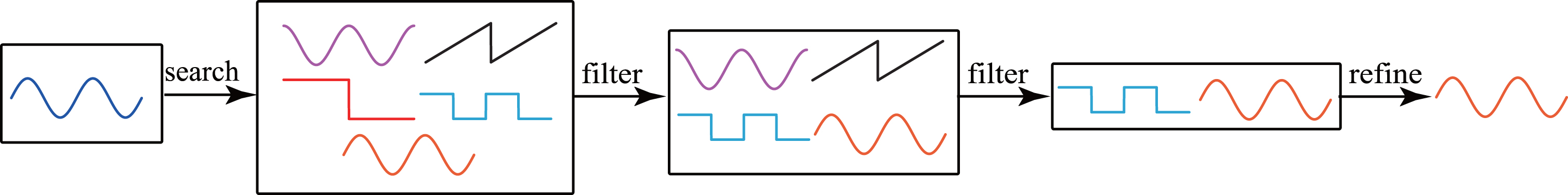
The framework diagram of using MDTW to find the nearest neighbor.

Table 1

Representing raw time series in different resolutions

Time series	2-resolution sequence	4-resolution sequence
a	(0, 0)	(0.64,-0.64,0.64,-0.64)
b	(0, 0)	(0, 0, 0, 0)
c	(0, 0)	(-0.5, 0.5, -0.5, 0.5)
d	(1, -1)	(1, 1, -1, -1)
e	(0, 0)	(0.64,-0.64,0.64,-0.64)
f	(0, 0)	(0.64,-0.64,0.64,-0.64)

3.3 The formal statement of MDTW

To significantly accelerate the NN-DTW, we must find a way to reduce the number of DTW computations. This is critical because each DTW computation takes quadratic time. MDTW uses the filters-and-refine framework to prune off a significant fraction of DTW computations so that the algorithm does not need to calculate the distance between query and all time series. In the following, a formal and detailed description of MDTW is presented. We list notations frequently used in this paper in Table 2.

Table 2
The notations frequently used in this paper

Notation Definition

q The query time series

N The size of time series dataset

D The time series dataset of N instances

D _i The time series D_i in D

n The length of time series

M The number of approximate levels

K = (K₁, K₂, . . . , K_M) Resolution vector: 1 < K₁ < K₂ < . . . < K_M < n

$\hat{D} [D_{j}]$ The K_i-resolution sequence of D_j

$\hat{D} [K_{i}]$ All K_i-resolution sequences in D

T = (T₁, T₂, . . . , T_M) Filter vector: 1 < T_M < T_M-1 < . . . < T₁ < N

Notation	Definition
q	The query time series
N	The size of time series dataset
D	The time series dataset of N instances
D _i	The time series D_i in D
n	The length of time series
M	The number of approximate levels
K = (K₁, K₂, . . . , K_M)	Resolution vector: 1 < K₁ < K₂ < . . . < K_M < n
$\hat{D} [D_{j}]$	The K_i-resolution sequence of D_j
$\hat{D} [K_{i}]$	All K_i-resolution sequences in D
T = (T₁, T₂, . . . , T_M)	Filter vector: 1 < T_M < T_M-1 < . . . < T₁ < N

Given a dataset D of N time series ${D_{i}}_{i = 1}^{N}$ , where each D_i is a time series of length n, we first define the resolution vector K of M integers (K₁, K₂, . . . , K_M), in which 1 < K₁ < K₂ < . . . < K_M < n. For all K_i ∈ K, we obtain $\hat{D} [K_{i}]$ by calculating K_i-resolution sequence of each time series in D. Formally, $\hat{D} [K_{i}]$ is denoted as $\hat{D} [K_{i}] = {\hat{D} [K_{i}] [D_{1}], \hat{D} [K_{i}] [D_{2}], . . ., \hat{D} [K_{i}] [D_{N}]},$ in which $\hat{D} [K_{i}] [D_{j}]$ is the K_i-resolution sequence of time series D_j. As $\hat{D} [K_{i}]$ is used for all queries, the computation of $\hat{D} [K_{i}]$ is one-off pre-processing for MDTW. Algorithm 1 gives the description of pre-processing step in MDTW.

The time complexity of Algorithm 1 is O (NMn). Note that when amortized over large numbers of time series queries, the overhead of pre-processing will be relatively minor. We then define a filter vector T of M integers (T₁, T₂, . . . , T_M), in which 1 < T_M < T_M-1 < . . . < T₁ < N. The filter vector represents that at i-th level, MDTW only preserves the T_i-nearest neighbors and prunes off the remaining data. We also use DTW distance to measure the similarity at each resolution.

Algorithm 1 The pseudo code of the pre-processing step of the MDTW

Require:

M: the number of approximate levels;

K: resolution vector K = (K₁, K₂, ..., K_M);

D: the time series dataset;

Ensure:

$\hat{D}$ : resolution sequences of each time series at each resolution;

1: for each K_i ∈ K do

2: for each time series D_j ∈ D do

3: temp ← K_i-resolution sequence of D_j;

4: $\hat{D} [K_{i}] [D_{j}] = temp$ ;

5: end for

6: end for

7: return $\hat{D}$ ;

We conclude a procedure of MDTW as shown in Algorithm 2. The filters-and-refine approach is used in Algorithm 2, which aims at reducing the number of exact DTW evaluations by using a computationally efficient strategy. In the filters stage (line 1-11), we first initialize the candidateSet with all time series in D (line 1). The K_i-resolution sequence of the query time series at i-th level is computed in line 3. Then we calculate all DTW distances between query and every time series in candidateSet at i-th level (line 4-8), and only preserve the T_i-nearest neighbors while removing others from candidateSet (line 9-10). To further filter out more time series data, we refine these candidates in a more refined resolution. The process of refining and calculating is continued until all M levels are evaluated (line 2). We note that compared to other time series, the remaining T_M time series are more likely to be the nearest neighbor of query time series.

In the refine stage (line 12-21), MDTW examines the 1-nearest neighbor by calculating the actual DTW distance at the original resolution among the remaining T_M time series. In MDTW, many DTW computations can be calculated in low-dimensional space. Therefore, the query processing is accelerated.

3.4 Time complexity analysis

As described in Section 2.2, there are dozens of methods for accelerating NN-DTW. Although such methods can be faster than traditional NN-DTW in the best case, some of these methods, such as the lower bound techniques, degenerate to sequential scan in the worst case. In contrast, we will show that the performance of the MDTW is completely independent of the dataset and can always be faster than NN-DTW.

Algorithm 2 The pseudo code of the query procedure of the MDTW

Require:

q: query time series;

M: the number of approximate levels;

T : filter vector T = (T₁, T₂, ..., T_M);

K: resolution vector K = (K₁, K₂, ..., K_M);

D: the time series dataset D = {D₁, D₂, ..., D_N};

$\hat{D}$

Ensure:

res: the nearest neighbor of query

1: candidateSet← all time series of D;

2: for i = 1 to M do

3: ${\hat{q}}_{K_{i}} \leftarrow$ K_i-resolution sequence of query q;

4: DTW _ res = [];

5: for each time series D_j ∈ candidateSet do

6: $temp = DTW ({\hat{q}}_{K_{i}}, \hat{D} [K_{i}] [D_{j}])$ ;

7: DTW _ res . add (temp);

8: end for

9: newCandidateSet = sort (DTW _ res, T_i);

10: candidateSet = newCandidateSet;

11: end for

12: best _ so _ far← + ∞;

13: res ← null;

14: for each time series D_i ∈ candidateSet do

15: temp = DTW (q, D_i);

16: if temp < best _ so _ far then

17: best _ so _ far = temp;

18: res = D_i;

19: end if

20: end if

21: return res;

We give some complexity analysis of MDTW outlined in Algorithm 2. At the 1-th level, MDTW costs $O ({NK}_{1}^{2})$ operations to calculate DTWs. At the i-th level (i > 1), there are T_i-1 time series of length K_i need to be calculated DTWs; thus, the complexity is $O (T_{i - 1} K_{i}^{2})$ . In the refine stage, MDTW costs O (T_Mn²) operations to find the nearest neighbor. Thus, MDTW costs

$C_{MDTW} = O ({NK}_{1}^{2} + \sum_{i = 1}^{M - 1} T_{i} K_{i + 1}^{2} + T_{M} n^{2})$ (1)

operations to calculate DTWs.

Suppose that cK_M = n and bT₁ = N, in which the value of c can be considered as the compression rate, which is the ratio of the length of the original time series (n) to the length of its K_M-resolution sequence (K_M). Similarly, b is the filter rate, which is the ratio of the the size of time series dataset (N) to the size of the remaining candidateSet (T₁) in the first filter-stage. By introducing c and b, we have $1 < K_{1} < K_{2} < . . . < \frac{n}{c} < n$ (2) and $1 < T_{M} < T_{M - 1} < . . . < \frac{N}{b} < N .$ (3) Inserting (2) and (3) in (1), we get $\begin{matrix} C_{MDTW} & = O ({NK}_{1}^{2} + \sum_{i = 1}^{M - 1} T_{i} K_{i + 1}^{2} + T_{M} n^{2}) \\ \leq O (N (\frac{n}{c})^{2} + (M - 1) \frac{N}{b} (\frac{n}{c})^{2} + \frac{N}{b} n^{2}) \\ = O ((\frac{N}{c^{2}} + \frac{N (M - 1)}{{bc}^{2}} + \frac{N}{b}) n^{2}) \\ = O (\frac{b + (M - 1) + c^{2}}{{bc}^{2}} {Nn}^{2}) . \end{matrix}$ (4) In NN-DTW, it costs $C_{NN - DTW} = O ({Nn}^{2})$ (5) operations to compute the DTW distances between query and all time series in D. Thus, the speedup obtained by MDTW should be greater than $O ({Nn}^{2}) / O (\frac{b + (M - 1) + c^{2}}{{bc}^{2}} {Nn}^{2})$ which is $Speedup = O (\frac{{bc}^{2}}{b + M - 1 + c^{2}}) .$ (6) In practice, M is always a small value, and b and c have the same order of magnitude. Thus, we can write (6) as $Speedup \approx O (b) .$ (7)

Note that the purpose of introducing b and c is to help us analyze the time complexity of the MDTW; otherwise, it is very difficult to establish the relationship between Equation 1 and Equation 5.

Equation 7 is a worst case bound, which demonstrates that MDTW performs faster than NN-DTW. The astute reader will note that, in our analysis, the time complexity of online transformation (line 3) and sort function (line 9) is omitted. However, for high dimensional time series, this cost is relatively minor and the main part of time complexity of MDTW is calculating DTW distances. Therefore we can reasonably ignore the cost of online transformation and sort function.

3.5 Combining with the state-of-the-art

MDTW focuses on reducing the total number of expensive exact DTW computations. However, MDTW still needs to calculate the exact DTWs between q and the remaining T_M time series. The simplest way to implement the refine stage is to compute the DTWs using traditional DTW distance calculation method [8]. However the traditional method involves quadratic time complexity; thus, even being performed only to the few time series, the refine stage still could be computationally expensive.

To make MDTW even faster, in this paper, we embed a recently proposed method, prunedDTW [40], into the MDTW procedure. Specifically, we adapt the prunedDTW algorithm to compute the DTW distance in Algorithm 2 (line 15). We choose prunedDTW for three main reasons: (1) prunedDTW is an exact algorithm. For two arbitrarily chosen time series A and B, we have prunedDTW (A, B) = DTW (A, B) . (2) prunedDTW has no parameters. This property is consistent with our purpose of designing MDTW. (3) prunedDTW can improve the efficiency of the DTW computation. Thus, we can speed up the refine stage.

Although combining with prunedDTW is just a small trick, in Section 4, we demonstrate that this small trick can speed up the MDTW from one to five times.

4 Experimental evaluation

We carry out an extensive set of experiments to verify the efficiency and effectiveness of the proposed method for TSC. This section reports and analyzes the experimental results. We implemented all methods in MATLAB (version R2019b), and performed all experiments using Windows 10 enterprise with 2.60 GHz and 16 GB memory.

4.1 Experimental Setup

4.1.1 Datasets

We conduct experiments on 18 representative datasets collected from the UCR archive [10]. Table 3 shows detailed information about the datasets. The selected datasets are collected from different application fields and are of various types, including sensor data, motion, image, simulated, and ECG data. The datasets vary widely in their time series lengths, number of classes, the size of the dataset, and the number of queries. Besides, compared with other UCR datasets, the chosen datasets can be regarded as large datasets that are generally larger in dimensionality or size. The small datasets can be performed relatively fast with the traditional methods; thus, in our experiments, we mainly focus on large datasets.

Table 3
Datasets descriptions and the pre-processing time (second) of MDTW for each dataset

Name Classes The size of the dataset The number of query Time series length Type Pre-processing time

Adiac 37 390 391 176 Image 0.0413

Chlo.Concen 3 467 3840 166 Sensor 0.0534

ElectricDevices 7 8926 7711 96 Device 0.7923

HandOutlines 2 370 1000 2709 Image 0.0529

Haptics 5 155 308 1092 Motion 0.0241

Non_Thorax1 42 1800 1965 750 ECG 0.1789

Non_Thorax2 42 1800 1965 750 ECG 0.1739

Phalanges.O.C 2 1800 858 80 Image 0.1587

Proximal.P.O.C 2 600 291 80 Image 0.0553

StarLightCurves 3 1000 8236 1024 Sensor 0.1212

Symbols 6 25 995 398 Image 0.0098

Two_Patterns 4 1000 4000 128 Simulated 0.1022

uWave_X 8 896 3582 315 Motion 0.0861

uWave_Y 8 896 3582 315 Motion 0.0880

uWave_Z 8 896 3582 315 Motion 0.0876

uWave.All 8 896 3582 945 Motion 0.1040

wafer 2 1000 6174 152 Sensor 0.0994

yoga 2 300 3000 426 Image 0.0339

Name	Classes	The size of the dataset	The number of query	Time series length	Type	Pre-processing time
Adiac	37	390	391	176	Image	0.0413
Chlo.Concen	3	467	3840	166	Sensor	0.0534
ElectricDevices	7	8926	7711	96	Device	0.7923
HandOutlines	2	370	1000	2709	Image	0.0529
Haptics	5	155	308	1092	Motion	0.0241
Non_Thorax1	42	1800	1965	750	ECG	0.1789
Non_Thorax2	42	1800	1965	750	ECG	0.1739
Phalanges.O.C	2	1800	858	80	Image	0.1587
Proximal.P.O.C	2	600	291	80	Image	0.0553
StarLightCurves	3	1000	8236	1024	Sensor	0.1212
Symbols	6	25	995	398	Image	0.0098
Two_Patterns	4	1000	4000	128	Simulated	0.1022
uWave_X	8	896	3582	315	Motion	0.0861
uWave_Y	8	896	3582	315	Motion	0.0880
uWave_Z	8	896	3582	315	Motion	0.0876
uWave.All	8	896	3582	945	Motion	0.1040
wafer	2	1000	6174	152	Sensor	0.0994
yoga	2	300	3000	426	Image	0.0339

4.1.2 The baseline methods

In this part, we give a short introduction of the baseline methods. We select these baseline methods for two main reasons: (1) they are all parameter-light classifiers, and few parameters need to be tuned. (2) They are widely used for TSC and can achieve state-of-the-art performance on many datasets.

NN-DTW is one of the benchmark methods for TSC. It uses brute-force strategy to find the nearest neighbor.

Weighted DTW (WDTW) [17], shapeDTW [51] and Complexity-Invariant DTW (CIDTW) [3] are three popular DTW variants for solving TSC problem and they improve the performance of DTW significantly.

Move-Split-Merge (MSM) [41] and Edit Distance with Real Penalty (ERP) [9] are two well-established similarity measures for time series and are widely used in instance-based framework.

In addition to the above algorithms, three techniques of accelerating NN-DTW procedure are also considered as baseline methods to demonstrate the efficiency of the MDTW.

PDTW [20] shares some similarities with our method. However, only one coarse resolution is used and the nearest neighbor is calculated at this resolution. Thus, the classification accuracy is unsatisfactory.

FTW+prunedDTW is a combination of prunedDTW [40] and FTW [31]. FTW+prunedDTW uses the prunedDTW to calculate the DTW distance and uses the lower bound presented in FTW to reduce the number of prunedDTW computations.

MDTW+prunedDTW is the method described in Section 3.5. In this Section, we will show that MDTW+prunedDTW can make MDTW even faster.

4.1.3 Parameter setup

In MDTW, the number of approximate levels M, the resolution vector K and the filter vector T should be considered before the evaluation. However, these parameters can be determined arbitrarily, and fine-tuning is not required for various datasets. Thus, in our next experiments, we set the same parameters for all datasets. Specifically, we set M = 2, K = (10, 20) and $T = (\frac{N}{10}, \frac{N}{100})$ . We note that this setting does achieve a relatively good classification accuracy over all the datasets. As for PDTW, we set $K = ⌈ \frac{n}{8} ⌉$ to avoid tuning parameter manually.

4.2 Pre-processing time

As described in algorithm 1, the time series in the dataset need to be approximated in different resolutions before the query procedure is executed. In this experiment, we evaluate the time cost of the pre-processing stage in MDTW approach.

Table 3 shows the pre-processing time (in seconds) of the MDTW on different datasets. It can be found that the pre-processing time is very small (less than one second). For example, the pre-processing time of MDTW on the ElectricDevices dataset with 8926 instances is only 0.7923 second. It is an important characteristic in many real-time applications because the overhead of the pre-processing step can be ignored.

4.3 Efficiency

This subsection shows the evaluation of the efficiency of each approach against NN-DTW in classifying query time series. For each dataset, the speedup rate is reported. Assume that t₁ is the query processing time for NN-DTW and t₂ is the query processing time for a particular method Θ, then the speedup rate of the method Θ is t₁/t₂. Fig. 4 shows the speedup rate of different methods on the UCR datasets. Note that the time complexity of the shapeDTW is too high and we can not obtain its specific query time on our laptop; thus, we do not list its speedup rate.

Fig. 4

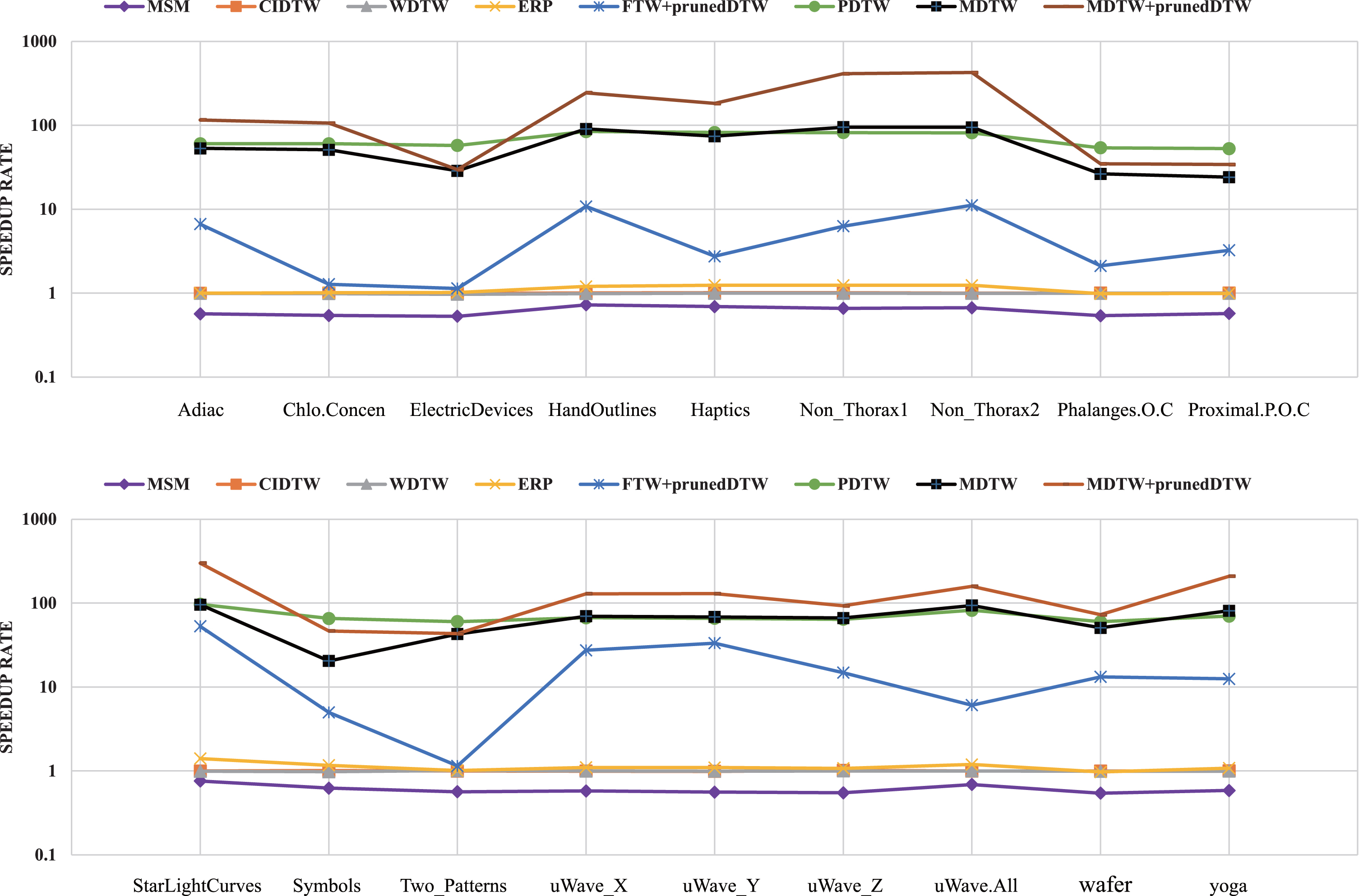
The speedup rate of different methods on the UCR datasets.

Fig. 4 illustrates that the MSM demonstrates poor result (the speedup rate is smaller than 1), and its query efficiency is worse than other methods. The CIDTW, WDTW and ERP are all quadratic-time algorithms, and as shown in Fig. 4, they have a similar query processing time as DTW under the nearest neighbor classifier (the speedup rate is close to 1). Furthermore, it can be clearly seen that NN-DTW spends much more time than MDTW, which demonstrates that MDTW can speed up NN-DTW as we expected. Specifically, MDTW achieves 20 to 95 faster than NN-DTW. Besides, it can be noted that MDTW+prunedDTW performs faster than MDTW and FTW+prunedDTW from 1 to 5 times and 4 to 85 times, respectively. Thus, we verify that when MDTW and prunedDTW are combined, MDTW+prunedDTW significantly outperforms both MDTW and prunedDTW individually.

Fig. 4 also shows that PDTW performs faster than NN-DTW and FTW+prunedDTW. Thus, PDTW can be regarded as the most competitive method among all the baseline methods. The Wilcoxon signed-rank test is conducted to demonstrate the superiority of the proposed approaches. Specifically, the p-value between PDTW and MDTW is 0.2668 > 0.05, which shows that the difference is not significant with the confidence of 95%; thus, the efficiency of MDTW is comparable to PDTW. The p-value between PDTW and MDTW+prunedDTW is 0.0043 < 0.05; thus our proposed improved MDTW method performs significantly better than PDTW and can be regarded as the most efficient algorithm among all competitors.

4.4 Effectiveness

In this subsection, we compare MDTW with baseline algorithms to evaluate the effectiveness of MDTW. The classification accuracy is reported. The experiment results of the PDTW are implemented by ourselves, and the results of the other six baseline approaches can be obtained in [1, 48]. Table 4 presents the classification results and average accuracy. Note that MDTW+prunedDTW and FTW+prunedDTW are not listed in Table 4 because they have the same accuracy with MDTW and NN-DTW, respectively.

Table 4
The results of the classification accuracy

Name MDTW NN-DTW CIDTW ERP MSM PDTW WDTW shapeDTW

Adiac 0.575 0.604 0.624 0.609 0.627 0.550 0.606 0.731

Chlo.Concen 0.643 0.648 0.649 0.660 0.628 0.586 0.649 0.645

ElectricDevices 0.596 0.601 0.616 0.654 0.659 0.559 0.613 0.600

HandOutlines 0.800 0.798 0.862 0.884 0.876 0.797 0.870 0.794

Haptics 0.390 0.377 0.425 0.370 0.442 0.373 0.370 0.377

Non_Thorax1 0.818 0.791 0.837 0.825 0.816 0.775 0.816 0.781

Non_Thorax2 0.866 0.865 0.879 0.895 0.883 0.849 0.885 0.860

Phalanges.O.C 0.749 0.728 0.762 0.760 0.752 0.696 0.747 0.739

Proximal.P.O.C 0.763 0.784 0.790 0.795 0.790 0.739 0.784 0.794

StarLightCurves 0.882 0.907 0.918 0.862 0.868 0.890 0.895 0.900

Symbols 0.902 0.950 0.941 0.921 0.949 0.939 0.950 0.961

Two_Patterns 1.000 1.000 0.881 0.942 0.947 0.994 1.000 0.999

uWave_X 0.738 0.727 0.790 0.771 0.769 0.750 0.774 0.737

uWave_Y 0.644 0.634 0.723 0.679 0.702 0.643 0.693 0.642

uWave_Z 0.654 0.658 0.706 0.687 0.700 0.662 0.676 0.662

uWaveAll 0.932 0.892 0.963 0.954 0.963 0.913 0.966 0.942

wafer 0.977 0.980 0.994 0.995 0.997 0.979 0.997 0.990

yoga 0.825 0.836 0.844 0.847 0.865 0.826 0.853 0.883

Average accuracy 0.764 0.766 0.789 0.784 0.791 0.751 0.786 0.780

Name	MDTW	NN-DTW	CIDTW	ERP	MSM	PDTW	WDTW	shapeDTW
Adiac	0.575	0.604	0.624	0.609	0.627	0.550	0.606	0.731
Chlo.Concen	0.643	0.648	0.649	0.660	0.628	0.586	0.649	0.645
ElectricDevices	0.596	0.601	0.616	0.654	0.659	0.559	0.613	0.600
HandOutlines	0.800	0.798	0.862	0.884	0.876	0.797	0.870	0.794
Haptics	0.390	0.377	0.425	0.370	0.442	0.373	0.370	0.377
Non_Thorax1	0.818	0.791	0.837	0.825	0.816	0.775	0.816	0.781
Non_Thorax2	0.866	0.865	0.879	0.895	0.883	0.849	0.885	0.860
Phalanges.O.C	0.749	0.728	0.762	0.760	0.752	0.696	0.747	0.739
Proximal.P.O.C	0.763	0.784	0.790	0.795	0.790	0.739	0.784	0.794
StarLightCurves	0.882	0.907	0.918	0.862	0.868	0.890	0.895	0.900
Symbols	0.902	0.950	0.941	0.921	0.949	0.939	0.950	0.961
Two_Patterns	1.000	1.000	0.881	0.942	0.947	0.994	1.000	0.999
uWave_X	0.738	0.727	0.790	0.771	0.769	0.750	0.774	0.737
uWave_Y	0.644	0.634	0.723	0.679	0.702	0.643	0.693	0.642
uWave_Z	0.654	0.658	0.706	0.687	0.700	0.662	0.676	0.662
uWaveAll	0.932	0.892	0.963	0.954	0.963	0.913	0.966	0.942
wafer	0.977	0.980	0.994	0.995	0.997	0.979	0.997	0.990
yoga	0.825	0.836	0.844	0.847	0.865	0.826	0.853	0.883
Average accuracy	0.764	0.766	0.789	0.784	0.791	0.751	0.786	0.780

From Table 4, it is clearly seen that in general, no single method outperforms all other methods for all datasets. Furthermore, we discover that MDTW, compared to NN-DTW, can even achieve improved classification accuracy on some datasets, like Haptics. It may be because although DTW does achieve a global minimal score, the alignment process itself takes no local structural information into account, possibly resulting in an alignment with little semantic meaning [51], which may lead to misclassification. However, MDTW takes local structural information into account by using mean operation on subsequences. Therefore, the pathological nearest neighbor calculated by NN-DTW may be filtered out by MDTW in a coarse resolution. Consequently, a reasonable nearest neighbor can be found by MDTW, and then the accuracy is improved. We also do the Wilcoxon signed rank test between the MDTW and NN-DTW in terms of accuracy. The p-value is 0.7582 > 0.05, which demonstrates that the difference between MDTW and NN-DTW is not significant with the confidence of 95%.

The results in Table 4 show that the classification accuracy of PDTW is not good enough. Our method achieves better accuracy than PDTW on 12 datasets out of 18, and the p-value of Wilcoxon signed rank test between PDTW and MDTW in terms of accuracy is 0.0474 < 0.05. However, five strong competitors (i.e., CIDTW, ERP, MSM, WDTW and shapeDTW) outperform our method MDTW in most cases and the p-value >0.05. It is understandable because these methods can be considered as state-of-the-art methods for TSC and are hard to beat. We acknowledge this weakness. Nevertheless, it is worth noting that there is no significant difference between our algorithm and the state-of-the-art in average accuracy, with very small losses (<3%). In addition, we note that in some datasets such as Chlo.Concen and Two_Patterns, the MDTW can even perform better than state-of-the-art or achieve comparative performance (losses <1%).

The optimal classification results are not always required in many real-time applications in which the responsiveness is more critical than classification accuracy and sub-optimal results with quality guarantee are also acceptable. The experiment results show that our method can improve the classification efficiency significantly and achieve comparative performance with the state-of-the-art, with very small losses in accuracy. For example, MDTW can achieve 32 to 140 faster than MSM while having minor losses in average accuracy (2.7%). Thus, in the situations where the responsiveness is more important than the accuracy, e.g., when in real-time analytics, MDTW can be considered as a good solution.

4.5 Sensitivity analysis

In the previous subsection, we report the classification accuracy and the speedup rate under a fixed parameter setting. Nevertheless, the performance robustness under various parameter settings deserves our attention. Thus, in this part, we explore the effects of parameters on classification results and speedup rate. To see how them changes, we vary one parameter at a time and maintain other parameters fixed. We use the dataset wafer as the example here to evaluate the performance sensitivity of MDTW to each parameter.

In our previous experiments, for dataset wafer, we set K = (10, 20) and $T = (\frac{N}{10}, \frac{N}{100}) = (100, 10)$ . In this evaluation, the value of K₁ is in the range of 5 to 15 and the value of K₂ ranges from 15 to 25. As for T, we set T₁ in the range of 95 to 105 and T₂ in the range of 5 to 15. All parameters with fixed step size 1.

Fig. 5 reports the classification accuracy and speedup rate under different input values of T₁, T₂, K₁, K₂. From Fig. 5(a)-(d), we find the accuracy nearly keeps stable, which suggests that our method is largely insensitive to the resolution vector K and the filter vector T. It is because even if the parameters are different, in most cases, after consequent filtering out dissimilar time series at each resolution level, the final candidateSet still contains the actually nearest neighbor time series. So in the refine-stage, the MDTW can obtain the same result. This is a beneficial characteristic because it means that we do not require any fine-tuning for a dataset. Besides, from Fig. 5(e)-(h) we find that T₂ and K₁ greatly affect the speedup rate while T₁ and K₂ have little effect on the speedup rate. Thus, in practice, a higher efficiency can be obtained by changing parameters T₂ and K₁. Note that although the speedup rate is affected by the T₂ and K₁, the classification accuracy is insensitive to the parameters.

Fig. 5

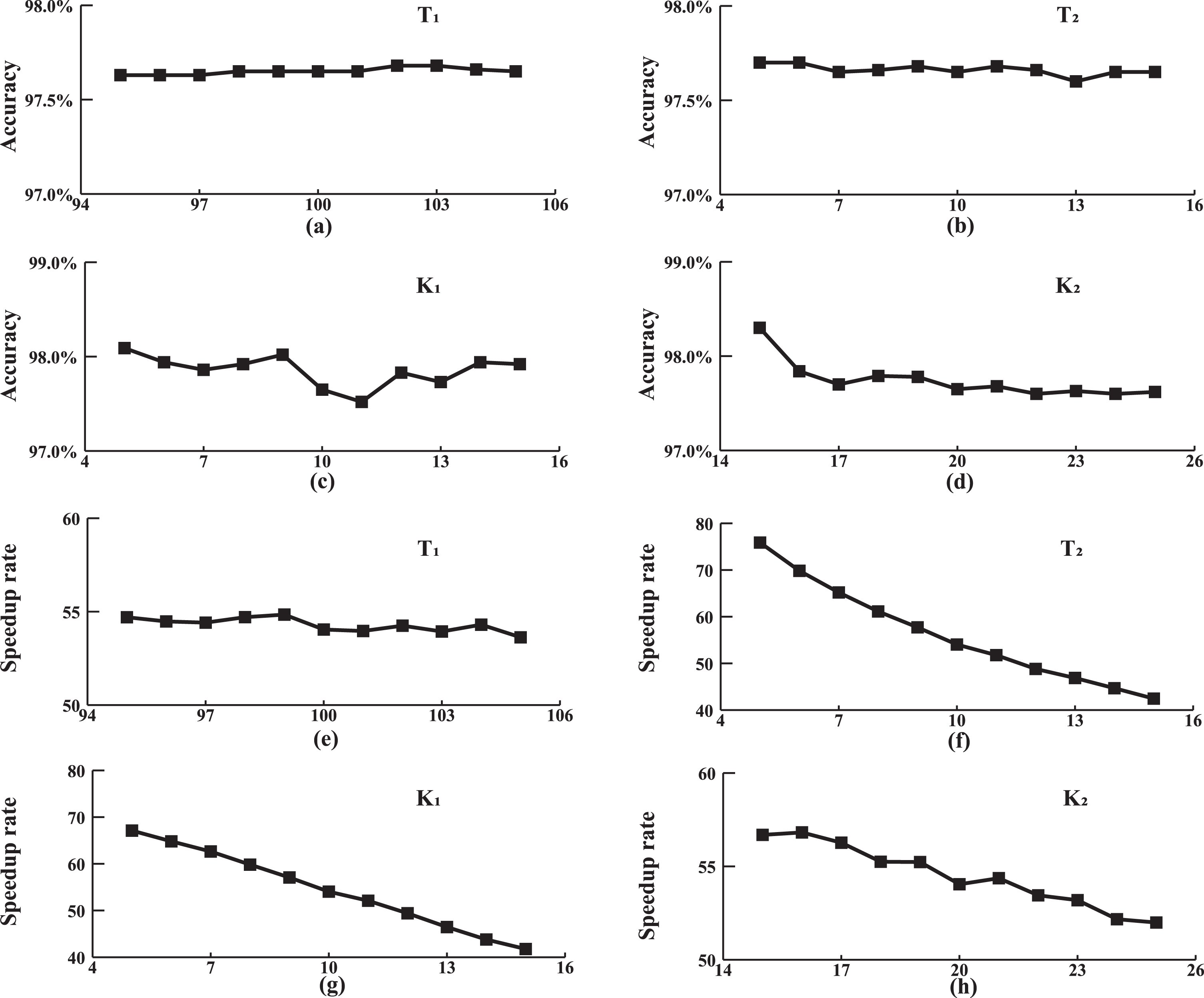
The classification accuracy and the speedup rate of MDTW under different input values of T₁, T₂, K₁, K₂. The results show that the classification accuracy is not sensitive to parameters T and K, and the speedup rate is approximately linear by T₂ and K₁.

5 Conclusion and future work

In this paper, we propose a parameter-light method, called MDTW, for time series classification, and present its effectiveness and computational efficiency compared with existing methods. Experimental results show that MDTW achieves substantial speedups and comparative accuracy performance compared with state-of-the-art methods. Besides, we do the experiments to show that our approach is largely insensitive to parameters. We also provide a strategy to make MDTW even faster. Specifically, we embed the prunedDTW technique into the MDTW procedure. As shown in experimental results, MDTW+prunedDTW can speed up the MDTW from one to five times.

The discussion in this paper has focused on DTW distance. However, the idea behind MDTW can be applied to most time series similarity measures. In future research, we will implement the idea for various similarity measures. It will be interesting to know the trade-off between efficiency and accuracy. Another meaningful direction is testing the impacts of different local descriptors on the time series classification accuracy.

References

Bagnall

, Lines

, Bostrom

, Large

and Keogh

, The great time series classification bake off: a review and experimental evaluation of recent algorithmic advances, Data Mining and Knowledge Discovery 31(3) (2017), 606–660.

Bagnall

, Lines

, Hills

and Bostrom

, Time-series classification with cote: the collective of transformation-based ensembles, IEEE Transactions on Knowledge and Data Engineering 27(9) (2015), 2522–2535.

Batista

G.E.

, Keogh

E.J.

, Tataw

O.M.

and MA De Souza

, Cid: an efficient complexityinvariant distance for time series, Data Mining and Knowledge Discovery 28(3) (2014), 634–669.

Baydogan

M.G.

, Runger

and Tuv

, A bag-of-features framework to classify time series, IEEE Transactions on Pattern Analysis and Machine Intelligence 35(11) (2013), 2796–2802.

Baydogan

M.G.

and Runger

, Time series representation and similarity based on local autopatterns, Data Mining and Knowledge Discovery 30(2) (2016), 476–509.

Baydogan

M.G.

, Runger

and Tuv

, A bag-of-features framework to classify time series, IEEE transactions on pattern analysis and machine intelligence 35(11) (2013), 2796–2802.

Bostrom

and Bagnall

, Binary shapelet transform for multiclass time series classification, In International conference on big data analytics and knowledge discovery, 257–269. Springer, (2015).

Selçuk Candan

, Rossini

, Wang

and Sapino

M.L.

, sdtw: computing dtw distances using locally relevant constraints based on salient feature alignments, Proceedings of the VLDB Endowment 5(11) (2012), 1519–1530.

Chen

and Ng

, On the marriage of lp-norms and edit distance. In Proceedings of the Thirtieth international conference on Very large data bases-Volume 30, pages 792–803. VLDB Endowment, (2004).

10.

Chen

, Keogh

, Hu

, Begum

, Bagnall

, Mueen

and Batista

, The ucr time series classification archive, (2015). www.cs.ucr.edu/ eamonn/time series data/.

11.

Chu

, Keogh

E.J.

, Hart

D.M.

and Pazzani

M.J.

, Iterative deepening dynamic time warping for time series, In SDM, (2002), pages 195–212.

12.

Deng

, Runger

, Tuv

and Vladimir

, A time series forest for classification and feature extraction, Information Sciences 239 (2013), 142–153.

13.

Deng

, Runger

, Tuv

and Vladimir

, A time series forest for classification and feature extraction, Information Sciences 239 (2013), 142–153.

14.

Esling

and Agon

, Time-series data mining, ACM Computing Surveys (CSUR) 45(1) (2012), 12.

15.

Grabocka

, Schilling

, Wistuba

and Schmidt-Thieme

, Learning time-series shapelets, In Proceedings of the 20th ACMSIGKDD international conference on Knowledge discovery and data mining, (2014), pages 392–401.

16.

Hills

, Lines

, Baranauskas

, Mapp

and Bagnall

, Classification of time series by shapelet transformation, Data Mining and Knowledge Discovery 28(4) (2014), 851–881.

17.

Jeong

Y.-S.

, Jeong

M.K.

and Omitaomu

O.A.

, Weighted dynamic time warping for time series classification, Pattern Recognition 44(9) (2011), 2231–2240.

18.

Keogh

, Chakrabarti

, Pazzani

and Mehrotra

, Dimensionality reduction for fast similarity search in large time series databases, Knowledge and information Systems 3(3) (2001), 263–286.

19.

Keogh

and Ratanamahatana

C.A.

, Exact indexing of dynamic time warping, Knowledge and Information Systems 7(3) (2005), 358–386.

20.

Keogh

E.J.

and Pazzani

M.J.

, Scaling up dynamic time warping for datamining applications, In Proceedings of the sixth ACM SIGKDD international conference on Knowledge discovery and data mining, pages 285–289. ACM, (2000).

21.

Kim

S.-W.

, Park

and Chu

W.W

, An index-based approach for similarity search supporting time warping in large sequence databases, In Proceedings 17th International Conference on Data Engineering, pages 607–614. IEEE, (2001).

22.

Kiranyaz

, Ince

and Gabbouj

, Real-time patient-specific ecg classification by 1-d convolutional neural networks, IEEE Transactions on Biomedical Engineering 63(3) (2015), 664–675.

23.

Nguyen

T.L.

, Gsponer

and Ifrim

, Time series classification by sequence learning in allsubsequence space, In 2017 IEEE 33rd international conference on data engineering (ICDE), pages 947–958. IEEE, (2017).

24.

Lin

, Keogh

, Wei

and Lonardi

, Experiencing sax: a novel symbolic representation of time series, Data Mining and Knowledge Discovery 15(2) (2007), 107–144.

25.

Lin

, Khade

and Li

, Rotation-invariant similarity in time series using bag-of-patterns representation, Intelligent Information Systems 39(2) (2012), 287–315.

26.

Lines

and Bagnall

, Time series classification with ensembles of elastic distance measures, Data Mining and Knowledge Discovery 29(3) (2015), 565–592.

27.

Lines

, Taylor

and Bagnall

, Time series classification with hive-cote: The hierarchical vote collective of transformation-based ensembles, ACM Transactions on Knowledge Discovery From Data 12(5) (2018), 52.

28.

Nwe

T.L.

, Dat

T.H.

and Ma

, Convolutional neural network with multi-task learning scheme for acoustic scene classification, In 2017 Asia-Pacific Signal and Information Processing Association Annual Summit and Conference (APSIPA ASC), (2017), pages 1347–1350.

29.

Rakthanmanon

and Keogh

, Fast-shapelets: A fast algorithm for discovering robust time series shapelets, In Proceedings of 11th SIAM International Conference on Data Mining, (2011).

30.

Raza

and Kramer

, Accelerating pattern-based time series classification: a linear time and space string mining approach, Knowledge and Information Systems 62(3) (2020), 1113–1141.

31.

Sakurai

, Yoshikawa

and Faloutsos

, Ftw: fast similarity search under the time warping distance, In Proceedings of the twenty-fourth ACM SIGMODSIGACT-SIGART symposium on Principles of database systems, pages 326–337. (2005).

32.

Salvador

and Chan

, Toward accurate dynamic time warping in linear time and space, Intelligent Data Analysis 11(5) (2007), 561–580.

33.

Schäfer

, The boss is concerned with time series classification in the presence of noise, Data Mining and Knowledge Discovery 29(6) (2015), 1505–1530.

34.

Schäfer

and Leser

, Fast and accurate time series classification with weasel. In Proceedings of the 2017 ACM on Conference on Information and Knowledge Management, pages 637–646. ACM, (2017).

35.

Schäfer

, The boss is concerned with time series classification in the presence of noise, Data Mining and Knowledge Discovery 29(6) (2015), 1505–1530.

36.

Schäfer

and Högqvist

, Sfa: a symbolic fourier approximation and index for similarity search in high dimensional datasets, In Proceedings of the 15th International Conference on Extending Database Technology, (2012), pages 516–527.

37.

Senin

and Malinchik

, Sax-vsm: Interpretable time series classification using sax and vector space model, In 2013 IEEE 13th International Conference on Data Mining, (2013), 1175–1180.

38.

Shannon

R.V.

, Zeng

F.-G.

, Kamath

, Wygonski

and Ekelid

, Speech recognition with primarily temporal cues, Science 270(5234) (1995), 303–304.

39.

Shifaz

, Pelletier

, Petitjean

and Webb

G.I.

, Ts-chief: a scalable and accurate forest algorithm for time series classification, Data Mining and Knowledge Discovery (2020), pages 1–34.

40.

Silva

D.F.

and Batista

G.E.

, Speeding up allpairwise dynamic timewarping matrix calculation, In Proceedings of the 2016 SIAM International Conference on Data Mining, pages 837–845. SIAM, (2016).

41.

Stefan

, Athitsos

and Das

, The move-split-merge metric for time series, IEEE transactions on Knowledge and Data Engineering 25(6) (2012), 1425–1438.

42.

Tan

C.W.

, Webb

G.I.

and Petitjean

, Indexing and classifying gigabytes of time series under time warping, In SIAM International Conference on Data Mining 2017 pages 282–290, (2017).

43.

Tran

T.M.

, Le

X.-M.T.

, Nguyen

H.T.

and Huynh

V.-N.

, A novel non-parametric method for time series classification based on k-nearest neighbors and dynamic time warping barycenter averaging, Engineering Applications of Artificial Intelligence 78 (2019), 173–185.

44.

Wang

, Chen

, Hao

, Peng

and Hu

, Deep learning for sensor-based activity recognition: A survey, Pattern Recognition Letters 119 (2018), 3–11.

45.

Wilcoxon

, Individual comparisons by ranking methods, Biometrics 1(6) (1945), 196–202.

46.

and Keogh

, Time series shapelets: a new primitive for data mining. In Proceedings of the 15th ACM SIGKDD international conference on Knowledge discovery and data mining, pages 947–956. ACM, (2009).

47.

B.-K.

, Jagadish

H.V.

and Faloutsos

, Efficient retrieval of similar time sequences under time warping, In Proceedings 14th International Conference on Data Engineering, pages 201–208. IEEE, (1998).

48.

Yuan

, Lin

, Zhang

and Wang

, Locally slope-based dynamic time warping for time series classification, In Proceedings of the 28th ACM International Conference on Information and Knowledge Management (2019), pages 1713–1722.

49.

Zhang

, Ding

and Sun

, A support vector regression model hybridized with chaotic krill herd algorithm and empirical mode decomposition for regression task, Neurocomputing (2020).

50.

Zhao

and Itti

, Classifying time series using local descriptors with hybrid sampling, IEEE Transactions on Knowledge and Data Engineering 28(3) (2016), 623–637.

51.

Zhao

and Itti

, Shapedtw: shape dynamic time warping, Pattern Recognition 74 (2018), 171–184.