Ensembles of classifiers based on dimensionality reduction

Abstract

We present a novel approach for the construction of ensemble classifiers based on dimensionality reduction. The ensemble members are trained based on dimension-reduced versions of the training set. In order to classify a test sample, it is first embedded into the dimension reduced space of each individual classifier by using an out-of-sample extension algorithm. Each classifier is then applied to the embedded sample and the classification is obtained via a voting scheme. We demonstrate the proposed approach using the Random Projections, the Diffusion Maps and the Random Subspaces dimensionality reduction algorithms. We also present a multi-strategy ensemble which combines AdaBoost and Diffusion Maps. A comparison is made with the Bagging, AdaBoost, Rotation Forest ensemble classifiers and also with the base classifier. Our experiments used seventeen benchmark datasets from the UCI repository. The results obtained by the proposed algorithms were superior in many cases to other algorithms.

Keywords

Ensembles of classifiers dimensionality reduction out-of-sample extension Random Projections Diffusion Maps Nyström extension

1. Introduction

Classifiers are predictive models which label data based on a training dataset $T$ whose labels are known a-priory. A classifier is constructed by applying an induction algorithm, or inducer, to $T$ – a process that is commonly known as training. Classifiers differ by the induction algorithms and training sets that are used for their construction. Common induction algorithms include nearest neighbors (NN), decision trees, Support Vector Machines (SVM) [64] and Artificial Neural Networks – to name a few. Since every inducer has its advantages and weaknesses, methodologies have been developed to enhance their performance. Ensemble classifiers are one of the most common ways to achieve that.

The need for dimensionality reduction techniques emerged in order to alleviate the so called curse of dimensionality [32]. In many cases, a high-dimensional dataset lies approximately on a low-dimensional manifold in the ambient space. Dimensionality reduction methods embed datasets into a low-dimensional space while preserving as much of the information conveyed by the dataset. The low-dimensional representation is referred to as the embedding of the dataset. Since the information is inherent in the geometrical structure of the dataset (e.g. clusters), a good embedding distorts the structure as little as possible while representing the dataset using a number of features that is substantially smaller than the dimension of the original ambient space. Furthermore, an effective dimensionality reduction algorithm also removes noisy features and inter-feature correlations. Due to its properties, dimensionality reduction is a common step in many machine learning applications in fields such as signal processing [53, 1, 2] and image processing [41].

1.1 Ensembles of classifiers

Ensembles of classifiers [36] mimic the human nature to seek advice from several people before making a decision where the underlying assumption is that combining the opinions will produce a decision that is better than each individual opinion. Several classifiers (ensemble members) are constructed and their outputs are combined – usually by voting or an averaged weighting scheme – to yield the final classification [46]. In order for this approach to be effective, two criteria must be met: accuracy and diversity [36]. Accuracy requires each individual classifier to be as accurate as possible i.e. individually minimize the generalization error. Diversity requires to minimize the correlation among the generalization errors of the classifiers. These criteria are contradictory since optimal accuracy achieves a minimum and unique error which contradicts the requirement of diversity. Complete diversity, on the other hand, corresponds to random classification which usually achieves the worst accuracy. Consequently, individual classifiers that produce results which are moderately better than random classification are suitable as ensemble members. In [42], “kappa-error” diagrams are introduced to show the effect of diversity at the expense of reduced individual accuracy.

In this paper we focus on ensemble classifiers that use a single induction algorithm, for example the nearest neighbor inducer. This ensemble construction approach achieves its diversity by manipulating the training set. A well known way to achieve diversity is by bootstrap aggregation (Bagging) [6]. Several training sets are constructed by applying bootstrap sampling (each sample may be drawn more than once) to the original training set. Each training set is used to construct a different classifier where the repetitions fortify different training instances. This method is simple yet effective and has been successfully applied to a variety of problems such as spam detection [67] and analysis of gene expressions [62].

The award winning Adaptive Boosting (AdaBoost) [22] algorithm provides a different approach for the construction of ensemble classifiers based on a single induction algorithm. This approach iteratively assigns weights to each training sample where the weights of the samples that are misclassified are increased according to a global error coefficient. The final classification combines the logarithm of the weights to yield the ensemble’s classification.

Rotation Forest [47] is one of the current state-of-the-art ensemble classifiers. This method constructs different versions of the training set by employing the following steps: First, the feature set is divided into disjoint sets on which the original training set is projected. Next, a random sample of classes is eliminated and a bootstrap sample is selected from every projection result. Principal Component Analysis [30] (see Section 1.2) is then used to rotate each obtained subsample. Finally, the principal components are rearranged to form the dataset that is used to train a single ensemble member. The first two steps provide the required diversity of the constructed ensemble.

Multi-strategy ensemble classifiers [49] aim at combining the advantages of several ensemble algorithms while alleviating their disadvantages. This is achieved by applying an ensemble algorithm to the results produced by another ensemble algorithm. Examples of this approach include multi-training SVM (MTSVM) [38], MultiBoosting [65] and its extension using stochastic attribute selection [66].

Successful applications of the ensemble methodology can be found in many fields, for example, recommender systems [55], fMRI decoding [8], manufacturing [48] and eye pupil localization [43].

1.2 Dimensionality reduction

The theoretical foundations for dimensionality reduction were established by Johnson and Lindenstrauss [33] who proved its feasibility. Specifically, they showed that $N$ points in an $N$ dimensional space can almost always be projected onto a space of dimension $C\log N$ with control over the ratio of distances and the error (distortion). Bourgain [5] showed that any metric space with $N$ points can be embedded by a bi-Lipschitz map into an Euclidean space of $\log N$ dimension with a bi-Lipschitz constant of $\log N$ . Various randomized versions of these theorems were successfully applied to a variety of problem, for example, protein mapping [40] and reconstruction of frequency sparse signals [9, 17].

The dimensionality reduction problem can be formally described as follows. Let

$\Gamma=\left\{x_{i}\right\}_{i=1}^{N}$ (1)

be the original high-dimensional dataset given as a set of column vectors where $x_{i}\in\mathbb{R}^{n}$ , $n$ is the dimension of the ambient space and $N$ is the size of the dataset. All dimensionality reduction methods embed the vectors into a lower dimensional space $\mathbb{R}^{q}$ where $q\ll n$ . Their output is a set of column vectors in the lower dimensional space

$\widetilde{\Gamma}=\left\{\widetilde{x}_{i}\right\}_{i=1}^{N},\,\widetilde{x}_% {i}\in\mathbb{R}^{q}$ (2)

where $q$ is chosen such that it approximates the intrinsic dimensionality of $\Gamma$ [27]. We refer to the vectors in the set $\widetilde{\Gamma}$ as the embedding vectors.

Dimensionality reduction techniques employ two approaches: feature selection and feature extraction. Feature selection methods reduce the dimensionality by choosing $q$ features from the feature vectors according to given criteria. The same features are chosen from all vectors. Feature extraction methods, on the other hand, derive features which are functions of the original features.

Dimensionality techniques can also be divided into global and local methods. The former derive embeddings in which all points satisfy a given criterion. Examples for global methods include:

•

Principal Component Analysis (PCA) [30] which finds a low-dimensional embedding of the data points that best preserves their variance as measured in the ambient (high-dimensional) space;

•

Kernel PCA (KPCA) [56] which is a generalization of PCA that is able to preserve non-linear structures. This ability relies on the kernel trick i.e. any algorithm whose description involves only dot products and does not require explicit usage of the variables can be extended to a non-linear version by using Mercer kernels [57]. When this principle is applied to dimensionality reduction it means that non-linear structures correspond to linear structures in some high-dimensional space. These structures can be detected by linear methods using kernels.

•

Multidimensional scaling (MDS) [34, 14] algorithms which find an embedding that best preserves the inter-point distances among the vectors according to a given metric. This is achieved by minimizing a loss/cost stress function that measures the error between the pairwise distances of the embedding and their corresponding distances in the original dataset.

•

ISOMAP [61] which applies MDS using the geodesic distance metric. The geodesic distance between a pair of points is defined as the length of the shortest path connecting these points that passes only through points in the dataset.

•

Random projections [9, 17] in which every high-dimensional vector is projected onto a random matrix in order to obtain the embedding vector. This method is described in details in Section 4.

Contrary to global methods, local methods construct embeddings in which only local neighborhoods are required to meet a given criterion. The global description of the dataset is derived by the aggregation of the local neighborhoods. Common local methods include Local Linear Embedding (LLE) [51], Laplacian Eigenmaps [3], Hessian Eigenmaps [18], Local tangent space alignment [69], Discriminative Locality Alignment (DLA) [68] and Diffusion Maps [11, 52] which is used in this paper and is described in Section 3.

A key aspect of dimensionality reduction is how to efficiently embed a new point into a given dimension-reduced space. This is commonly referred to as out-of-sample extension where the sample stands for the original dataset whose dimensionality was reduced and does not include the new point. An accurate embedding of a new point requires the recalculation of the entire embedding. This is impractical in many cases, for example, when the time and space complexity that are required for the dimensionality reduction is quadratic (or higher) in the size of the dataset. An efficient out-of-sample extension algorithm embeds the new point without recalculating the entire embedding - usually at the expense of the embedding accuracy.

The Nyström extension [44] algorithm, which is used in this paper, embeds a new point in linear time using the quadrature rule when the dimensionality reduction involves eigen-decomposition of a kernel matrix. Algorithms such as Laplacian Eigenmaps, ISOMAP, LLE, and Diffusion Maps are examples that fall into this category and, thus, the embeddings that they produce can be extended using the Nyström extension [26, 4]. A formal description of the Nyström extension is given in Section 3.3.

The main contribution of this paper is a novel framework for the construction of ensemble classifiers based on dimensionality reduction and out-of-sample extension. This approach achieves both the diversity and accuracy which are required for the construction of an effective ensemble classifier and it is general in the sense that it can be used with any inducer and any dimensionality reduction algorithm as long as it can be coupled with an out-of-sample extension method that suits it.

The rest of this paper is organized as follows. In Section 2 we describe the proposed approach. In Sections 3–5 we introduce ensemble classifiers that are based on the Diffusion Maps, random projections and random subspaces dimensionality reduction algorithms, respectively. Experimental results are given in Section 6. We conclude and describe future work in Section 7.

2. Dimensionality reduction ensemble classifiers

The proposed approach achieves the diversity requirement of ensemble classifiers by applying a given dimensionality reduction algorithm to a given training set using different values for its input parameters. An input parameter that is common to all dimensionality reduction techniques is the dimension of the embedding space. In order to obtain sufficient diversity, the dimensionality reduction algorithm that is used should incorporate additional input parameters or, alternatively, incorporate a randomization step. For example, the Diffusion Maps [11] dimensionality algorithm uses an input parameter that defines the size of the local neighborhood of a point. Variations of this notion appear in other local dimensionality reduction methods such as LLE [51] and Laplacian Eigenmaps [3]. The Random Projections [17] (Section 4) and Random Subspaces [28, 50] (Section 5) methods, on the other hand, do not include input parameters other than the dimensionality of the embedding space. However, they incorporate a randomization step which diversifies the data (this approach already demonstrated good results using Random Projections in [54] and we extend them in this paper). In this sense, PCA is not suitable for the proposed framework since it does not include a randomization step and the only input parameter it has is the dimension of the embedding space (this parameter can also be set according to the total amount of variance of the original dataset that the embedding is required to maintain). Thus, PCA offers no way to diversify the data. On the other hand, dimensionality reduction algorithms that are suitable for the proposed method include ISOMAP [61], LLE [51], Hessian LLE [18], Local tangent space alignment [69] and Discriminative Locality Alignment (DLA) [68]. These methods are suitable since they require as input the number of nearest neighbors to determine the size of the local neighborhood of each data point. Laplacian Eigenmaps [3] and KPCA [56] are also suitable for the proposed framework as they include a continuous input variable to determine the radius of the local neighborhood of each point.

After the training sets are produced by the dimensionality reduction algorithms, each set is used to train a classifier to produce one of the ensemble members. The training process is illustrated in Fig. 1.

Figure 1.

Ensemble training.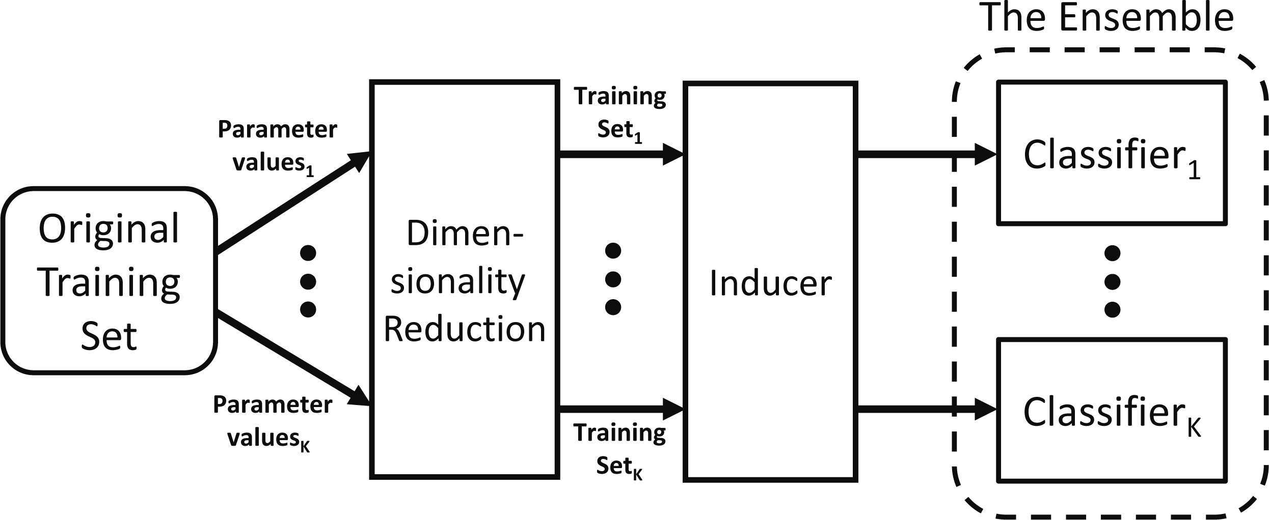

Figure 2.

Classification process of a test sample.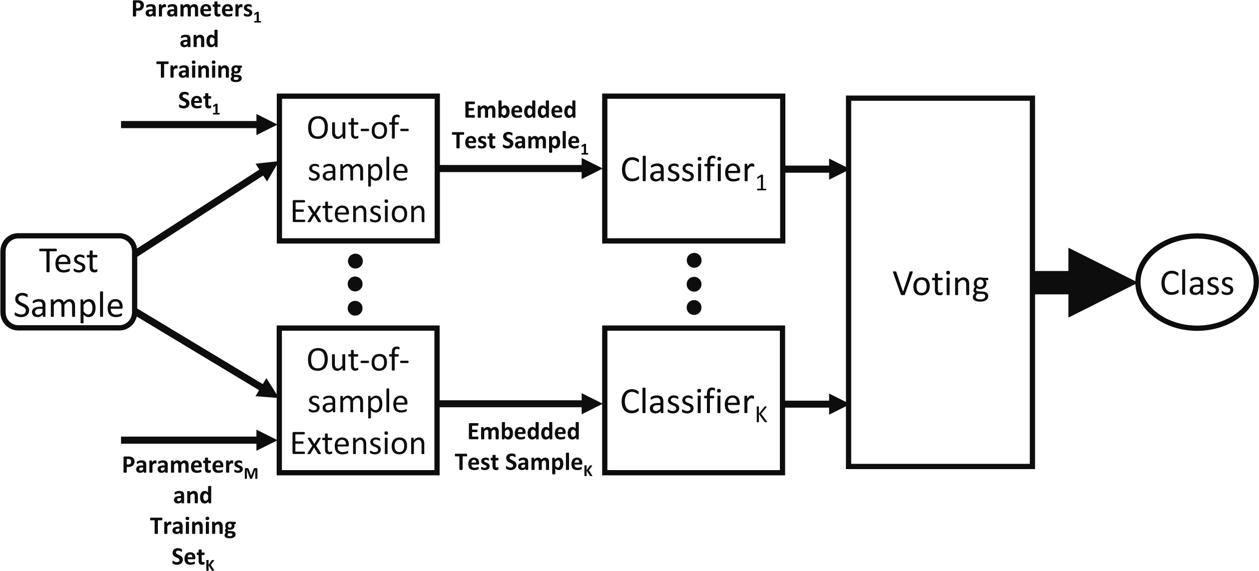

Employing dimensionality reduction to a training set has the following advantages:

•

It can decorrelate the data. For example, Principal Component Analysis transforms a set of data points whose variables may be correlated into a set of linearly uncorrelated variables.

•

It can reduce noise. For example, the noise reduction capabilities of the DM algorithm are described and demonstrated in Section 3.2.

•

It reduces the computational complexity of the classifier construction and consequently the complexity of the classification.

•

It can alleviate over-fitting by constructing combinations of the variables [45].

These points meet the accuracy and diversity criteria which are required to construct an effective ensemble classifier and thus render dimensionality reduction a technique which is tailored for the construction of ensemble classifiers. Specifically, removing noise from the data contributes to the accuracy of the classifier while diversity is obtained by the various dimension-reduced versions of the data.

In order to classify test samples, they are first embedded into the low-dimensional space of each of the training sets using out-of-sample extension. Next, each ensemble member is applied to its corresponding embedded test sample and the produced results are processed by a voting scheme to derive the result of the ensemble classifier. Specifically, each classification is given as a vector containing the probabilities of each possible label. These vectors are aggregated and the ensemble classification is chosen as the label with the largest probability. Figure 2 depicts the classification process of a test sample.

Incorporating a-priori and domain knowledge is known to boost the classification performance in many cases. The proposed framework is general in the sense that it does not require neither a-priori knowledge of the datasets nor their domains. Nevertheless, it allows the incorporation of a-priori knowledge – for example by preprocessing the dataset – provided the resultant dataset is numeric.

3. Diffusion maps

The Diffusion Maps (DM) [11] algorithm embeds data into a low-dimensional space where the geometry of the dataset is defined in terms of the connectivity between every pair of points in the ambient space. Namely, the similarity between two points $x$ and $y$ is determined according to the number of paths connecting $x$ and $y$ via points in the dataset. This measure is robust to noise since it takes into account all the paths connecting $x$ and $y$ . The Euclidean distance between $x$ and $y$ in the dimension-reduced space approximates their connectivity in the ambient space.

Formally, let $\Gamma$ be a set of points in $\mathbb{R}^{n}$ as defined in Eq. (1). A weighted undirected graph $G(V,E),$ $|V|=N,\,|E|\ll N^{2}$ is constructed, where each vertex $v\in V$ corresponds to a point in $\Gamma.$ The weights of the edges are chosen according to a weight function $w_{\varepsilon}\left(x,y\right)$ which measures the similarities between every pair of points where the parameter $\varepsilon$ defines a local neighborhood for each point. The weight function is defined by a kernel function obeying the following properties:

Symmetry:
$\forall x_{i},x_{j}\in\Gamma,\,\,w_{\varepsilon}\left(x_{i},x_{j}\right)=w_{% \varepsilon}\left(x_{j},x_{i}\right)$
Non-negativity:
$\forall x_{i},x_{j}\in\Gamma,\,\,w_{\varepsilon}\left(x_{i},x_{j}\right)\geqslant 0$
Positive semi-definite:
For every real-valued bounded function $f$ defined on $\Gamma$ ,

$\sum_{x_{i},x_{j}\in\Gamma}w_{\varepsilon}(x_{i},x_{j})f(x_{i})f(x_{j})% \geqslant 0.$
Fast decay:
$w_{\varepsilon}\left(x_{i},x_{j}\right)\rightarrow 0$ when $\left\|x_{i}-x_{j}\right\|\gg\varepsilon$ and $w_{\varepsilon}\left(x_{i},x_{j}\right)\rightarrow 1$ when $\left\|x_{i}-x_{j}\right\|\ll\varepsilon$ . This property facilitates the representation of $w_{\varepsilon}$ by a sparse matrix.

A common choice that meets these criteria is the Gaussian kernel:

$w_{\varepsilon}\left(x_{i},x_{j}\right)=e^{-\frac{\left\|x_{i}-x_{j}\right\|^{% 2}}{2\varepsilon}}.$ (3)

A weight matrix $w_{\varepsilon}$ is used to represent the weights of the edges. Given a graph $G$ , the Graph Laplacian normalization [10] is applied to the weight matrix $w_{\varepsilon}$ and the result is given by $M$ :

$M_{i,j}\triangleq m\left(x_{i},x_{j}\right)=\frac{w_{\varepsilon}\left(x_{i},x% _{j}\right)}{d\left(x_{i}\right)}$ (4)

where $d(x_{i})=\sum_{x_{j}\in\Gamma}w_{\varepsilon}\left(x_{i},x_{j}\right)$ is the degree of $x_{i}$ . This transforms $w_{\varepsilon}$ into a Markov transition matrix corresponding to a random walk through the points in $\Gamma$ . The probability to move from $x_{i}$ to $x_{j}$ in one time step is denoted by $m\left(x_{i},x_{j}\right)$ . These probabilities measure the connectivity of the points within the graph.

The transition matrix $M$ is conjugate to a symmetric matrix $A$ whose elements are given by

$A_{i,j}\triangleq a\left(x_{i},x_{j}\right)=\sqrt{d\left(x_{i}\right)}m\left(x% _{i},x_{j}\right)\frac{1}{\sqrt{d(x_{j})}}.$

Using matrix notation, $A$ is given by $A=D^{\frac{1}{2}}MD^{-\frac{1}{2}},$ where $D$ is a diagonal matrix whose values are given by $d\left(x_{i}\right)$ . The matrix $A$ has $n$ real eigenvalues $\left\{\lambda_{l}\right\}_{l=0}^{n-1}$ where $0\leqslant\lambda_{l}\leqslant 1,$ and a set of orthonormal eigenvectors $\left\{v_{l}\right\}_{l=1}^{N-1}$ in $\mathbb{R}^{n}$ . Thus, $A$ has the following spectral decomposition:

$a\left(x_{i},x_{j}\right)=\sum_{k\geqslant 0}\lambda_{k}v_{l}\left(i\right)v_{% l}\left(j\right).$ (5)

where $v_{l}\left(i\right)$ and $v_{l}\left(j\right)$ denote the i- $t h$ and $j$ -th coordinates of the eigenvector $v_{l}$ , respectively. Since $M$ is conjugate to $A$ , the eigenvalues of both matrices are identical. In addition, if $\left\{\phi_{l}\right\}$ and $\left\{\psi_{l}\right\}$ are the left and right eigenvectors of $M$ , respectively, then the following equalities hold:

$\phi_{l}=D^{\frac{1}{2}}v_{l},\;\;\psi_{l}=D^{-\frac{1}{2}}v_{l}.$ (6)

From the orthonormality of $\left\{v_{i}\right\}$ and Eq. (6) it follows that $\left\{\phi_{l}\right\}$ and $\left\{\psi_{l}\right\}$ are bi-orthonormal i.e. $\langle\phi_{m},\psi_{l}\rangle=\delta_{ml}$ where $\delta_{ml}=1$ when $m=l$ and $\delta_{ml}=0$ , otherwise. Combing(Eqs 5) and (6) together with the bi-orthogonality of $\left\{\phi_{l}\right\}$ and $\left\{\psi_{l}\right\}$ leads to the following eigen-decomposition of the transition matrix $M$

$m(x_{i},x_{j})=\sum_{l\geqslant 0}\lambda_{l}\psi_{l}\left(i\right)\phi_{l}% \left(j\right).$ (7)

When the spectrum decays rapidly (provided $\varepsilon$ is appropriately chosen – see Section 3.1), only a few terms are required to achieve a given accuracy in the sum. Namely,

$m\left(x_{i},x_{j}\right)\backsimeq\sum_{l=0}^{n\left(p\right)}\lambda_{l}\psi% _{l}\left(i\right)\phi_{l}\left(j\right)$

where $n\left(p\right)$ is the number of terms which are required to achieve a given precision $p$ .

We recall the diffusion distance between two data points $x_{i}$ and $x_{j}$ as it was defined in [11]:

$D^{2}\left(x_{i},x_{j}\right)=\sum_{z\in\Gamma}\frac{\left(m\left(x_{i},z% \right)-m\left(z,x_{j}\right)\right)^{2}}{\phi_{0}\left(z\right)}.$ (8)

This distance reflects the geometry of the dataset and it depends on the number of paths connecting $x$ and $y$ . Substituting Eq. (7) in Eq. (8) together with the bi-orthogonality property allows to express the diffusion distance using the right eigenvectors of the transition matrix $M$ :

$D^{2}\left(x_{i},x_{j}\right)=\sum_{l\geqslant 1}\lambda_{l}^{2}\left(\psi_{l}% \left(i\right)-\psi_{l}\left(j\right)\right)^{2}.$ (9)

Thus, the family of Diffusion Maps $\left\{\Psi(x)\right\}$ which is defined by

$\Psi(x)=\left(\lambda_{1}\psi_{1}(x),\lambda_{2}\psi_{2}(x),\lambda_{3}\psi_{3% }(x),\ldots\right)$ (10)

embeds the dataset into a Euclidean space. In the new coordinates of Eq. (10), the Euclideandistance between two points in the embedding space is equal to the diffusion distance between their corresponding two high dimensional points as defined by the random walk. Moreover, this facilitates the embedding of the original points into a low-dimensional Euclidean space $\mathbb{R}^{q}$ by:

$\Xi_{t}:x_{i}\rightarrow\left(\lambda_{2}^{t}\psi_{2}\left(x_{i}\right),% \lambda_{3}^{t}\psi_{3}\left(x_{i}\right),\dots,\lambda_{q+1}^{t}\psi_{q+1}% \left(x_{i}\right)\right).$ (11)

which also endows coordinates on the set $\Gamma$ . Since $\lambda_{1}=1$ and $\psi_{1}(x)$ is constant, the embedding uses $\lambda_{2},\ldots,\lambda_{q+1}$ . Essentially, $q\ll n$ due to the fast decay of the eigenvalues of $M$ . Furthermore, $q$ depends only on the dimensionality of the data as captured by the random walk and not on the original dimensionality of the data. Diffusion maps have been successfully applied for acoustic detection of moving vehicles [53] and fusion of data and multicue data matching [37].
3.1 Choosing $\varepsilon$

The Gaussian kernel Eq. (3) produces a similarity value on the scale of $[0,1]$ . The choice of $\varepsilon$ is critical to achieve the optimal performance by the DM algorithm since it defines the size of the local neighborhood of each point. On one hand, a large $\varepsilon$ produces a coarse analysis of the data as the neighborhood of each point will contain a large number of points. For example, if we choose

$\varepsilon=\frac{\alpha}{2}\cdot\max_{x_{i},x_{j}\in\Gamma}\left\|x_{i}-x_{j}% \right\|^{2},$

where $\alpha\gg\max_{x_{i},x_{j}\in\Gamma}\left\|x_{i}-x_{j}\right\|^{2}$ , then all similarities will be close to 1 since

$w_{\varepsilon}\left(x_{i},x_{j}\right)=e^{-\frac{\left\|x_{i}-x_{j}\right\|^{% 2}}{2\varepsilon}}\geqslant e^{-\frac{1}{\alpha}}\sim 1.$

This means that all the points in the dataset will be included in the neighborhoods of the rest of the points. On the other hand, a small $\varepsilon$ might produce many neighborhoods that contain only a single point. For example, if we choose $\varepsilon=\frac{\alpha}{2}\cdot\min_{x_{i},x_{j}\in\Gamma}\left\|x_{i}-x_{j}% \right\|^{2}$ , where $\alpha\ll\min_{x_{i},x_{j}\in\Gamma}\left\|x_{i}-x_{j}\right\|^{2}$ , then all similarities will be close to 0 because

$w_{\varepsilon}\left(x_{i},x_{j}\right)=e^{-\frac{\left\|x_{i}-x_{j}\right\|^{% 2}}{2\varepsilon}}\leqslant e^{-\frac{1}{\alpha}}\sim 0.$

In this case no points will be included in the neighborhood of the rest of the points in the dataset. The best choice, which is vital for the discovery of the dataset structure, lies between these two extremes. Finding the optimal value of $\varepsilon$ is a difficult task. Thus, the ensemble classifier which is based on the Diffusion Maps algorithm will construct different versions of the training set using different values of $\varepsilon$ which will be chosen between the smallest and largest similarities.

3.2 Noise reduction

The DM algorithm can reduce noise under some constraints. Suppose each point is perturbed by some additive noise function $\nu:\Gamma\rightarrow\mathbb{R}^{n}$ such that each point in $\Gamma$ can be written as $x+\nu(x)$ . If the weight function $w_{\varepsilon}$ is smooth, e.g. a Gausssian, then the effect of the noise can be linearized such that

$w_{\varepsilon}\left(x_{i}+\nu\left(x_{i}\right),x_{j}+\nu\left(x_{j}\right)% \right)=w_{\varepsilon}\left(x_{i},x_{j}\right)+O\left(\frac{\left\|\nu\right% \|}{\sqrt{\varepsilon}}\right).$

Consequently, the noise effect on the Markov transition matrix $M$ Eq. (4) is of the same order i.e.

$\hat{m}\left(x_{i},x_{j}\right)=m\left(x_{i},x_{j}\right)+O\left(\frac{\left\|% \nu\right\|}{\sqrt{\varepsilon}}\right).$

where $\hat{m}$ is the perturbed version of $m$ .

Let $\hat{\lambda}_{k}$ be the $k$ -th eigenvalue of the matrix $M$ Eq. (4) where the eigenvalues $\{\hat{\lambda}_{k}\}$ are ordered in descending order. Weyl’s inequality can be used to find the effect of the noise on the eigenvalues and eigenvectors:

$\sup_{k}|\hat{\lambda}_{k}-\lambda_{k}|\leqslant\|\hat{M}-M\|.$

Thus, the influence of the noise on the embedding is limited as long as the noise is smaller than $\sqrt{\varepsilon}$ . We demonstrate the noise reduction capabilities of the DM algorithm in Fig. 3. The DM algorithm is applied to a paraboloid (Fig. 3 left) to which Gaussian noise was added. It can be seen that DM successfully discovered the two parameters that constitute the parabolid (Fig. 3 right) while reducing the noise.

Figure 3.

Noise reduction example of the DM algorithm.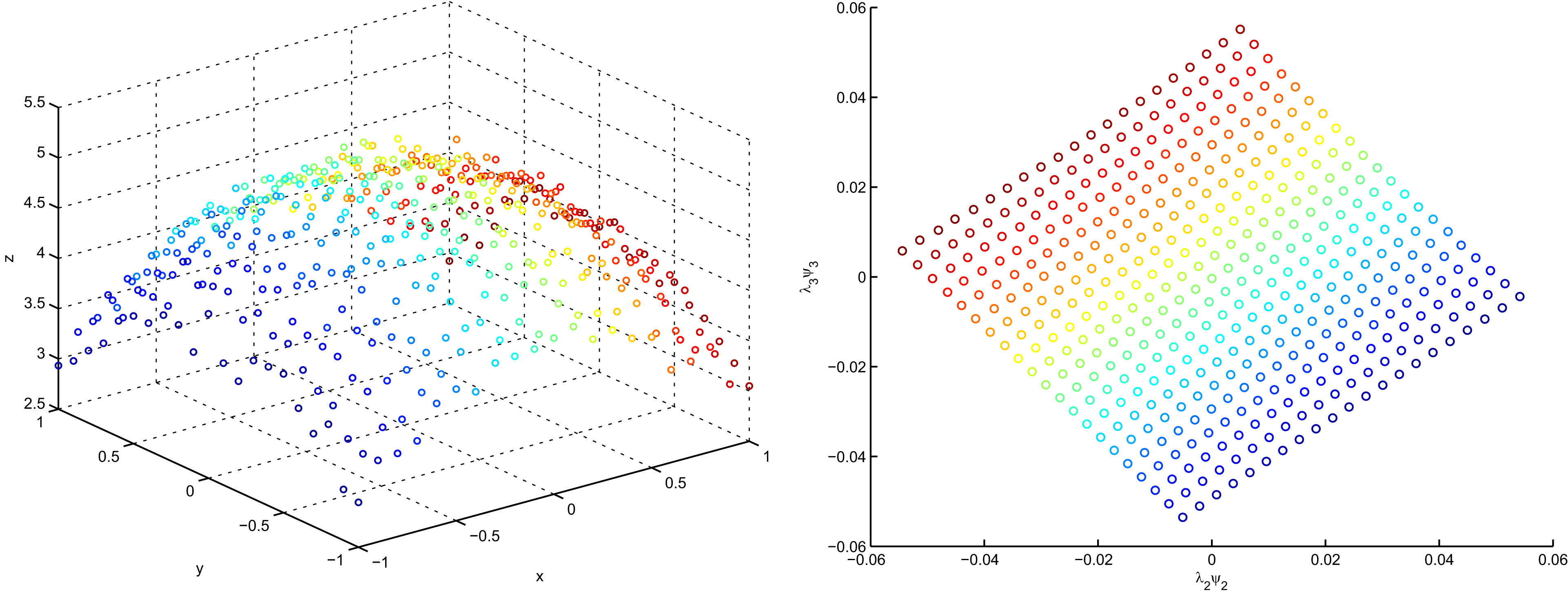

3.3 The Nyström out-of-sample extension

The Nyström extension [44] is an extrapolation method that facilitates the extension of any function $f:\Gamma\rightarrow\mathbb{R}$ to a set of new points which are added to $\Gamma$ . Such extensions are required in on-line processes in which new samples arrive and a function $f$ that is defined on $\Gamma$ needs to be extrapolated to include the new points. These settings exactly fit the settings of the proposed approach since the test samples are given after the dimensionality of the training set was reduced. Specifically, the Nyström extension is used to embed a new point into the dimension-reduced space where every coordinate of the low-dimensional embedding constitutes a function that needs to be extended.

We describe the Nyström extension scheme for the Gaussian kernel that is used by the Diffusion Maps algorithm. Let $\Gamma$ be a set of points in $\mathbb{R}^{n}$ and $\Psi$ be its embedding (Eq. (10)). Let $\bar{\Gamma}$ be a set in $\mathbb{R}^{n}$ such that $\Gamma\subset\bar{\Gamma}$ . The Nyström extension scheme extends $\Psi$ onto the dataset $\bar{\Gamma}$ . Recall that the eigenvectors and eigenvalues form the dimension-reduced coordinates of $\Gamma$ (Eq. (11)). The eigenvectors and eigenvalues of a Gaussian kernel with width $\varepsilon$ which is used to measure the pairwise similarities in the training set $\Gamma$ are computed according to

$\lambda_{l}\varphi_{l}(x)=\sum_{y\in\Gamma}e^{-\frac{\parallel x-y\parallel^{2% }}{2\varepsilon}}\varphi_{l}\left(y\right),\mbox{ $x\in\Gamma.$}$ (12)

If $\lambda_{l}\neq 0$ for every $l$ , the eigenvectors in Eq. (12) can be extended to any $x\in\mathbb{R}^{n}$ by

$\bar{\varphi}_{l}(x)=\frac{1}{\lambda_{l}}\sum_{y\in\Gamma}e^{-\frac{\parallel x% -y\parallel^{2}}{2\varepsilon}}\varphi_{l}\left(y\right),\mbox{ $x\in\mathbb{R% }^{n}$.}$ (13)

Let $f$ be a function on the training set $\Gamma$ and let $x\notin\Gamma$ be a new point. In the Diffusion Maps setting, we are interested in approximating

$\Psi(x)=\left(\lambda_{2}\psi_{2}(x),\lambda_{3}\psi_{3}(x),\ldots,\lambda_{q+% 1}\psi_{q+1}(x)\right).$

The eigenfunctions $\left\{\varphi_{l}\right\}$ are the outcome of the spectral decomposition of a symmetric positive matrix. Thus, they form an orthonormal basis in $\mathbb{R}^{N}$ where $N$ is the number of points in $\Gamma$ . Consequently, any function $f$ can be written as a linear combination of this basis:

$f(x)=\sum_{l}\langle\varphi_{l},f\rangle\varphi_{l}(x),\mbox{ $x\in\Gamma.$}$

Using the Nyström extension, as given in Eq. (13), $f$ can be defined for any point in $\mathbb{R}^{n}$ by

$\bar{f}(x)=\sum_{l}\langle\varphi_{l},f\rangle\bar{\varphi_{l}}(x),\mbox{ $x% \in\mathbb{R}^{n}.$}$ (14)

The above extension facilitates the decomposition of every diffusion coordinate $\psi_{i}$ as $\psi_{i}(x)=\sum_{l}\langle\varphi_{l},\psi_{i}\rangle\varphi_{l}(x),\mbox{ $x% \in\Gamma$}$ . In addition, the embedding of a new point $\bar{x}\in\bar{\Gamma}\backslash\Gamma$ can be evaluated in the embedding coordinate system by $\bar{\psi_{i}}\left(\bar{x}\right)=\sum_{l}\langle\varphi_{l},\psi_{i}\rangle% \bar{\varphi_{l}}\left(\bar{x}\right)$ .

Note that the scheme is ill conditioned since $\lambda_{l}\longrightarrow 0$ as $l\longrightarrow\infty$ . This can be solved by cutting-off the sum in Eq. (14) and keeping only the eigenvalues (and their corresponding eigenfunctions) that satisfy $\lambda_{l}\geqslant\delta\lambda_{0}$ (where $0<\delta\leqslant 1$ and the eigenvalues are given in descending order of magnitude):

$\bar{f}(x)=\sum_{\lambda_{l}\geqslant\delta\lambda_{0}}\langle\varphi_{l},f% \rangle\bar{\varphi_{l}}(x),\mbox{ $x\in\mathbb{R}^{n}$.}$ (15)

The result is an extension scheme with a condition number $\delta$ . In this new scheme, $f$ and $\bar{f}$ do not coincide on $\Gamma$ but they are relatively close. The value of $\varepsilon$ controls this error. Thus, choosing $\varepsilon$ carefully may improve the accuracy of the extension.

3.4 Ensemble via diffusion maps

Let $\Gamma$ be a training set as described in Eq. (1). Every dimension-reduced version of $\Gamma$ is constructed by applying the Diffusion Maps algorithm to $\Gamma$ where the parameter $\varepsilon$ is randomly chosen from the set of all pairwise Euclidean distances between the points in $\Gamma$ i.e. from $\left\{\parallel x-y\parallel\right\}_{x,y\in\Gamma}$ . The dimension of the reduced space is fixed for all the ensemble members at a given percentage of the ambient space dimension. We denote by $\widetilde{\Gamma}\left(\varepsilon_{i}\right)\subseteq\mathbb{R}^{q}$ the training set that is obtained from the application of the diffusion maps algorithm to $\Gamma$ using the randomly chosen value $\varepsilon_{i}$ where $i=1,\ldots,K$ and $K$ is the number of ensemble members. The ensemble members are constructed by applying a given induction algorithm to each training set $\widetilde{\Gamma}\left(\varepsilon_{i}\right)$ . In order to classify a new sample, it is first embedded into the dimension-reduced space $\mathbb{R}^{q}$ of each classifier using the Nyström extension (Section 3.3). Then, every ensemble member classifies the new sample and the voting scheme which is described in Section 2 is used to produce the ensemble classification. Note that in order for the Nyström extension to work, each ensemble member must store the eigenvectors and eigenvalues which were produced by the Diffusion Maps algorithm.

4. Random projections

The Random projections algorithm implements the Johnson and Lindenstrauss lemma [33] (see Section 1.2). In order to reduce the dimensionality of a given training set $\Gamma$ , a set of random vectors $\Upsilon=\left\{\rho_{i}\right\}_{i=1}^{n}$ is generated where $\rho_{i}\in\mathbb{R}^{q}$ are column vectors and $\left\|\rho_{i}\right\|_{l_{2}}=1$ .Two common ways to choose the entries of the vectors $\left\{\rho_{i}\right\}_{i=1}^{n}$ are:

1.
From a uniform (or normal) distribution over the $q$ dimensional unit sphere.
2.
From a Bernoulli $+1/-1$ distribution. In this case, the vectors are normalized so that $\left\|\rho_{i}\right\|_{l_{2}}=1$ for $i=1,\ldots,n$ .

Next, the vectors in $\Upsilon$ are used to form the columns of a $q\times n$ matrix

$R=\left(\rho_{1}|\rho_{2}|\ldots|\rho_{n}\right).$ (16)

The embedding $\widetilde{x}_{i}$ of $x_{i}$ is obtained by

$\widetilde{x}_{i}=R\cdot x_{i}$

Random projections are well suited for the construction of ensembles of classifiers since the randomization meets the diversity criterion (Section 1.1) while the bounded distortion rate provides the accuracy.

Random projections have been successfully employed for dimensionality reduction in [21] as part of an ensemble algorithm for clustering. An Expectation Maximization (of Gaussian mixtures) clustering algorithm was applied to the dimension-reduced data. The ensemble algorithm achieved results that were superior to those obtained by: (a) a single run of random projection/clustering; and (b) a similar scheme which used PCA to reduce the dimensionality of the data.
4.1 Out-of-sample extension

In order to embed a new sample $y$ into the dimension-reduced space $\mathbb{R}^{q}$ of the i-th ensemble member, the sample is simply projected onto the random matrix $R$ that was used to reduce the dimensionality of the member’s training set. The embedding of $y$ is given by $\tilde{y}$ $=$ $R\cdot y$ . Accordingly, each random matrix needs to be stored as part of its corresponding ensemble member in order to allow out-of-sample extension.

4.2 Ensemble via random projections

In order to construct the dimension-reduced versions of the training set, $K$ random matrices $\left\{R_{i}\right\}_{i=1}^{K}$ are constructed (recall that $K$ is the number of ensemble members). The training set is projected onto each random matrix $R_{i}$ and the dataset which is produced by each projection is denoted by $\Gamma\left(R_{i}\right)$ . The ensemble members are constructed by applying a given inducer to each of the dimension-reduced datasets in $\left\{\Gamma\left(R_{i}\right)\right\}_{i=1}^{K}$ .

A new sample is classified by first embedding it into the dimension-reduced space $\mathbb{R}^{q}$ of every classifier using the scheme in Section 4.1. Then, each ensemble member classifies the new sample and the voting scheme from Section 2 is used to determine the classification by the ensemble.

5. Random subspaces

The Random subspaces algorithm reduces the dimensionality of a given training set $\Gamma$ by projecting the vectors onto a random subset of attributes. Formally, let $\left\{i_{k}\right\}_{k=1}^{q}$ be a randomly chosen subset of attributes. The embedding $\widetilde{x}$ of $x=\left(x_{1},\ldots,x_{n}\right)$ is obtained by $\widetilde{x}=\left(x_{i_{1}},\ldots,x_{i_{q}}\right)$ . Accordingly, each random set of attributes needs to be stored as part of its corresponding ensemble member.

This method is a special case of the random projections dimensionality reduction algorithm described in Section 4 where the rows (and column) of the matrix $R$ in Eq. (16) are unique indicator vectors.

Random subspaces have been used to construct decision forests [28] – an ensemble of tree classifiers – and also to construct ensemble regressors [50]. Ensemble regressors employ a multivariate function instead of a voting scheme to combine the individual results of the ensemble members. The training sets that are constructed by the Random subspaces method are dimension-reduced versions of the original dataset and therefore this method is investigated in our experiments. This method combined with support vector machines has been successfully applied to relevance feedback in image retrieval [60].

5.1 Out-of-sample extension

In order to embed a new sample $y$ into the dimension-reduced space $\mathbb{R}^{q}$ of the i-th ensemble member, the sample is simply projected onto $\left\{i_{k}\right\}_{k=1}^{q}$ – the member’s subset of attributes. The embedding of $y=\left(y,\ldots,y_{n}\right)$ is given by $\tilde{y}=\left(y_{i_{1}},\ldots,y_{i_{q}}\right)$ .

5.2 Ensemble via random subspaces

In order to construct the dimension-reduced versions of the training set, $K$ subsets of features are randomly chosen. The training set is projected onto each attribute subset and the ensemble members are constructed by applying a given inducer to each of the dimension-reduced datasets.

A new sample is classified by first embedding it into the dimension-reduced space $\mathbb{R}^{q}$ of every classifier using the scheme in Section 5.1. Then, each ensemble member classifies the new sample and the voting scheme from Section 2 is used to determine the ensemble’s classification.

6. Experimental results

In order to evaluate the proposed approach, we used the WEKA framework [25]. We tested our approach on 17 datasets from the UCI repository [39] which contains benchmark datasets that are commonly used to evaluate machine learning algorithms. None of the datasets contain missing values. No a-priori knowledge of the datasets and their domains was used in the experiments. The list of datasets and their properties are summarized in Table 1.

Table 1
Properties of the benchmark datasets used for the evaluation

Dataset name	Instances	Features	Labels	Noise content	Reference
Musk1	476	166	2	None	[16]
Musk2	6598	166	2	None	[31]
Pima-diabetes	768	8	2	None	[59]
Ecoli	335	7	8	None	[29]
Glass	214	9	7	N/A	[20]
Hill Valley with noise	1212	100	2	Yes	[39]
Hill Valley without noise	1212	100	2	None	[39]
Ionosphere	351	34	2	None	[58]
Iris	150	4	3	None	[19]
Isolet	7797	617	26	Recording background	[13]
				and closure noise
Letter	20000	16	26	Yes – random distortion	[23]
Madelon	2000	500	2	480 distractor features	[24]
Multiple features	2000	649	10	None	[63]
Sat	6435	36	7	None	[39]
Waveform with noise	5000	40	3	19 attributes are all noise	[7]
				with mean 0 and variance 1
Waveform without noise	5000	21	3	None	[7]
Yeast	1484	8	10	None	[29]

6.1 Experiment configuration

In order to reduce the dimensionality of a given training set, one of two schemes was employed depending on the dimensionality reduction algorithm at hand. The first scheme was used for the Random Projection and the Random Subspaces algorithms and it applied the dimensionality reduction algorithm to the dataset without any pre-processing of the dataset. However, due to the space and time complexity of the Diffusion Maps algorithm, which is quadratic in the size of the dataset, a different scheme was used. First, a random value $\varepsilon\in\left\{\parallel x-y\parallel\right\}_{x,y\in\Gamma}$ was selected. Next, a random sample of $600$ unique data items was drawn (this size was set according to time and memory limitations). The Diffusion Maps algorithm was then applied to the sample which produced a dimension-reduced training set. This set was then extended using the Nyström extension to include the training samples which were not part of the sample. These steps are summarized in Algorithm 1.

Algorithm 1
Steps for constructing the training set of a single ensemble member using the Diffusion Maps algorithm.

Input: Dataset $\Gamma$ , target dimension $q$

Output: A dimension reduced training set $\widetilde{\widetilde{\Gamma}}$ .

1. 1.
Select a random value $\varepsilon\in\left\{\parallel x-y\parallel\right\}_{x,y\in\Gamma}$
2.
Select a random sample $\bar{\Gamma}$ of $600$ unique elements from $\Gamma$ .
3.
Apply the Diffusion Maps algorithm to $\bar{\Gamma}$ resulting in $\widetilde{\Gamma}$
4.
Extend $\widetilde{\Gamma}$ to include the points in $\Gamma\backslash\bar{\Gamma}$ using the Nyström extension – resulting in $\widetilde{\widetilde{\Gamma}}$ .

All ensemble algorithms were tested using the following inducers: (a) nearest-neighbor (WEKA’s B1 inducer); (b) decision tree (WEKA’s J48 inducer); and (c) Naïve Bayes. The ensembles were composed of ten classifiers (the information theoretic problem of choosing the optimal size of an ensemble is out of the scope of this paper. This problem is discussed, for example, in [35]). The dimension-reduced space was set to half of the original dimension of the data. Ten-fold cross validation was used to evaluate each ensemble’s performance on each of the datasets.

The constructed ensemble classifiers were compared with: a non-ensemble classifier which applied the induction algorithm to the dataset without dimensionality reduction (we refer to this classifier as the plain classifier). The constructed ensemble classifiers were also compared with the Bagging [6], AdaBoost [22] and Rotation Forest [47] ensemble algorithms. In order to see whether the Diffusion Maps ensemble classifier can be further improved as part of a multi-strategy ensemble (Section 1.1), we constructed an ensemble classifier whose members applied the AdaBoost algorithm to their Diffusion Maps dimension-reduced training sets.

We used the default values of the parameters of the WEKA built-in ensemble classifiers in all the experiments. For the sake of simplicity, in the following we refer to the ensemble classifiers which use the Diffusion Maps and Random Projections dimensionality algorithms as the DME and RPE classifiers, respectively. The ensemble classifier which is based on the random subspaces dimensionality reduction algorithm is referred to as the RSE classifier.
6.2 Results

Tables 2–4 describe the results obtained by the decision tree, nearest-neighbor and Naïve Bayes inducers, respectively. In each of the tables, the first column specifies the name of the tested dataset and the second column contains the results of the plain classifier. The second to last row contains the average improvement percentage of each algorithm compared to the plain classifier. We calculate the average rank of each inducer across all datasets in the following manner: for each of the datasets, the algorithms are ranked according to the accuracy that they achieved. The average rank of a given inducer is obtained by averaging its obtained ranks over all the datasets. The average rank is given in the last row of each table.

The results of the experimental study indicate that dimensionality reduction is a promising approach for the construction of ensembles of classifiers. In 113 out of 204 cases the dimensionality reduction ensembles outperformed the plain algorithm with the following distribution: RPE (33 cases out of 113), DM $+$ AdaBoost (30 cases), RSE (27 cases) and DM (23 cases).

Ranking all the algorithms according to the average accuracy improvement percentage produces the following order: Rotation Forest (6.4%), Random projection (4%), DM $+$ AdaBoost (2.1%), Bagging (1.5%), AdaBoost (1%), DM (0.7%) and Random subspaces ( $-$ 6.7%). Note that the RSE algorithm achieved an average decrease of 6.7% in accuracy. A closer look reveals that this was caused by a particularly bad performance when the Naïve Bayes inducer was used (26% average decrease in accuracy). In contrast, improvement averages of 1.7% and 4.4% were achieved when the RSE algorithm used the nearest-neighbors and J48 inducers, respectively. This may be due to datasets whose features are not independent – a situation which does not conform with the basic assumption of the Naïve Bayes inducer. For example, the Isolet dataset is composed of acoustic recordings that are decomposed to overlapping segments where features of each segment constitute an instance in the dataset. In these settings, the features are not independent. Since the other algorithms, including the plain one, achieve much better results when applied to this dataset, we can assume that because the RSE algorithm chooses a random subset of features, the chance of obtaining independent features is lower compared to when all features are selected. Moreover, given the voting scheme in Section 2, ensemble members which produce wrong

Table 2
Results of the ensemble classifiers based on the nearest-neighbor inducer (WEKA’s IB1)

Dataset	Plain NN	RPE	RSE	Bagging	DME	DME $+$ AdaBoost	AdaBoost	Rotation forest
Musk1	84.89 $\pm$ 4.56	86.15 $\pm$ 2.94	86.98 $\pm$ 4.18	86.77 $\pm$ 4.32	84.46 $\pm$ 4.31	84.87 $\pm$ 4.52	87.42 $\pm$ 4.24	84.88 $\pm$ 3.92
Musk2	95.80 $\pm$ 0.34	95.62 $\pm$ 0.38	96.04 $\pm$ 0.33	95.89 $\pm$ 0.31	95.39 $\pm$ 0.39	95.94 $\pm$ 0.49	96.03 $\pm$ 0.35	95.60 $\pm$ 0.62
pima-diabetes	70.17 $\pm$ 4.69	72.14 $\pm$ 4.03	70.83 $\pm$ 3.58	70.44 $\pm$ 3.89	66.79 $\pm$ 4.58	66.40 $\pm$ 4.82	67.30 $\pm$ 5.61	70.04 $\pm$ 4.17
Ecoli	80.37 $\pm$ 6.38	83.02 $\pm$ 3.52	83.05 $\pm$ 6.94	80.96 $\pm$ 5.43	77.37 $\pm$ 6.63	76.48 $\pm$ 8.23	78.87 $\pm$ 7.19	81.56 $\pm$ 4.97
Glass	70.52 $\pm$ 8.94	76.67 $\pm$ 7.22	77.58 $\pm$ 6.55	70.52 $\pm$ 8.94	72.88 $\pm$ 8.51	71.97 $\pm$ 7.25	70.95 $\pm$ 8.12	70.04 $\pm$ 8.24
Hill Valley with noise	59.83 $\pm$ 5.48	68.74 $\pm$ 3.58	59.75 $\pm$ 4.29	59.74 $\pm$ 4.77	50.49 $\pm$ 4.75	50.41 $\pm$ 4.49	58.42 $\pm$ 3.80	79.30 $\pm$ 3.60
Hill Valley w/o noise	65.84 $\pm$ 4.31	79.21 $\pm$ 3.19	66.66 $\pm$ 4.48	65.67 $\pm$ 4.26	55.36 $\pm$ 5.60	54.45 $\pm$ 5.18	63.20 $\pm$ 4.28	92.74 $\pm$ 2.10
Ionosphere	86.33 $\pm$ 4.59	90.02 $\pm$ 5.60	90.30 $\pm$ 4.32	86.90 $\pm$ 4.85	92.88 $\pm$ 4.09	93.44 $\pm$ 4.68	87.48 $\pm$ 3.55	86.61 $\pm$ 4.26
Iris	95.33 $\pm$ 5.49	93.33 $\pm$ 8.31	92.00 $\pm$ 10.80	96.00 $\pm$ 4.66	94.00 $\pm$ 5.84	94.00 $\pm$ 5.84	95.33 $\pm$ 5.49	94.00 $\pm$ 5.84
Isolet	89.94 $\pm$ 0.71	90.61 $\pm$ 0.86	90.57 $\pm$ 0.70	89.59 $\pm$ 0.65	91.32 $\pm$ 0.72	91.54 $\pm$ 0.87	89.00 $\pm$ 0.86	89.78 $\pm$ 0.78
Letter	96.00 $\pm$ 0.60	93.64 $\pm$ 0.32	94.08 $\pm$ 0.76	96.00 $\pm$ 0.57	90.58 $\pm$ 0.70	90.50 $\pm$ 0.76	95.10 $\pm$ 0.43	96.25 $\pm$ 0.55
Madelon	54.15 $\pm$ 4.28	68.95 $\pm$ 3.59	55.65 $\pm$ 2.63	54.80 $\pm$ 3.29	65.60 $\pm$ 1.94	65.10 $\pm$ 2.38	54.35 $\pm$ 4.76	55.20 $\pm$ 3.54
Multiple features	97.80 $\pm$ 0.63	95.65 $\pm$ 1.20	97.90 $\pm$ 0.66	97.85 $\pm$ 0.75	95.45 $\pm$ 1.42	95.55 $\pm$ 1.12	97.45 $\pm$ 0.64	97.70 $\pm$ 0.59
Sat	90.21 $\pm$ 1.16	91.34 $\pm$ 0.75	91.47 $\pm$ 0.71	90.37 $\pm$ 1.13	89.74 $\pm$ 0.57	89.40 $\pm$ 0.53	89.01 $\pm$ 1.32	90.82 $\pm$ 1.07
Waveform with noise	73.62 $\pm$ 1.27	80.14 $\pm$ 1.65	78.14 $\pm$ 2.35	73.74 $\pm$ 1.69	81.78 $\pm$ 0.93	80.72 $\pm$ 0.98	70.80 $\pm$ 2.03	73.94 $\pm$ 1.69
Waveform w/o noise	76.90 $\pm$ 2.01	81.22 $\pm$ 0.90	81.22 $\pm$ 1.47	77.14 $\pm$ 1.55	83.92 $\pm$ 1.38	83.12 $\pm$ 1.16	75.08 $\pm$ 1.70	77.72 $\pm$ 1.39
Yeast	52.29 $\pm$ 2.39	55.53 $\pm$ 4.39	49.32 $\pm$ 4.44	52.49 $\pm$ 2.16	48.99 $\pm$ 3.15	48.59 $\pm$ 4.31	51.35 $\pm$ 1.84	53.30 $\pm$ 2.44
Average improvement	–	5.8%	1.7%	0.4%	$-$ 0.2%	$-$ 0.6%	$-$ 1%	4.6%
Average rank	4.97	3.26	3.15	4.35	5.18	5.29	5.44	4.35

RPE is the Random Projection ensemble algorithm; RSE is the Random Subspaces ensemble algorithm; DME is the Diffusion Maps ensemble classifier; DME $+$ AdaBoost is the multi-strategy ensemble classifier which applied AdaBoost to the Diffusion Maps dimension-reduced datasets.

Table 3

Results of the Random Projection ensemble classifier based on the decision-tree inducer (WEKA’s J48)

Dataset	Plain J48	RPE	RSE	Bagging	DME	DME $+$ AdaBoost	AdaBoost	Rotation forest
Musk1	84.90 $\pm$ 6.61	85.31 $\pm$ 6.25	88.45 $\pm$ 8.20	86.56 $\pm$ 6.93	78.60 $\pm$ 7.78	84.89 $\pm$ 5.44	88.46 $\pm$ 6.38	91.60 $\pm$ 3.10
Musk2	96.88 $\pm$ 0.63	96.30 $\pm$ 0.78	98.26 $\pm$ 0.39	97.65 $\pm$ 0.50	96.76 $\pm$ 0.72	97.23 $\pm$ 0.67	98.77 $\pm$ 0.35	98.18 $\pm$ 0.67
pima-diabetes	73.83 $\pm$ 5.66	73.83 $\pm$ 4.86	73.71 $\pm$ 6.04	75.26 $\pm$ 2.96	72.27 $\pm$ 3.11	72.40 $\pm$ 3.68	72.40 $\pm$ 4.86	76.83 $\pm$ 4.80
Ecoli	84.23 $\pm$ 7.51	86.00 $\pm$ 6.20	84.49 $\pm$ 7.28	84.79 $\pm$ 6.11	83.02 $\pm$ 4.10	81.27 $\pm$ 5.74	83.04 $\pm$ 7.37	86.60 $\pm$ 4.30
Glass	65.87 $\pm$ 8.91	72.94 $\pm$ 8.19	76.62 $\pm$ 7.38	75.19 $\pm$ 6.40	65.39 $\pm$ 10.54	68.12 $\pm$ 11.07	79.37 $\pm$ 6.13	74.22 $\pm$ 9.72
Hill Valley with noise	49.67 $\pm$ 0.17	71.28 $\pm$ 4.69	49.67 $\pm$ 0.17	54.62 $\pm$ 3.84	52.39 $\pm$ 3.56	52.39 $\pm$ 5.03	49.67 $\pm$ 0.17	74.51 $\pm$ 2.59
Hill Valley w/o noise	50.49 $\pm$ 0.17	86.38 $\pm$ 3.77	50.49 $\pm$ 0.17	50.99 $\pm$ 1.28	51.23 $\pm$ 4.40	52.39 $\pm$ 3.34	50.49 $\pm$ 0.17	83.83 $\pm$ 3.94
Ionosphere	91.46 $\pm$ 3.27	94.32 $\pm$ 3.51	93.75 $\pm$ 4.39	91.75 $\pm$ 3.89	88.04 $\pm$ 4.80	94.87 $\pm$ 2.62	93.17 $\pm$ 3.57	94.89 $\pm$ 3.45
Iris	96.00 $\pm$ 5.62	95.33 $\pm$ 6.32	94.67 $\pm$ 4.22	94.67 $\pm$ 6.13	92.00 $\pm$ 8.20	90.67 $\pm$ 9.53	93.33 $\pm$ 7.03	96.00 $\pm$ 4.66
Isolet	83.97 $\pm$ 1.65	87.37 $\pm$ 1.46	92.45 $\pm$ 1.14	90.46 $\pm$ 1.29	90.10 $\pm$ 0.62	93.86 $\pm$ 0.43	93.39 $\pm$ 0.67	93.75 $\pm$ 0.76
Letter	87.98 $\pm$ 0.51	88.10 $\pm$ 0.52	93.50 $\pm$ 0.92	92.73 $\pm$ 0.69	89.18 $\pm$ 0.79	91.46 $\pm$ 0.78	95.54 $\pm$ 0.36	95.41 $\pm$ 0.46
Madelon	70.35 $\pm$ 3.78	59.20 $\pm$ 2.57	76.95 $\pm$ 2.69	65.10 $\pm$ 3.73	76.15 $\pm$ 3.43	72.90 $\pm$ 2.27	66.55 $\pm$ 4.09	68.30 $\pm$ 2.98
Multiple features	94.75 $\pm$ 1.92	95.35 $\pm$ 1.31	97.35 $\pm$ 0.88	96.95 $\pm$ 1.07	93.25 $\pm$ 1.64	94.90 $\pm$ 1.73	97.60 $\pm$ 1.13	97.95 $\pm$ 1.04
Sat	85.83 $\pm$ 1.04	90.15 $\pm$ 0.93	91.10 $\pm$ 0.91	90.09 $\pm$ 0.78	91.34 $\pm$ 0.48	91.67 $\pm$ 0.37	90.58 $\pm$ 1.12	90.74 $\pm$ 0.69
Waveform with noise	75.08 $\pm$ 1.33	81.84 $\pm$ 1.43	82.02 $\pm$ 1.50	81.72 $\pm$ 1.43	86.52 $\pm$ 1.78	86.62 $\pm$ 1.76	80.48 $\pm$ 1.91	83.76 $\pm$ 2.07
Waveform w/o noise	75.94 $\pm$ 1.36	82.56 $\pm$ 1.56	82.52 $\pm$ 1.67	81.48 $\pm$ 1.27	86.96 $\pm$ 1.49	86.36 $\pm$ 0.94	81.46 $\pm$ 1.83	84.94 $\pm$ 1.47
Yeast	55.99 $\pm$ 4.77	57.82 $\pm$ 3.28	55.32 $\pm$ 4.06	59.23 $\pm$ 3.25	54.85 $\pm$ 3.94	55.39 $\pm$ 2.94	56.39 $\pm$ 5.08	60.71 $\pm$ 3.82
Average improvement	–	8.5%	4.4%	3.8%	2.2%	3.5%	3.6%	12.2%
Average rank	6.26	4.56	4.03	4.44	5.68	4.41	4.5	2.15

RPE is the Random Projection ensemble algorithm; RSE is the Random Subspaces ensemble algorithm; DME is the Diffusion Maps ensemble classifier; DME $+$ AdaBoost is the multi-strategy ensemble classier which applied AdaBoost to the Diffusion Maps dimension-reduced datasets.

Table 4

Results of the ensemble classifiers based on the Naïve Bayes inducer

Dataset	Plain NB	RPE	RSE	Bagging	DME	DME $+$ AdaBoost	AdaBoost	Rotation forest
Musk1	75.25 $\pm$ 6.89	69.80 $\pm$ 8.98	56.52 $\pm$ 0.70	75.24 $\pm$ 7.11	55.90 $\pm$ 5.09	74.80 $\pm$ 2.88	77.10 $\pm$ 4.50	76.29 $\pm$ 6.76
Musk2	83.86 $\pm$ 2.03	77.36 $\pm$ 2.21	84.59 $\pm$ 0.07	83.71 $\pm$ 1.68	94.13 $\pm$ 0.50	95.74 $\pm$ 0.56	89.51 $\pm$ 1.98	83.98 $\pm$ 1.83
pima-diabetes	76.31 $\pm$ 5.52	70.18 $\pm$ 3.69	71.74 $\pm$ 5.37	76.83 $\pm$ 5.66	72.13 $\pm$ 4.50	71.88 $\pm$ 4.37	76.18 $\pm$ 4.69	74.09 $\pm$ 4.80
Ecoli	85.40 $\pm$ 5.39	86.92 $\pm$ 3.16	80.37 $\pm$ 5.91	87.18 $\pm$ 4.49	84.52 $\pm$ 5.43	84.52 $\pm$ 5.43	85.40 $\pm$ 5.39	86.31 $\pm$ 6.17
Glass	49.48 $\pm$ 9.02	48.07 $\pm$ 11.39	15.61 $\pm$ 10.16	50.82 $\pm$ 10.46	59.29 $\pm$ 11.09	60.24 $\pm$ 10.36	49.48 $\pm$ 9.02	54.16 $\pm$ 8.92
Hill Valley with noise	49.50 $\pm$ 2.94	49.75 $\pm$ 3.40	49.50 $\pm$ 2.94	50.74 $\pm$ 2.88	50.82 $\pm$ 2.93	53.63 $\pm$ 3.77	49.25 $\pm$ 3.39	52.14 $\pm$ 4.21
Hill Valley w/o noise	51.57 $\pm$ 2.64	50.82 $\pm$ 3.00	51.40 $\pm$ 2.52	51.90 $\pm$ 3.16	51.74 $\pm$ 3.25	52.06 $\pm$ 2.53	51.57 $\pm$ 2.61	52.56 $\pm$ 3.51
Ionosphere	82.62 $\pm$ 5.47	83.21 $\pm$ 6.42	67.80 $\pm$ 12.65	81.48 $\pm$ 5.42	92.59 $\pm$ 4.71	93.17 $\pm$ 3.06	92.04 $\pm$ 4.37	84.63 $\pm$ 5.02
Iris	96.00 $\pm$ 4.66	94.67 $\pm$ 4.22	96.67 $\pm$ 3.51	95.33 $\pm$ 5.49	91.33 $\pm$ 6.32	91.33 $\pm$ 6.32	93.33 $\pm$ 7.03	98.00 $\pm$ 3.22
Isolet	85.15 $\pm$ 0.96	89.06 $\pm$ 0.83	3.85 $\pm$ 0.00	85.58 $\pm$ 0.95	91.83 $\pm$ 0.96	92.97 $\pm$ 0.87	85.15 $\pm$ 0.96	90.68 $\pm$ 0.62
Letter	64.11 $\pm$ 0.76	59.27 $\pm$ 2.52	24.82 $\pm$ 8.81	64.18 $\pm$ 0.81	58.31 $\pm$ 0.70	56.90 $\pm$ 1.52	64.11 $\pm$ 0.76	67.51 $\pm$ 0.96
Madelon	58.40 $\pm$ 0.77	59.80 $\pm$ 2.06	50.85 $\pm$ 2.35	58.40 $\pm$ 0.84	55.10 $\pm$ 4.40	60.55 $\pm$ 4.01	53.65 $\pm$ 3.59	58.80 $\pm$ 1.51
Multiple features	95.35 $\pm$ 1.40	83.40 $\pm$ 2.22	10.90 $\pm$ 1.47	95.15 $\pm$ 1.25	89.05 $\pm$ 2.09	96.05 $\pm$ 1.28	96.40 $\pm$ 0.91	95.25 $\pm$ 1.57
Sat	79.58 $\pm$ 1.46	81.90 $\pm$ 1.13	69.82 $\pm$ 4.57	79.61 $\pm$ 1.50	85.63 $\pm$ 1.25	86.23 $\pm$ 1.16	79.58 $\pm$ 1.46	83.36 $\pm$ 1.52
Waveform with noise	80.00 $\pm$ 1.96	80.46 $\pm$ 1.76	72.04 $\pm$ 7.11	80.00 $\pm$ 2.01	84.36 $\pm$ 1.81	84.48 $\pm$ 1.46	80.00 $\pm$ 1.96	81.80 $\pm$ 1.81
Waveform w/o noise	81.02 $\pm$ 1.33	80.48 $\pm$ 2.03	74.48 $\pm$ 5.23	81.06 $\pm$ 1.35	82.94 $\pm$ 1.62	83.44 $\pm$ 1.72	81.02 $\pm$ 1.33	83.26 $\pm$ 1.59
Yeast	57.61 $\pm$ 3.01	55.39 $\pm$ 2.33	38.27 $\pm$ 7.89	57.82 $\pm$ 2.69	53.44 $\pm$ 3.96	53.37 $\pm$ 3.94	57.61 $\pm$ 3.01	55.46 $\pm$ 3.23
Average improvement	–	$-$ 2.3%	$-$ 26.1%	0.4%	0.2%	3.4%	0.6%	2.3%
Average rank	4.71	5.41	7.15	3.97	4.29	3.06	4.59	2.82

RPE is the Random Projection ensemble algorithm; RSE is the Random Subspaces ensemble algorithm; DME is the Diffusion Maps ensemble classifier; DME $+$ AdaBoost is the multi-strategy ensemble classier which applied AdaBoost to the Diffusion Maps dimension-reduced datasets.

classifications with high probabilities damage accurate classifications obtained by other ensemble members. Figure 4 demonstrates how the accuracy decreases as the number of members increases when RSE is paired with the Naïve Bayes inducer. This phenomenon is contrasted in Fig. 5 where the behavior that is expected from the ensemble is observed. Namely, an increase in accuracy when the number of ensemble members is increased when an ensemble different from the RSE is used (e.g. the DME).

In order to compare the 8 algorithms across all inducers and datasets we applied the procedure presented in [15]. The null hypothesis that all methods have the same accuracy could not be rejected by the adjusted Friedman test with a confidence level of 90% (specifically F(7, 350) $=$ 0.79 $<$ 1.73 with $p$ -value $>$ 0.1). Furthermore, the results show there is a dependence between the inducer, dataset and chosen dimensionality reduction algorithm. In the following we investigate the dependence between the latter two for each of the inducers.

Figure 4.

Accuracy of the RSE algorithm using the Naïve Bayes inducer.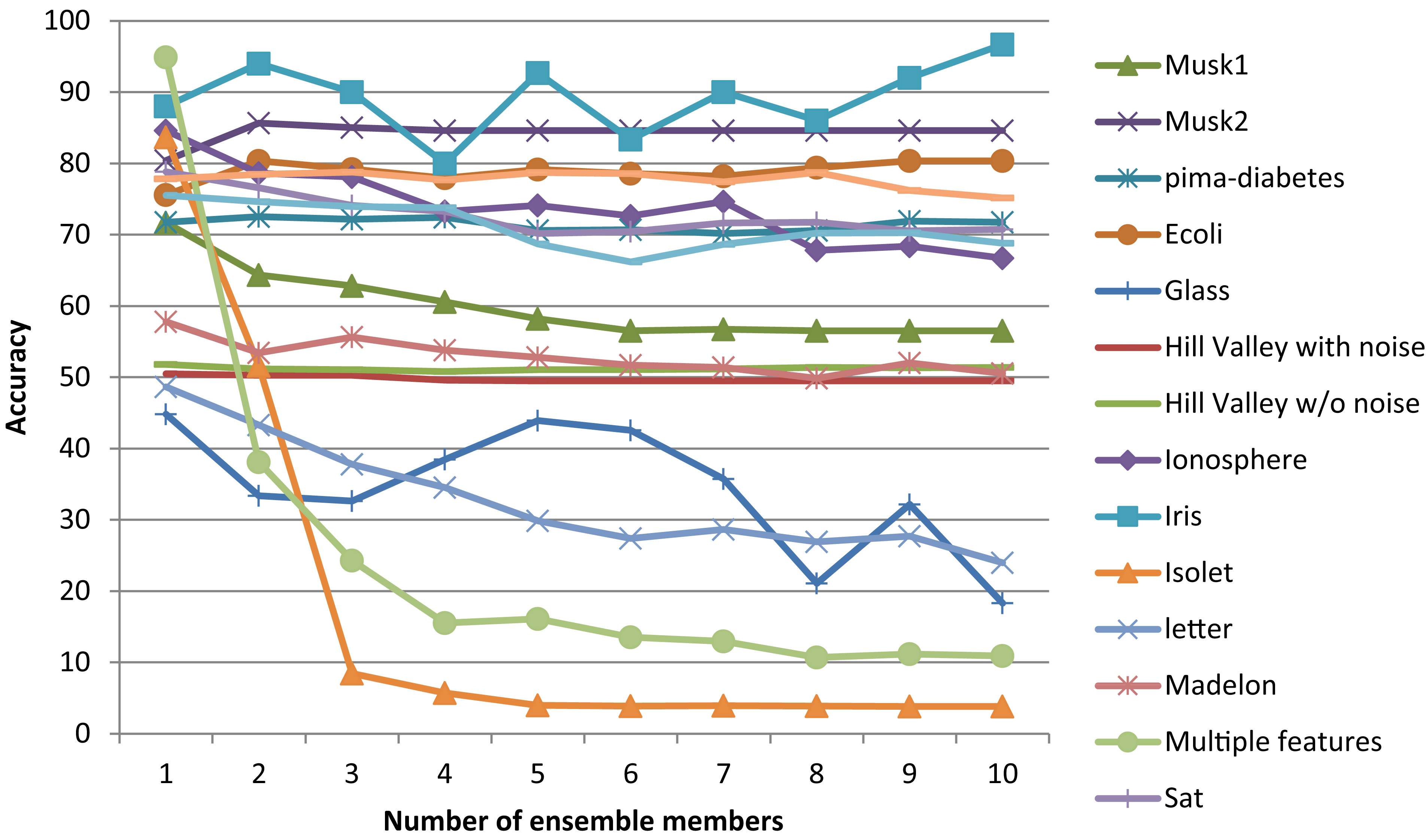

Figure 5.

Accuracy of the DM ensemble using the Naïve Bayes inducer.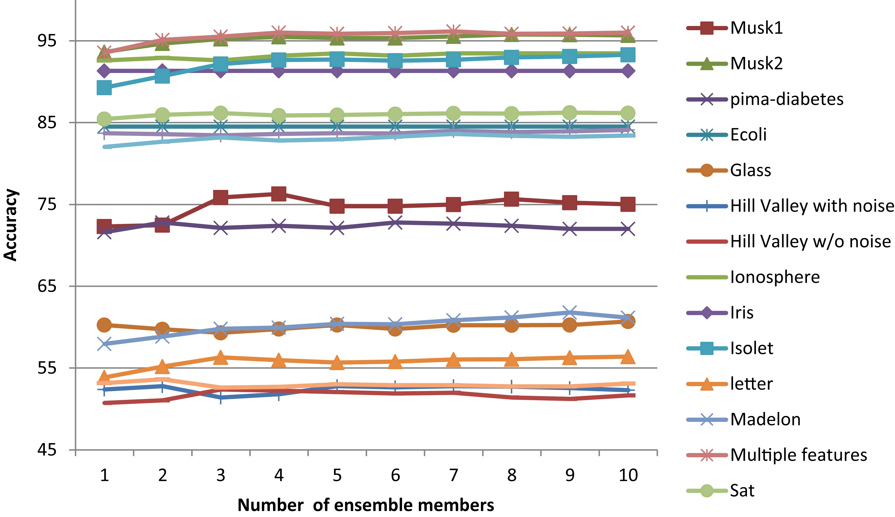

6.2.1 Results for the nearest neighbor inducer (IB1)

In terms of the average improvement, the RPE algorithm is ranked first with an average improvement percentage of 5.8%. We compared the various algorithms according to their average rank following the steps described in [15]. The RSE and RPE achieved the first and second average rank, respectively. They were followed by Bagging ( $3^{\rm rd}$ ) and Rotation Forest ( $4^{\rm th}$ ).

Using the adjusted Friedman test we rejected the null hypothesis that all methods achieve the same classification accuracy with a confidence level of 95% and (7, 112) degrees of freedom (specifically F(7, 112) $=$ 2.47 $>$ 2.09 and $p$ -value $<$ 0.022). Following the rejection of the null hypothesis, we employed the Nemenyi post-hoc test where in the experiment settings two classifiers are significantly different with a confidence level of 95% if their average ranks differ by at least $\textit{CD}=$ 2.55. The null hypothesis that any of the non-plain algorithms has the same accuracy as the plain algorithm could not be rejected at confidence level 95%.

6.2.2 Results for the decision tree inducer (J48)

Inspecting the average improvement, the RPE and RSE algorithms are ranked second and third, respectively, after the Rotation Forest algorithm. Following the procedure presented by Demsar [15], we compared the various algorithms according to their average rank. The RSE and DM $+$ AdaBoost achieved the second and third best average rank, respectively, after the Rotation Forest algorithm.

The null hypothesis that all methods obtain the same classification accuracy was rejected by the adjusted Friedman test with a confidence level of 95% and (7, 112) degrees of freedom (specifically F(7, 112) $=$ 5.17 $>$ 2.09 and $p$ -value $<$ 0.0001). As the null hypothesis was rejected, we employed the Nemenyi post-hoc test ( $\textit{CD}=$ 2.55). Only the Rotation Forest algorithm significantly outperformed the plain and the DM algorithms. The null hypothesis that the RPE, RSE, DM and DM $+$ AdaBoost algorithms have the same accuracy as the plain algorithm could not be rejected at confidence level 90%.

6.2.3 Results for the Naïve Bayes inducer

The DM $+$ AdaBoost algorithm achieved the best average improvement and it is followed by the Rotation Forest algorithm. The DM, RPE and RSE are ranked 5 ${}^{\rm th}$ , 7 ${}^{\rm th}$ and 8 ${}^{\rm th}$ in terms of the average improvement (possible reasons for the RSE algorithm’s low ranking were described in the beginning of this section).

Employing the procedure presented in [15], we compared the algorithms according to their average ranks. The DM $+$ AdaBoost and DM ensembles achieved the second and fourth best average ranks, respectively while the Rotation Forest and Bagging algorithms achieved the first and third places, respectively. The null hypothesis that all methods have the same classification accuracy was rejected by the adjusted Friedman test with a confidence level of 95% and (7, 112) degrees of freedom (specifically F(7, 112) $=$ 7.37 $>$ 2.09 and $p$ -value $<$ 1e-6). Since the null hypothesis was rejected, we employed the Nemenyi post-hoc test. As expected, the RSE was significantly inferior to all other algorithms. Furthermore, the Rotation Forest algorithm was significantly better than the RPE algorithms. However, we could not reject at confidence level 95% the null hypothesis that the RPE, DM, DM $+$ AdaBoost and the plain algorithm have the same accuracy.

When we compare the average accuracy improvement across all the inducers, the RPE and DM $+$ AdaBoost were ranked second and third – improving the plain algorithm by 4% and 2.1%, respectively. The Rotation Forest algorithm is ranked first with 6.4% improvement. Comparing only the proposed ensembles according to their average rank as described in [15] yielded the following ranking: DM $+$ AdaBoost, RPE, RSE, DM. The null hypothesis that the RPE, RSE, DM and DM $+$ AdaBoost algorithms have the same accuracy as the plain algorithm could not be rejected at confidence level 90%. Thus, according to the average accuracy improvement across all the inducers, RPE performs best. However, according to the average rank, DM $+$ AdaBoost performs best.

6.3 Discussion

The results indicate that when a dimensionality reduction algorithm is coupled with an appropriate inducer, an effective ensemble can be constructed. For example, the RPE algorithm achieves the best average improvements when it is paired with the nearest-neighbor and the decision tree inducers. However, when it is used with the Naïve Bayes inducer, it fails to improve the plain algorithm. On the other hand, the DM $+$ AdaBoost ensemble obtains the best average improvement when it is used with the Naïve Bayes inducer (better than the current state-of-the-art Rotation Forest ensemble algorithm) and it is less accurate when coupled with the decision tree and nearest-neighbor inducers.

Furthermore, using dimensionality reduction as part of a multi-strategy ensemble classifier improved in most cases the results of the ensemble classifiers which employed only one of the strategies. Specifically, the DM $+$ AdaBoost algorithm achieved higher average ranks compared to the DM and AdaBoost algorithms when the J48 and Naïve Bayes inducers were used. When the nearest-neighbor inducer was used, the DM $+$ AdaBoost algorithm was ranked after the DM algorithm and before the AdaBoost ensemble which was last.

7. Conclusion and future work

In this paper we presented dimensionality reduction as a general framework for the construction of ensemble classifiers which use a single induction algorithm. The dimensionality reduction algorithm was applied to the training set where each combination of parameter values produced a different version of the training set. The ensemble members were constructed based on the produced training sets. In order to classify a new sample, it was first embedded into the dimension-reduced space of each training set using out-of-sample extension such as the Nyström extension. Then, each classifier was applied to the embedded sample and a voting scheme was used to derive the classification of the ensemble. This approach was demonstrated using three dimensionality reduction algorithms – Random Projections, Diffusion Maps and Random subspaces. A fourth ensemble algorithm employed a multi-strategy approach combining the Diffusion Maps dimensionality reduction algorithm with the AdaBoost ensemble algorithm. The performance of the obtained ensembles was compared with the Bagging, AdaBoost and Rotation Forest ensemble algorithms.

The results in this paper show that the proposed approach is effective in many cases. Each dimensionality reduction algorithm achieved results that were superior in many of the datasets compared to the plain algorithm and in many cases outperformed the reference algorithms. However, when the Naïve Bayes inducer was combined with the Random Subspaces dimensionality reduction algorithm, the obtained ensemble did not perform well in some of the datasets. Consequently, a question that needs further investigation is how to couple a given dimensionality reduction algorithm with an appropriate inducer to obtain the best performance. Ideally, rigorous criteria should be formulated. However, until such criteria are found, pairing dimensionality reduction algorithms with inducers in order to find the best performing pair can be done empirically using benchmark datasets. Furthermore, other dimensionality reduction techniques should be explored. For this purpose, the Nyström out-of-sample extension may be used with any dimensionality reduction method that can be formulated as a kernel method [26]. Additionally, other out-of-sample extension schemes should also be explored e.g. the Geometric Harmonics [12]. Lastly, a heterogeneous model which combines several dimensionality reduction techniques is currently being investigated by the authors.

Footnotes

Acknowledgments

The authors would like to thank Myron Warach for his insightful remarks.

References

Averbuch

Rabin

Schclar

and Zheludev

V.A.

, Dimensionality reduction for detection of moving vehicles, Pattern Analysis and Applications 15(1) (2012), 19–27.

Averbuch

Zheludev

Rabin

and Schclar

, Wavelet based detection of moving vehicles, International Journal of Wavelets, Multiresolution and Information Processing, (2008), https://dx-doi-org.web.bisu.edu.cn/10.1007/s11045-008-0058-z.

Belkin

and Niyogi

, Laplacian eigenmaps for dimensionality reduction and data representation, Neural Computation 15(6) (2003), 1373–1396.

Bengio

Delalleau

Le Roux

Paiement

J.F.

Vincent

and Ouimet

, Learning eigenfunctions links spectral embedding and kernel pca, Neural Computation 16(10) (2004), 2197–2219.

Bourgain

, On lipschitz embedding of finite metric spaces in Hilbert space, Israel Journal of Mathematics 52 (1985), 46–52.

Breiman

, Bagging predictors, Machine Learning 24(2) (1996), 123–140.

Breiman

Friedman

J.H.

Olshen

R.A.

and Stone

C.J.

, Classification and Regression Trees, Chapman & Hall, Inc., New York, 1993.

Cabral

Silveira

and Figueiredo

, Decoding visual brain states from fmri using an ensemble of classifiers, Pattern Recognition 45(6) (2012), 2064–2074.

Candès

Romberg

and Tao

, Robust uncertainty principles: Exact signal reconstruction from highly incomplete frequency information, IEEE Transactions on Information Theory 52(2) (February 2006), 489–509.

10.

Chung

F.R.K.

, Spectral graph theory, AMS Regional Conference Series in Mathematics 92 (1997).

11.

Coifman

R.R.

and Lafon

, Diffusion maps, Applied and Computational Harmonic Analysis: Special Issue on Diffusion Maps and Wavelets 21 (July 2006), 5–30.

12.

Coifman

R.R.

and Lafon

, Geometric harmonics: A novel tool for multiscale out-of-sample extension of empirical functions, Applied and Computational Harmonic Analysis: Special Issue on Diffusion Maps and Wavelets 21 (July 2006), 31–52.

13.

Cole

and Fanty

, Spoken letter recognition, in: Proceedings of the Workshop on Speech and Natural Language, HLT ’90, Association for Computational Linguistics, Stroudsburg, PA, USA (1990), 385–390.

14.

Cox

and Cox

, Multidimensional Scaling, Chapman & Hall, London, UK, 1994.

15.

Demsar

, Statistical comparisons of classifiers over multiple data sets, Journal of Machine Learning Research 7 (2006), 1–30.

16.

Dietterich

T.G.

Lathrop

R.H.

and Lozano-Pérez

, Solving the multiple instance problem with axis-parallel rectangles, Artificial Intelligence 89(1–2) (1997), 31–71.

17.

Donoho

D.L.

, Compressed sensing, IEEE Transactions on Information Theory 52(4) (April 2006), 1289–1306.

18.

Donoho

D.L.

and Grimes

, Hessian eigenmaps: New locally linear embedding techniques for high-dimensional data, in: Proceedings of the National Academy of Sciences 100(10) (May 2003), 5591–5596.

19.

Duda

R.O.

Hart

P.E.

and Stork

D.G.

, Pattern Classification (2Nd Edition), Wiley-Interscience, 2000.

20.

Evett

I.W.

and Spiehler

E.J.

, Knowledge based systems, chapter Rule Induction in Forensic Science, Halsted Press, New York, NY, USA, 1988, pp. 152–160.

21.

Fern

X.Z.

and Brodley

C.E.

, Random projection for high dimensional data clustering: A cluster ensemble approach, in: International Conference on Machine Learning (ICML’03), (2003), 186–193.

22.

Freund

and Schapire

, Experiments with a new boosting algorithm machine learning, in: Proceedings for the Thirteenth International Conference, Morgan Kaufmann, San Francisco (1996), 148–156.

23.

Frey

P.W.

and Slate

D.J.

, Letter recognition using holland-style adaptive classifiers, Machine Learning 6 (1991), 161.

24.

Guyon

Mader

Pletscher

P.A.

Schneider

and Uhr

, Competitive baseline methods set new standards for the nips 2003 feature selection benchmark, Pattern Recognition Letters 28(12) (September 2007), 1438–1444.

25.

Hall

Frank

Holmes

Pfahringer

Reutemann

and Witten

I.H.

, The weka data mining software: An update, SIGKDD Explorations 11 (2009), 1.

26.

Ham

Lee

Mika

and Scholköpf

, A kernel view of the dimensionality reduction of manifolds, in: Proceedings of the 21st International Conference on Machine Learning (ICML’04), New York, NY, USA (2004), 369–376.

27.

Hein

and Audibert

, Intrinsic dimensionality estimation of submanifolds in Euclidean space, in: Proceedings of the 22nd International Conference on Machine Learning, (2005), 289–296.

28.

T.K.

, The random subspace method for constructing decision forests, IEEE Transaction on Pattern Analysis and Machine Intelligence 20(8) (1998), 832–844.

29.

Horton

and Nakai

, A probabilistic classification system for predicting the cellular localization sites of proteins, in: Proceedings of the Fourth International Conference on Intelligent Systems for Molecular Biology, AAAI Press (1996), 109–115.

30.

Hotelling

, Analysis of a complex of statistical variables into principal components, Journal of Educational Psychology 24 (1933), 417–441.

31.

Jain

A.N.

Dietterich

T.G.

Lathrop

R.H.

Chapman

Critchlow

R.E.

Bauer

B.E.

Webster

T.A.

and Lozano-Pérez

, Compass: A shape-based machine learning tool for drug design, Journal of Computer-Aided Molecular Design 8 (1994), 635.

32.

Jimenez

L.O.

and Landgrebe

D.A.

, Supervised classification in high-dimensional space: geometrical, statistical and asymptotical properties of multivariate data, IEEE Transactions on Systems, Man and Cybernetics, Part C: Applications and Reviews 28(1) (February 1998), 39–54.

33.

Johnson

W.B.

and Lindenstrauss

, Extensions of Lipshitz mapping into Hilbert space, Contemporary Mathematics 26 (1984), 189–206.

34.

Kruskal

J.B.

, Multidimensional scaling by optimizing goodness of fit to a nonmetric hypothesis, Psychometrika 29 (1964), 1–27.

35.

Kuncheva

L.I.

, Combining Pattern Classifiers: Methods and Algorithms, Wiley-Interscience, 2004.

36.

Kuncheva

L.I.

, Diversity in multiple classifier systems (editorial), Information Fusion 6(1) (2004), 3–4.

37.

Lafon

Keller

and Coifman

R.R.

, Data fusion and multicue data matching by diffusion maps, IEEE Transactions on Pattern Analysis and Machine Intelligence 28 (2006), 1784–1797.

38.

Allinson

N.M.

Tao

and Li

, Multitraining support vector machine for image retrieval, IEEE Transactions on Image Processing 15(11) (2006), 3597–3601.

39.

Lichman

, UCI machine learning repository, 2013.

40.

Linial

Tishby

and Yona

, Global self-organization of all known protein sequences reveals inherent biological signatures, Journal of Molecular Biology 268(2) (May 1997), 539–556.

41.

Luo

Tao

Geng

and Maybank

, Manifold regularized multi-task learning for semi-supervised multi-label image classification, IEEE Transaction on Image Processing 22(2) (2013), 523–536.

42.

Margineantu

D.D.

and Dietterich

T.G.

, Pruning adaptive boosting, in: Proceedings of the 14th International Conference on Machine Learning, (1997), 211–218.

43.

Markus

Frljak

and Pandzic

I.S.

, Eye pupil localization with an ensemble of randomized trees, Pattern Recognition 47(2) (2014), 578–587.

44.

Nyström

E.J.

, Über die praktische auflösung von linearen integralgleichungen mit anwendungen auf randwertaufgaben der potentialtheorie, Commentationes Physico-Mathematicae 4(15) (1928), 1–52.

45.

Plastria

Bruyne

and Carrizosa

, Dimensionality reduction for classification, Advanced Data Mining and Applications 1 (2008), 411–418.

46.

Polikar

, Ensemble based systems in decision making, IEEE Circuits and Systems Magazine 6 (2006), 21–45.

47.

Rodriguez

J.J.

Kuncheva

L.I.

and Alonso

C.J.

, Rotation forest: A new classifier ensemble method, IEEE Transactions on Pattern Analysis and Machine Intelligence 28(10) (2006), 1619–1630.

48.

Rokach

, Mining manufacturing data using genetic algorithm-based feature set decomposition, International Journal of Intelligent Systems Technologies and Applications 4(1/2) (2008), 57–78.

49.

Rokach

, Taxonomy for characterizing ensemble methods in classification tasks: A review and annotated bibliography, Computational Statistics & Data Analysis (2009), In Press, Corrected Proof.

50.

Rooney

Patterson

Tsymbal

and Anand

F.S.

, Random subspacing for regression ensembles, Technical report, Department of Computer Science, Trinity College Dublin, Ireland, 2004.

51.

Roweis

S.T.

and Saul

L.K.

, Nonlinear dimensionality reduction by locally linear embedding, Science 290 (December 2000), 2323–2326.

52.

Schclar

, A diffusion framework for dimensionality reduction, in: Soft Computing for Knowledge Discovery and Data Mining Maimon

and Rokach

, eds, Springer, 2008, pp. 315–325.

53.

Schclar

Averbuch

Rabin

Zheludev

and Hochman

, A diffusion framework for detection of moving vehicles, Digital Signal Processing 20 (January 2010), 111–122.

54.

Schclar

and Rokach

, Random projection ensemble classifiers, in: Lecture Notes in Business Information Processing, Enterprise Information Systems 11th International Conference Proceedings (ICEIS’09), Milan, Italy (May 2009), 309–316.

55.

Schclar

Tsikinovsky

Rokach

Meisels

and Antwarg

, Ensemble methods for improving the performance of neighborhood-based collaborative filtering, in: RecSys, (2009), 261–264.

56.

Schölkopf

Smola

and Muller

K.R.

, Nonlinear component analysis as a kernel eigenvalue problem, Neural Computation 10(5) (1998), 1299–1319.

57.

Schölkopf

and Smola

A.J.

, Learning with Kernels, MIT Press, Cambridge, MA, 2002.

58.

Sigillito

V.G.

Wing

S.P.

Hutton

L.V.

and Baker

K.B.

, Classification of radar returns from the ionosphere using neural networks, Johns Hopkins APL Tech Dig 10 (1989), 262–266.

59.

Smith

J.W.

Dickson

W.C.

Everhart

J.E.

Knowler

W.C.

and Johannes

R.S.

, Using the adap learning algorithm to forecast the onset of diabetes mellitus, Johns Hopkins APL Technical Digest 10 (1988), 262–266.

60.

Tao

Tang

and Wu

, Asymmetric bagging and random subspace for support vector machines-based relevance feedback in image retrieval, IEEE Transactions on Pattern Analysis and Machine Intelligence 28(7) (July 2006), 1088–1099.

61.

Tenenbaum

J.B.

de Silva

and Langford

J.C.

, A global geometric framework for nonlinear dimensionality reduction, Science 290 (December 2000), 2319–2323.

62.

Valentini

Muselli

and Ruffino

, Bagged ensembles of svms for gene expression data analysis, in: Proceeding of the International Joint Conference on Neural Networks – IJCNN, Los Alamitos, CA: IEEE Computer Society, Portland, OR, USA (July 2003), 1844–1849.

63.

van Breukelen

M.P.W.

Tax

D.M.J.

and den Hartog

J.E.

, Handwritten digit recognition by combined classifiers, Kybernetika 34 (1998), 381–386.

64.

Vapnik

V.N.

, The Nature of Statistical Learning Theory (Information Science and Statistics), Springer, November 1999.

65.

Webb

G.I.

, Multiboosting: A technique for combining boosting and wagging, in: Machine Learning, (2000), 159–196.

66.

Webb

G.I.

and Zheng

, Multi-strategy ensemble learning: Reducing error by combining ensemble learning techniques, IEEE Transactions on Knowledge and Data Engineering 16 (2004), 2004.

67.

Yang

Nie

and Guo

, An approach to spam detection by naive bayes ensemble based on decision induction, in: Proceedings of the Sixth International Conference on Intelligent Systems Design and Applications (ISDA’06), (2006).

68.

Zhang

Tao

and Yang

, Patch alignment for dimensionality reduction, IEEE Transactions on Knowledge and Data Engineering 21(9) (September 2009), 1299–1313.

69.

Zhang

and Zha

, Principal manifolds and nonlinear dimension reduction via local tangent space alignment, 2002.

Ensembles of classifiers based on dimensionality reduction

Abstract

Keywords

1. Introduction

1.1 Ensembles of classifiers

1.2 Dimensionality reduction

3.2 Noise reduction

4. Random projections

4.2 Ensemble via random projections

5. Random subspaces

5.1 Out-of-sample extension

5.2 Ensemble via random subspaces

6. Experimental results

Table 1 Properties of the benchmark datasets used for the evaluation

Table 2 Results of the ensemble classifiers based on the nearest-neighbor inducer (WEKA’s IB1)

6.2.2 Results for the decision tree inducer (J48)

6.2.3 Results for the Naïve Bayes inducer

6.3 Discussion

7. Conclusion and future work

Footnotes

Acknowledgments

References

Table 1
Properties of the benchmark datasets used for the evaluation

Table 2
Results of the ensemble classifiers based on the nearest-neighbor inducer (WEKA’s IB1)