An effective method for approximate representation of frequent itemsets

Abstract

In data mining, finding frequent itemsets is a critical step to discovering association rules. The number of frequent itemsets may, however, be huge if the threshold of minimum support is set at a low value or the number of items in the transaction database to be mined is large. In the past, some approaches were thus proposed to keep frequent itemsets with compact representation. For example, the approach of maximal itemsets keeps a borderline composed of the maximal itemsets, which separate frequent itemsets from non-frequent ones. It can recover all the frequent itemsets, but cannot get their actual frequencies back. On the contrary, the approach of closed itemsets can correctly recover each frequent itemset and its frequency. Besides, another approach called reference itemsets can recover each frequent itemset and approximately estimate its frequency. In this paper, we propose an efficient algorithm to recover each frequent itemset and its approximate frequency based on the kept maximal itemsets, frequent 1-itemsets, their supports, and some key information. The maximal frequent itemsets are used to recover all frequent itemsets, which are then organized into a simple flow network with levels. Next, the kept key information is used to derive approximate supports of the frequent itemsets in the flow network through the flow process. Finally, a series of experiments are conducted to show the compression effects of the proposed algorithm.

Keywords

Approximate support data mining frequent itemset maximal itemset flow network

1. Introduction

Mining frequent itemsets and association rules plays a basic but important role in knowledge discovery. There were many approaches proposed for it, and among them the Apriori algorithm was the most easily understood [1]. The algorithm first checks itemsets with single items by scanning a database. If the frequency of an itemset is larger than or equal to a threshold called minimum support, then the itemset is said frequent. Then the itemsets with 2 items are then generated from the frequent 1-itemsets based on the anti-monotone property. The same procedure is then repeated to find frequent itemsets with more items. After all the frequent itemsets are found, the association rules could then be derived based on another parameter called minimum confidence by comparing their conditional probabilities. Since the Apriori algorithm needs to scan the database several times, several other methods have been proposed to improve the efficiency of mining frequent itemsets. For example, Hipp et al. have made a survey and comparison about association rules in [9]. Besides, Han et al. used a tree structure called FP-Tree to mine frequent itemsets. They could avoid rescanning a database multiple times and thus the execution performance could be improved. Liu et al. then further adopted the concept of the DB projection [13] to avoid not enough memory space to put the entire tree.

Different criteria were proposed to judge an itemset interesting. For example, Webb et al. stated an interesting itemset should satisfy the following properties, such as positive association, productivity property, redundancy property and independent productivity property [23, 24]. Gallo et al. defined several types of rule dependences and proposed a mining algorithm to mine them [7]. Some scholars built models to predict frequencies of itemsets and judged interestingness using the difference between real and predicted frequencies [14, 15]. Leeuwen et al. considered an interesting itemset should involve two properties, namely quality and diversity [11].

Some mechanisms were also proposed to decrease the storage space of databases and the frequent itemsets mined. On compact representation of a database, Wang et al. summarized a database with a summary set [22]. Chandola et al. used two objective functions, namely compaction gain and information loss [5], to solve it. Yang et al. represented a database as pairs of TID and items, and adopted a minimal cost cover set [25] to get fewer pairs.

On the concise representation of frequent itemsets, closed itemsets [18] and maximal itemsets [2] are two main approaches. Maximal itemsets are the frequent itemsets with none of their immediate supersets being frequent. Closed itemsets are different from maximal itemsets in that none of the immediate supersets of a closed itemset has the same frequency as the itemset. Maximal itemsets can recover all frequent itemsets, but cannot derive their actual frequencies back. On the contrary, closed itemsets correctly recover the frequency of each frequent itemset and its frequency.

Recently, Huang et al. proposed a new compact representation of frequent itemsets, called reference itemsets, which lay between maximal itemsets and closed itemsets [10]. In this paper, we propose another approximate representation of frequent itemsets. Different from the reference itemsets, the given frequent itemsets are organized into a structure of a flow network rather than a prefix tree. Instead of all frequent itemsets and their supports, only the maximal itemsets, frequent 1-itemsets, their supports and some key information are kept. The maximal frequent itemsets are used to recover all frequent itemsets, which are then organized into a simple flow network with levels. Nodes at different levels represent frequent itemsets with different length. Initially, the frequent 1-itemsets are put at the first level and the support value of a frequent 1-itemset is put on the edge from the start node to the node corresponding to the frequent 1-itemset. These flow values are then propagated to the next levels according to a specific rule and derive one or more intervals at each level of the flow network. Each interval contains a pair of correction values for some itemsets at that level. These intervals are thought of the key information, which will be kept, for approximating the supports of the frequent itemsets. The supports of the frequent itemsets at the latter of any two adjacent levels can then be estimated by the itemsets at the former plus the additional key information. The approach brings an advantage in time efficiency because frequent itemsets to be compacted can be handled separately. Finally, a series of experiments are implemented, and the results show the proposed method is effectiveness for approximate representation of frequent itemsets and is efficient when low representation rates are requested.

The rest of the paper is organized as follows. In Section 2, some previous works related to the research are reviewed. In Sections 3 and 4, some terms are defined and the purposes are introduced in details, respectively. In Section 5, the proposed method is stated. In Section 6, the experimental results are described to show the performances of the method. Conclusion and future work are given in Section 7.

2. Related works

In this section, some related concepts and approaches about compact representation of frequent itemsets are briefly reviewed, including maximal itemsets [2], closed itemsets [18] and some others.

For a frequent itemset, if no other frequent itemsets are its supersets, then it is called a maximal itemset. Maximal itemsets can be thought of as a boundary between frequent and infrequent itemsets. All the itemsets above the boundary (included) are frequent and all the ones below it are infrequent [2]. For a given transaction database and a minimum support, Bayardo proposed a method called enumeration of a complete set-enumeration tree to identify frequent maximal itemsets [2]. The complete set-enumeration tree stores all frequent itemsets. The enumeration starts from the special node, namely {}, which is the root of the tree. Itemsets enumerated below the special node are frequent itemsets with only an item. Itemsets enumerated below 1-itemsets are frequent with two items and one of two items is its parent. The operation is repeated until there is no frequent itemset below previously enumerated ones. The itemsets that belong to the leaves of a complete set-enumeration tree, are considered maximal itemsets. In addition to mining maximal itemsets from traditional transaction databases, mining maximal itemsets from other different data types was also discussed. For example, Unil et al. discussed how to efficiently identify weighted maximal frequent itemsets from data streams [21]. Chiranjeevi and Hari proposed an algorithm called modified MGUIDE(LM) for mining high utility itemsets on data streams [6].

Closed itemsets have a stricter constraint than maximal itemsets. A frequent itemset is said as a closed itemset if none of its frequent supersets has the same frequency as it has. Thus, the derived closed itemsets from a database are more than the derived maximal itemsets. Closed itemsets can be used to recover the frequencies of all frequent itemsets, but they need more storage space than maximal itemsets. Pasquier et al. proposed a method to find closed itemsets [18]. Their method is executed iteratively, with each iteration including two main steps [18]. The first step generates candidate frequent generators (itemsets) from existing frequent itemsets, and the processed transaction database is scanned to check which candidates are frequent. The second step checks the immediate parents of new generated frequent itemsets to re-identify members of closed itemsets. Over these years, several researches focused on improvement of efficiency of mining closed itemsets. Prabha et al. have conducted a survey of them [20]. In addition, mining closed itemsets from other different data types was also discussed. For example, Nori et al. proposed a closed itemset mining approach for data streams [16].

According to the description above, both closed and maximal itemsets can reduce the number of frequent itemsets. Closed itemsets can derive all frequent itemsets and their frequencies back, but maximal itemsets can get only frequent itemsets back. In addition to the purpose of compression, the two concepts can be used to improve the performance of existing algorithms. For example, Lin et al. proposed the number of potential itemsets in the process of mining high utility patterns can be reduced through the concept of maximal itemsets [12]. Since the number of potential itemsets is related to the mining time, the spent execution time can then be reduced in their approach. Besides, in rule-based classification, it is time-consuming to mine rules from a large database because it is a combinatorial search problem in the worst case. Okada et al. used the concept from closed itemsets to reduce the exhaustive extraction of non-redundant and condensed patterns [17].

In addition to closed itemsets and maximal itemsets, some other compact representations were also proposed. For example, Calders et al. proposed the concept of derivable itemsets. They proposed some methods to predict lower and upper bounds of an itemset [4]. When the values of the two bounds were the same, the support of the itemset was exactly determined and the itemset was called a derivable itemset. Boulicaut et al. proposed the concept of free sets [3]. They proposed that for an association rule $X\to Y$ with strong confidence, the support of the itemset generated by the union of $X$ and $Y$ could be predicted by the support of $X$ [3]. If the support of an itemset could not be predicted by its subsets in association rules, then it was a member a free set. Huang et al. then proposed the concept of reference itemsets to approximate the frequencies of frequent itemsets [10]. They still kept the maximal itemsets to recover all the frequent itemsets and used the references itemsets for frequency estimation.

Besides, when the size of a database is large, the mining time is usually very time-consuming. Riondato and Upfal then used a sampling approach to select a subset of transaction records for mining [19]. Their approach requested the number of selected transaction records needed to be enough to keep the distance of the frequencies of the two kinds of frequent itemsets, one generated from the original database and the another from the subset, was small. The sampling number could be calculated based on the number of the transaction records in an original database and the user-specified tolerant degree of the distance.

3. Term definitions

The approach proposed in this paper is described as follows. Let $G$ represent a set of frequent itemsets. First, the simple flow network corresponding to $G$ is built through the maximal itemsets of $G$ . Next, the key information on the edges of the simple network is generated to form the complex network corresponding to the simple one. Finally, the approximate supports of $G$ can be obtained through some properties on the complex network. Some related terms are first described in the section.

3.1 Flow network

A flow network contains three parts, namely two special nodes $S$ and $T$ , directed edges and intermediate nodes. $S$ only has out-edges, $T$ only has in-edges, and intermediate nodes have the two kinds of edges. Each edge has two values, namely flow $F$ and capacity $C$ . $S$ issues water flow to nodes next to $S$ . $T$ collects water flow coming from nodes next to $T$ . The directed edges in a flow network indicate the directions of water flows. Figure 1 shows an example of a flow network.

Figure 1.

An example of a flow network.

Figure 2.

An example of a lattice.

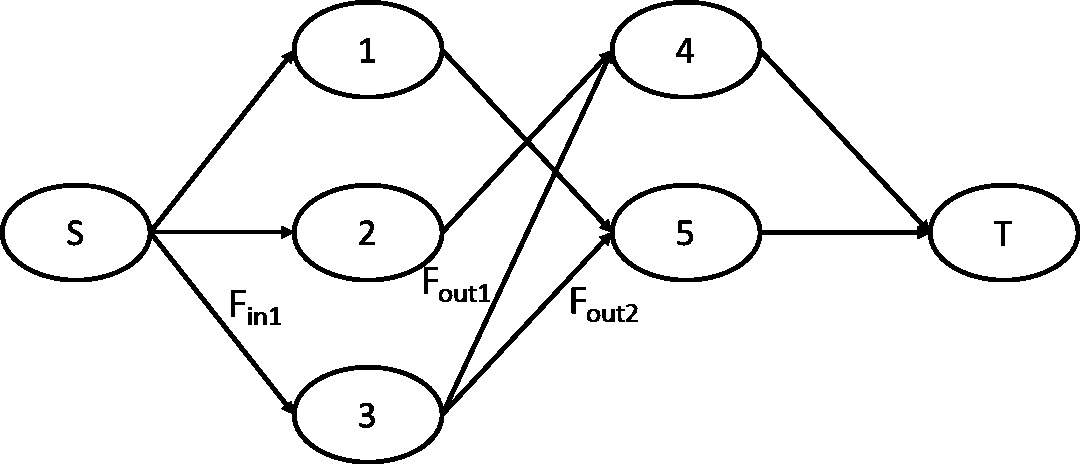
Two terms relating to the network are defined below, namely $F_{in}(n)$ ’s and $F_{out}(n)$ ’s of a node n in a flow network. The paper mentions them frequently.

Definition 1. ( $F_{in}(n)$ ’s and $F_{out}(n)$ ’s of a node n in a flow network): For a given node $n$ , the flows in its in-edges are called $F_{in}(n)$ ’s, and the flows in its out-edges are called $F_{out}(n)$ ’s.

For example in Fig. 1, the flow in edge S-3 is the only $F_{in}$ of node 3, and the flows in edges 3–4 and 3–5 are two $F_{out}$ ’s of node 3.

For a given flow network, there are three properties described below.

The flow in an edge must be equal to or smaller than the capacity.

For a given intermediate node $n$ , the summation of values of all $F_{in}(n)$ ’s must equal the summation of all $F_{out}(n)$ ’s. For example, in node 3 of Fig. 1, $F_{in1}=F_{out1}+F_{out2}$ .

The summation of values of all $F_{out}(S)$ ’s of node $S$ must equal the summation of all $F_{in}(T)$ ’s of node $T$ .

3.2 Lattice of frequent itemsets

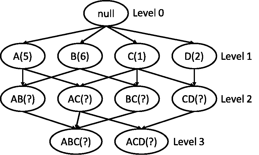
In a lattice of frequent itemsets, only the itemsets with their frequencies equal to or larger than the given minimum support threshold are kept. A special value null is put at the only node at level 0, and there is a directed edge between the null node and each node with a frequent itemset containing only one item at level 1. The content of a node at each level contains a frequent itemset with their item number the same as the level number, and the itemsets are arranged according to the alphabetical order. There is a directed edge between two nodes at neighboring levels, if one itemset can fully contain the other. Figure 2 shows an example of a lattice. For example, there is a directed edge between $A$ and AB because AB can fully contain $A$ , and they are at two neighboring levels. The numbers beside the itemsets denote their supports, and the question symbols represent the supports are unknown.

A term relating to the lattice is defined below, namely relating itemsets of an itemset in a lattice, which will be mentioned again in other sections.

Definition 2. (Relating itemsets of an itemset in a lattice): Relating itemsets of an itemset are the itemsets that there is a directed edge connecting to the itemset.

For example in Fig. 2, the relating itemsets of AB are $A$ and $B$ since there are directed edges between AB and each of $A$ and $B$ .

3.3 Simple flow network of frequent itemsets

A simple flow network is transformed from a lattice of frequent itemsets, with the content and the order of each level fully corresponding to those in the lattice, and two nodes $S$ and $T$ added to the network. The node null in the lattice is not put to the network. Figure 3 shows an example of the network, which is transformed from Fig. 2. Note that, since structure and content of the simple network fully correspond to the lattice; hence, relating itemsets of an itemset in the network are same with the itemset in the lattice. About other details of the simple network, they are described in following paragraphs.

Figure 3.

A simple flow network of frequent itemsets.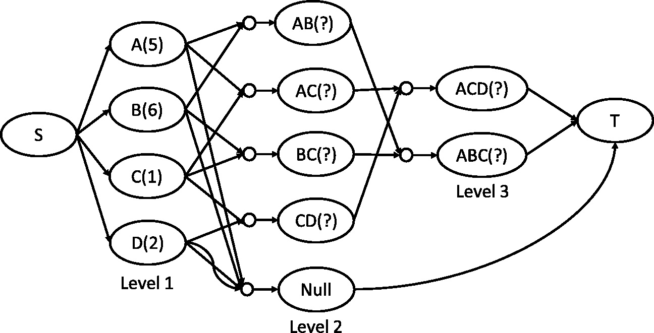

The paragraph describes the edges relating to the two special nodes ( $S$ and $T$ ). The node $S$ links to each itemset at level 1, and the capacity of each edge is the support of the 1-itemset indicated by the edge. Each itemset at the last level links to node $T$ with an edge of infinite capacity. For example in Fig. 2, the capacity of the edge $S-A$ is 5 since the support of the itemset $A$ is also 5. Capacities of the other edges starting from the node $S$ can be derived in the same way. Besides, the capacities of both the two edges ACD-T and ABC-T are infinite.

In the simple network, except the two special nodes ( $S$ and $T$ ), there is another kind of special node, namely collecting node. The node is defined below, and it is mentioned frequently in other sections.

Definition 3. (Except $S, T$ and all itemsets at level 1, collecting node of each itemset and the edges relating to the node): Except all itemsets at level 1 and the two special nodes ( $S$ and $T$ ), left side of each itemset is putted into a collecting node. For two neighboring levels, each itemset at left level of the two levels links to collecting nodes of the itemsets at the right level with edges of infinity capacity, if the itemset can be fully contained by the itemsets. Note that the collecting nodes are represented as small circles.

For example in Fig. 3, $C$ at level 1 links to the collecting nodes of AC, BC and CD at level 2, since these itemsets can fully contain $C$ . Except $S$ , $T$ and the itemsets at the last level of a simple flow network, the out-degree of each itemset at a same level is requested to keep consistent. Here, the consistence means they have the same out-degrees. For example in Fig. 3, the nodes at level 1 have different out-degrees, if the edges relating to the node of Null at level 2 are deleted. The out-degrees are ( $A$ , 2), ( $B$ , 2), ( $C$ , 3) and ( $D$ , 1), respectively, where the first elements of the pairs are the itemsets at level 1, and the second elements are the out-degrees of the itemsets. When the edges linked to the node of Null are added to Fig. 3, the out-degrees of the itemsets at level 1 all are same, namely the out-degrees at level 1 keep consistent. How to keep consistent for the out-degrees of the itemsets at a same level is described below.

For a level in the simple network, a special node Null is added to the next (right) level of the level, and each itemset at the left level links to the node with $N$ additional edges of infinite capacity, to keep consistency of the out-degrees at the left level. The value of $N$ is calculated with the following method. Given an itemset at the left level, let deg represent the out-degree of the itemset and max_deg represent the maximum out-degree of the left level. The itemset needs additional (max_deg –deg) edges to keep consistency of the out-degrees. Note that, the Null must link to $T$ with infinite capacity.

For example at level 1 of Fig. 3, the max_deg of the level is 3 if we ignore the edges linking to the node Null at level 2, and the itemset that has the out-degree is $C$ . In order to keep same out-degree for each itemset at the level, the itemset $D$ must link to the node Null with 2 additional edges. The edge number 2 is derived because the max_deg is 3 and its out-degree (deg) is 1. The similar concept can be applied to the itemsets $A$ and $B$ .

3.4 Complex flow network of frequent itemsets

The complex network is extension of the simple network. Two additional factors are added to the complex network, namely interval and correcting edge pair, and they are described in Definitions 4 and 5, separately. Figure 4 shows an example of the complex network. Note that, the two factors are represented by dotted lines.

Definition 4. (Intervals at a level of the complex network): An order number is attached to an itemset at a level. From the upmost node to bottommost node, the itemsets are numbered $1,2,3,\ldots,n$ , separately, where $n$ is the number of the itemsets at that level. An interval contains a set of itemsets that their order numbers are continuous (the difference of the order numbers of any two near itemsets in the interval is 1). Note that, an interval can be represented by the two border itemsets in the interval.

For example in Fig. 4, level 2 contains two intervals, namely [AB, AC] and [BC, CD]. The number of AB is 1, of AC is 2, and the difference of the numbers of the two near itemsets is 1. Situation of [BC, CD] is similar to [AB, AC].

Definition 5. (The correcting edge pairs in the complex network): For each collecting node, an edge pair is added to the node. One of the two edges is from $S$ to the node, and another one is from the node to $T$ . Except the level 1, the itemsets at the other levels are partitioned into intervals. The capacities of the correcting edge pairs have the same value pair if the pairs are in the same interval. Note that, the Null nodes are not contained by any interval.

Figure 4 shows an example of a complex flow network. Note that, the correcting edge pairs at level 3 are not shown for simplicity. The itemsets AB and AC at level 2 of the figure are at same interval; hence, correcting edge pairs of the two itemsets have same value pair, namely ( $C_{1},C_{2}$ ). Situation of the two itemsets BC and CD is similar to AB and AC.

Figure 4.

A complex flow network of frequent itemsets.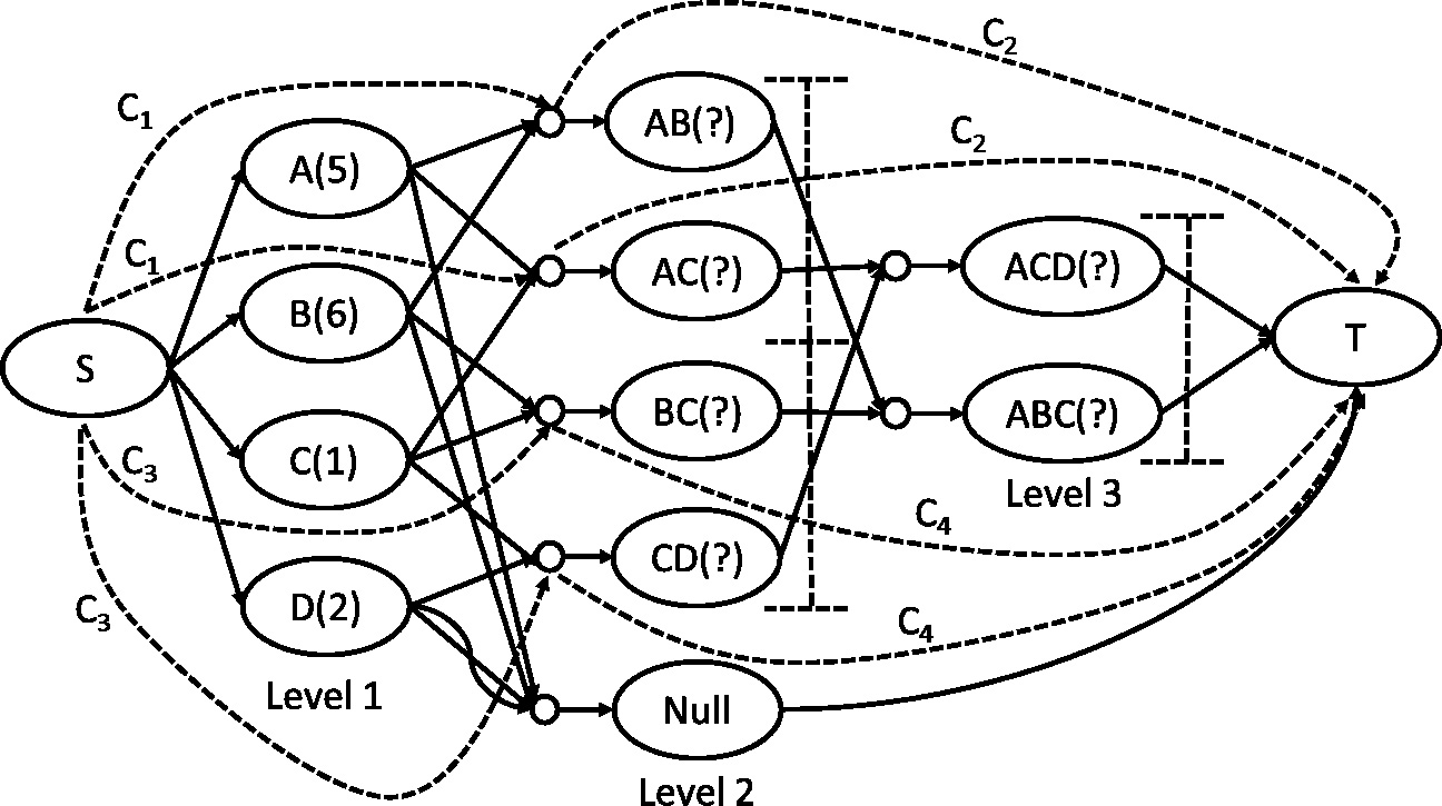

4. Preliminary observations and problem statement

For a given lattice of frequent itemsets, assume supports of the itemsets at level 1 are known and supports of the itemsets at the other levels are unknown. A simple heuristic can be applied to predict the unknown supports from the known supports. The heuristic is based on the observation among the itemsets at any two near levels of the lattice, which is described in Observation 1. In the paper, this concept is implemented through a flow network.

Observation 1. (For the itemsets at any two near level of the lattice, except level 0 and level 1, supports of the itemsets at bottom level of the two levels can be distinguished by their relating itemsets at the top level): For the itemsets at the bottom level, an itemset may be larger than that of another itemset at same level with a high probability, if supports of the relating itemsets (described in first paragraph of Section 3.3) of the itemset mostly are larger than those of the latter.

For example in Fig. 2, the relating itemsets of AB are $A$ and $B$ , and those of CD are $C$ and $D$ . Support of AB may be larger than CD, since supports of $A$ and $B$ are also larger than supports of $C$ and $D$ .

Observation 1 has shown the phenomenon, and it is also known that the content and structure of the simple network fully correspond to the lattice. At any two near levels of the simple network, except the levels between $S$ and level 1 and last level and $T$ , can the supports of the itemsets at the right level of the two levels be distinguished by the supports at the left level? It is described in Observation 2. In order to let the simple network can reach the request, the values of all F ${}_{out}(I)$ ’s of each itemset $I$ (except $S$ , $T$ and the itemsets at the last level) in the simple network must be defined. It is described in Definition 6.

Definition 6. (Except $S, T$ and the itemsets at the last level, the values of all $F_{out}(I)$ ’s of each itemset $I$ in the simple network): Let $F_{in\_total}$ be the summation of values of all $F_{in}(I)$ ’s of an itemset $I$ , and out_degree represent out-degree of $I$ . The value of each $F_{out}(I)$ of $I$ is defined as $F_{in\_total}$ /out_degree. Note that, if the values of $F_{out}(I)$ ’s are not integers, rounding is applied.

For example, in Fig. 3, the $F_{in\_total}$ value of the itemset $B$ is 6, and its out-degree is 3. The value of each $F_{out}$ of the itemset is 6/3, which is 2.

Observation 2. (For the itemsets at any two near levels of the simple network, except S and level 1, and last level and T, the supports of the itemsets at the right level of the two levels can be distinguished by their relating itemsets at the left level): According to the description of Definitions 6 and last two paragraphs in Section 3.3, the out-degrees of the itemsets at the left level are the same, and all the values of their $F_{out}$ ’s are defined as $F_{in\_total}$ /out_degree. Hence, for the itemsets at the left level, if the support of an itemset is larger than those of other the itemsets, then its each $F_{out}$ is also larger than those of other the itemsets. Based on the reason above, if supports of the relating itemsets of an itemset at the right level are large, then the only $F_{out}$ of the correcting node of the itemset is also large, since the only $F_{out}$ is the summation of all the $F_{out}$ ’s (on the edges linking to the correcting node) of the relating itemsets. It is consistent with Observation 1.

Take level 1 and level 2 in Fig. 3 as an example. The relating itemsets of the itemset AB are $A$ and $B$ , those of CD are $C$ and $D$ , and the supports of $A$ and $B$ are larger than those of $C$ and $D$ . According to the description of Observation 2, the value of the only $F_{out}$ of the correcting node of AB must be larger than that of the only $F_{out}$ of CD.

A simple flow network can only distinguish the frequent itemsets, but it does not exactly predict the support of each itemset. In order to reach the purpose, we expand the simple flow network to the complex flow network. Before discussing why the complex network can closely predict supports of the itemsets in detail, some terms must be defined.

Definition 7. (Distinguishing flow $F_{dist}$ of each correcting node in the complex network): Eliminating the effect by all flows in the correcting edge pairs, the only $F_{out}$ value of a correcting node is called as distinguishing flow $F_{dist}$ . Note that, the property of the $F_{dist}$ corresponds to the only $F_{out}$ of correcting node of the itemset in the simple network. It is described in Observation 2.

Definition 8. (Correcting flows $F_{corr}(n)$ ’s of each correcting node $n$ in the complex network): The flows in correcting edge pair of the correcting node $n$ are called as correcting flows $F_{corr}(n)$ ’s.

Definition 9. (Except the itemsets at level 1 of the complex network, predicted support (flow) of each itemset): The predicted flow of an itemset is the only $F_{out}$ (enter to the itemset) value of correcting node of the itemset. According to the property of the network (described in Section 3.1), if the capacity of the correcting edge starting from $S$ is increased, then the flow is increased as well; if the capacity of the correcting edge ending at $T$ is increased, then the flow is decreased. Let $F_{corr\_s}$ represents the correcting flow starting from $S$ , and $F_{corr\_t}$ represents the correcting flow ending in $T$ , the predicted support can then be defined as $F_{dist}+F_{corr\_s}-F_{corr\_t}$ .

Definition 9 discusses the predicted flows of the itemsets in a complex network, and the method which adjusts the predicted flow of each itemset in the network is also discussed. A question is, whether a complex flow network can be used to get close predicted flow of each itemset? The answer is sure if the intervals in a complex network are put to suitable locations, and the details are shown in Observation 3. How to set the capacities of the edge pairs and to find the best intervals are described in Sections 5.1 and 5.2, respectively.

Observation 3. (The complex flow network can be used to get close predicted flows of the itemsets): Fig. 5 shows an example to explain the phenomenon. In the example, all the itemsets at level 2 of Fig. 4 are partitioned into two intervals, namely [AB, AC] and [BC, CD]. The left interval of Fig. 5 represents [AB, AC], and the right interval represents [BC, CD]. $F_{real}$ (AB) and $F_{real}$ (AC) represent real supports of AB and AC, separately; $F_{dist}$ (AB) and $F_{dist}$ (AC) represent the distinguishing flows of correcting nodes of AB and AC in Fig. 4, separately. $F_{dist}$ (AB) is larger than $F_{dist}$ (AC), since supports of the relating itemsets of AB are larger or equal than those of AC. Situation of the right interval is similar to the left interval. According to the description of Definition 7 and Observation 2, the $F_{dist}$ ’s in Fig. 5 should be consistent with the corresponding $F_{real}$ ’s. For example, left interval of Fig. 5, $F_{rea1}$ (AB) is larger than $F_{real}$ (AC), since $F_{dist}$ (AB) is larger than $F_{dist}$ (AC). For the left interval, $F_{dist}$ (AB) and $F_{dist}$ (AC) are assumed much higher than $F_{real}$ (AB) and $F_{real}$ (AC), separately. According to description of Definition 9 (Predicted support of an itemset $I$ can be represented as $F_{dist}(I)+F_{corr\_s}(I)-F_{corr\_t}(I)$ ), and Definition 5 (the $F_{corr\_s}$ ’s and $F_{corr\_t}$ ’s in same interval have same value pair, and they are represented as $F_{corr\_s}$ and $F_{corr\_t}$ , separately), $F_{dist}$ (AB) and $F_{dist}$ (AC) can be close to $F_{real}$ (AB) and $F_{real}$ (AC), separately, if the $F_{corr\_t}$ of AB and AC is increased. Similar derivation is applied to the right interval, in which the $F_{corr\_s}$ of BC and CD must be increased.

Figure 5.

Adjusting capacities on the collecting edge pairs to make 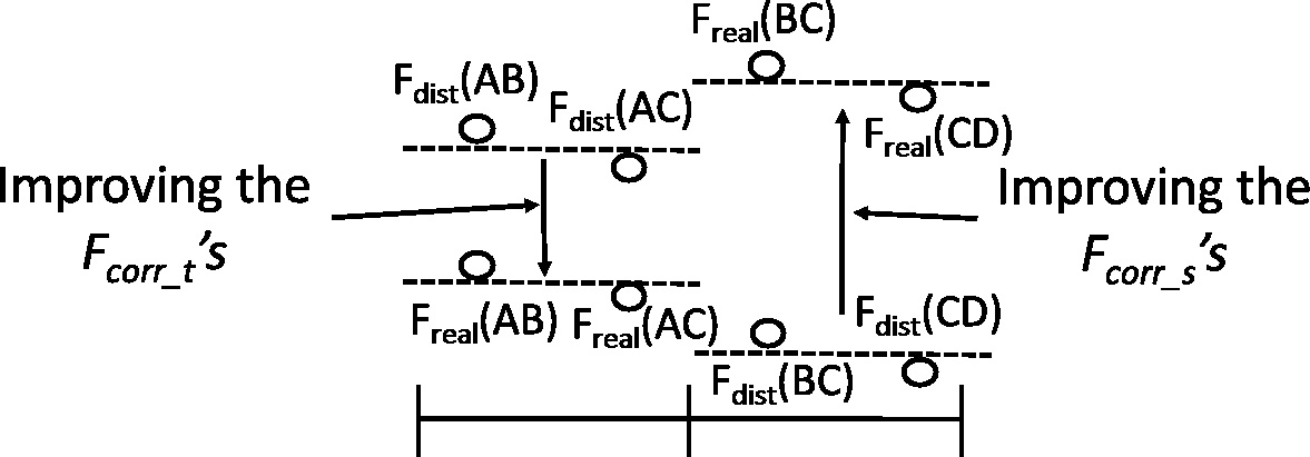$F_{dist}$ ’s close to their $F_{real}$ ’s.

In summary, the purpose of the paper is to reduce the information for storing frequent itemsets and their frequencies. For a set of given frequent itemsets, only the maximal itemsets, all frequent 1-itemsets and the intervals, are saved, instead of all the frequent itemsets. The itemsets and their approximate supports can be recovered through the following steps: 1. recovering the lattice of frequent itemsets using the maximal itemsets, 2. rebuilding the complex flow network using the 1-itemsets and intervals, and 3. obtaining the close support of each itemset according to the properties of the complex network. Note that the maximal itemsets know their real supports; hence, they are not put into the complex network.

5. Proposed concepts and methods

In the section, we describe our methods in details. Section 5.1 describes how to set capacities of the correcting edge pairs in the complex network, and Section 5.2 describes how to identify the best intervals at a level of the complex network.

5.1 Setting capacities of correcting edge pairs

According to the description of Observation 3, the predicted support of the itemsets in an interval can be close to their real supports, if the values of the $F_{corr\_s}$ ’s and $F_{corr\_t}$ ’s are set correctly $.$ In the section, we describe how to set the capacities of the correcting edge pairs to make the predicted support of each itemset close to its real support. The measure for the predicted flow of an itemset close to its real support can be calculated by Eq. 1. Note that, the values of $F_{corr\_s}$ ’s and $F_{corr\_t}$ ’s in an interval have same value pair of capacities; hence, the $F_{corr\_s}$ ’s and $F_{corr\_t}$ ’s are represented as $F_{corr\_s}$ and $F_{corr\_t}$ , separately.

$\textit{Error}=\sum\limits_{i=1}^{n}\left(F_{dist}(i)+F_{corr\_s}(i)-F_{corr\_% t}(i)-\textit{Real\_Support}(i)\right)^{2}$ (1)

where $n$ represents the number of the itemsets in an interval. If the predicted flows are close to their corresponding real supports, then the error is small; on the contrary, the error is large.

Before discussing how to assign the capacities in details, Eq. 2 and some theorems relating to the formula are introduced, which is useful to understand the problem.

$\textit{Condition}=\sum\limits_{i=1}^{n}\left(F_{dist}(i)-\textit{Real\_% Support}(i)\right)$ (2)

where $n$ represents the number of the itemsets in an interval. The condition in Eq. 2 is related to setting $F_{corr\_s}$ and $F_{corr\_t}$ in an interval. The reason is described in Theorem 1.

Theorem 1. When the condition is a positive number, value of $F_{corr\_s}$ of all the itemsets in an interval must be 0, and value of $F_{corr\_t}$ of all the itemsets must be positive numbers; when the condition is a negative number, the $F_{corr\_s}$ must be positive numbers, and the $F_{corr\_t}$ must be 0; when the condition is 0, then the $F_{corr\_s}$ and $F_{corr\_t}$ must be 0.

In Theorem 1, when the condition is a positive number, most values of the $F_{dist}$ ’s in an interval are larger than their corresponding real supports. Hence, value of the $F_{corr\_t}$ must be increased to reduce the predicted flows (according to description of Definition 9). Similar concept is applied to the opposite situation. If the condition is 0, then the $F_{dist}$ ’s reach a balance point, and increasing or decreasing the $F_{corr\_s}$ and $F_{corr\_t}$ is not useful for getting better predicted flows. Theorem 2 describes how to set in Eq. 2 the two values, $F_{corr\_s}$ and $F_{corr\_t}$ , in an interval.

Theorem 2. When the condition value is a non-zero number, values of the optimizing 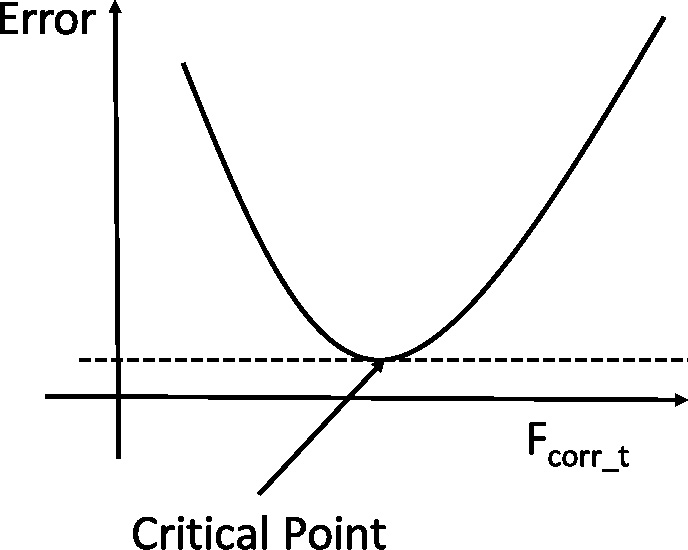$F_{corr\_s}$ and $F_{corr\_t}$ are at the critical point of Eq. 1.

In Theorem 2, when the condition value is a positive number, most values of $F_{dist}$ ’s are larger than their corresponding real supports. Hence, values of the $F_{corr\_t}$ must be increased to make the prediction flows close to the real supports. When the $F_{corr\_t}$ increases continuously, value of the Error decreases at the beginning and then turns to increasing when the $F_{corr\_t}$ overly increases. Figure 6 shows the concept. Similar concept can be applied to the opposite situation.

Figure 6.

The optimizing $F_{corr\_t}$ is at the critical point.

Based on the above discussions, if the condition is a positive number, optimizing value of the $F_{corr\_t}$ can be calculated by Eq. 3:

$F_{corr\_t}=\sum\limits_{i=1}^{n}\left(F_{dist}(i)-\textit{Real\_Support}(i)% \right)/n$ (3)

The opposite situation can be calculated with Eq. 4:

$F_{corr\_s}=\sum\limits_{i=1}^{n}\left(\textit{Real\_Support}(i)-F_{dist}(i)% \right)/n$ (4)

where $n$ represents the number of the itemsets in an interval. The following theorems can thus be derived.

Theorem 3. When the condition value is a positive number, the optimizing $F_{corr\_t}$ can be calculated by Eq. 3.

Proof

$\displaystyle\frac{d\textit{Error}}{dF_{corr\_t}}=0$ $\displaystyle=>\left(\sum\limits_{i=1}^{n}\left(F_{dist}(i)+0-F_{corr\_t}-% \textit{Real\_Support}(i)\right)^{2}\right)^{\prime}=0$ $\displaystyle=>\sum\limits_{i=1}^{n}{2\left(F_{dist}(i)-F_{corr\_t}-\textit{% Real\_Support}(i)\right)\left(-1\right)}=0$ $\displaystyle=>\sum\limits_{i=1}^{n}{2\left(\textit{Real\_Support}(i)+F_{corr% \_t}-F_{dist}(i)\right)}=0$ $\displaystyle=>2nF_{corr\_t}+2\sum\limits_{i=1}^{n}{\left(\textit{Real\_% Support}(i)-F_{dist}(i)\right)=0}$ $\displaystyle=>F_{corr\_t}=\sum\limits_{i=1}^{n}\left(F_{dist}(i)-\textit{Real% \_Support}(i)\right)/n$

Theorem 4. When the condition is a negative number, the optimizing $F_{corr\_s}$ can be calculated with Eq. 4

Proof

$\displaystyle\frac{\textit{Error}}{dF_{corr\_s}}=0$ $\displaystyle=>\left(\sum\limits_{i=1}^{n}\left(F_{dist}(i)+F_{corr\_s}-0-% \textit{Real\_Support}(i)\right)^{2}\right)^{\prime}=0$ $\displaystyle=>\sum\limits_{i=1}^{n}{2\left(F_{dist(i)}+F_{corr\_s}-\textit{% Real\_Support}(i)\right)}=0$ $\displaystyle=>\sum\limits_{i=1}^{n}{-2\left(\textit{Real\_Support}(i)-F_{corr% \_s}-F_{dist}(i)\right)}=0$ $\displaystyle=>2nF_{corr\_s}-2\sum\limits_{i=1}^{n}{\left(\textit{Real\_% Support}(i)-F_{dist}(i)\right)=0}$ $\displaystyle=>F_{corr\_s}=\sum\limits_{i=1}^{n}\left(\textit{Real\_Support}(i% )-F_{dist}(i)\right)/n$

5.2 Dividing the itemsets at a level as intervals

For a level of the complex network, Section 5.1 has shown how to set capacities of the correcting pairs to make the predicted flows close to their real supports. The section then introduces how to efficiently put the intervals to suitable locations. Before introducing how to find the best intervals, some definitions about the representation of an interval are first given below.

Definition 10. (Default cuttings of a level in the complex network): Each level in the complex network contains two default cuttings, which are put into top of the topmost itemset and bottom of the bottommost itemset, and the two default cutting can be represented as the two itemsets, separately. Note that, the Null node is excluded from the bottommost itemset, and each level can be represented with the default cuttings

For example in Fig. 4, the default cuttings of level 2 are put into top of [AB] and bottom of [CD], respectively, and the two cutting are represented as [AB] and [AC], separately. The level 2 can be represented as [AB, CD].

Definition 11. (Cutting of a level in the complex network): Cutting is put in middle of two neighboring itemsets at a level, and the cutting can be represented with the two itemsets. For example in Fig. 4, level 2 contains a cutting [AC, BC].

Definition 12. (Number of cutting and default cuttings in the complex network): According to description of Definitions 10 and 11, the cuttings can be put the locations at a level of the complex network, namely top of the top itemset, bottom of the bottom and the middle between any two neighboring itemsets. Each of the locations is given a number. The topmost location is given 0, the middle between the first (topmost) and the second itemsets is given 1, and so on. The bottommost location is given $N$ , where $N$ is the number of the itemsets at the level. Since the cuttings are also put in the locations, numbers of the cuttings are also numbers of the locations. For example in Fig. 4, the number of the cutting [AB] is 0, of [AC, BC] is 2, and of [CD] is 4.

Definition 4 shows the definition of the interval. It is clear that an interval can be represented by a pair of the itemsets, which consists of top-boundary-cutting and bottom-boundary-cutting of it. Definition 12 shows that the cuttings can be represented as the numbers. Based on the two reasons, an interval can thus be represented as a pair of the numbers of the top-boundary-cutting and bottom-boundary-cutting. Note that, the number of the itemsets contained in an interval or at a level can be calculated by the difference of the numbers of the two cuttings, namely Number(bottom-boundary-cutting) $-$ Number(top-boundary-cutting). For example in Fig. 4, the two intervals at level 2 can be represented as [0, 2] and [2, 4]. Similar to an interval, a level can be represented as a pair of the numbers of the two default cuttings. For example in Fig. 4, level 2 can be represented as [0, 4].

Our methods relate to the Eqs 5–10, which are described below in detail. The number of the cuttings at a level can be specified by Eq. 5 as follows:

$\textit{Cuttings}=\left\lfloor C\times\textit{Intermediate\_Nodes}\right% \rfloor+1$ (5)

where $C$ is a given real number in the interval of 0 to 1, and Intermediate_Nodes represents the number of the itemsets at the level. Small $C$ values represent fewer intervals than large $C$ values, which also means less information is used to store the supports of the itemsets and the predicted flows are far from the real supports. Contrary to small $C$ values, large $C$ values bring accurate predicted flows, but much information is needed.

Given the number of the cuttings, it is important to put the cuttings to correct the locations (described in Definition 11) to make the predicted flows as close to the corresponding real supports as possible. The problem can be viewed as a series of decision of optimization-binary-division. First, a cutting is put to a location of a level to allow the itemsets divided into two disjoint parts. The cutting is expected as an optimization partition, which means it can make the summation of the minimum errors of the top part and the bottom part of the cutting minimum. How to calculate the minimum errors of the two parts, which can apply similar operation to the two parts, separately. The concept above can be summarized as shown in Eq. 6:

$\textit{Error}\left(0,N,K\right)={\min}_{{\begin{subarray}{l}0\leqslant i<N\\ 0\leqslant j<K\\ \end{subarray}}}\left\{\textit{Error}\left(0,i,j\right)+\textit{Error}(i,N,% \left(K-1\right)-j)\right\}$ (6)

where the term Error $(0,N,K)$ represents the minimum error of a level. $N$ represents the number (described in Definition 12) of the bottom-boundary-cutting of the level. $K$ represents maximum number of the cuttings assigned to the level, and it can be calculated by Eq. 5. The first value of the triple represents the number of the top-boundary-cutting. Error $(0,i,j)$ represents the top part of the binary-division, $i$ represents the number of the top-boundary-cutting, and $j$ represents the number of the cuttings assigned to the part. Error $(i,N,(K-1)-j)$ is similar to Error $(0,i,j)$ , except different parameter values. Note that, the two triples Error $(i,N,(K-1)-j)$ and Error $(0,i,j)$ can be viewed as sub-problems of the triple Error $(0,N,K)$ .Equations 7–10 shows initial conditions of the recursive execution in Eq. 6.

$\displaystyle\textit{Error}\left(i,j,K\right)=\textit{impossible},j-i\leqslant 0$ (7) $\displaystyle\textit{Error}\left(i,j,0\right)=\textit{formula}\_1$ (8) $\displaystyle\textit{Error}\left(i,j,K\right)=0,j-i=1$ (9) $\displaystyle\textit{Error}\left(i,j,K\right)=0,j-i-1\leqslant K$ (10)

Equation 7 represents the top boundary must be above the bottom boundary, and the number of the itemsets contained by an interval must be more than or equal to 1; otherwise, the interval is illegal.Equation 8 represents the error of the interval can be calculated if the number of the cuttings assigned to the interval is 0, and it is related to Section 5.1.Equation 9 represents the error must be 0 if the number of the itemsets contained in the interval is 1. The reason is shown in Theorem 3 below.Equation 10 represents that the error must be 0 if the number of the cutting assigned to the interval is enough to let each sub-interval only contain an itemset. The reason is shown in Theorem 4 below.

Theorem 3. When the number of the itemsets at an interval is 1, the minimum error of the interval must be 0.

According to Eq. 1, the error of the interval can be written as $F_{dist}+F_{corr\_s}-F_{corr\_t}$ $-$ Real_Support. In the theorem, since the error is considered as 0, the formula can thus be written as Real_Support $=$ $F_{dist}+F_{corr\_s}-F_{corr\_t}$ . According to the principle of setting $F_{corr\_s}$ and $F_{corr\_t}$ (Theorem 1), the error can be re-written as Real_Support $=$ $F_{dist}+F_{corr\_s}$ or Real_Support $=$ $F_{dist}+F_{corr\_t}$ , where, both $F_{dist}$ and Real_Support are known constant and both $F_{corr\_s}$ and $F_{corr\_t}$ are unknown. It is clear that both the two formulas are first-degree polynomials with one variable; hence, the solution of the two unknown variables $F_{corr\_s}$ and $F_{corr\_t}$ must exist. It also means the theorem is valid.

Theorem 4. When the number of the cuttings assigned to an interval is enough to make each sub-interval only contain an itemset, the error of the interval must be 0. Note that, if the number of the itemsets in the interval is $N$ , then the interval only needs $N-1$ cutting to generate the sub-intervals.

In the situation of Theorem 4, an interval at a level can be divided into a set of the sub-intervals that only contain an itemset. According to Theorem 3, the errors of all the sub-intervals are 0, and the error of the interval is the summation of the errors of the sub-intervals; hence, the theorem is valid.

In the paper, the concept of dynamic programming is applied to solve the problem. A 3-dimensional array is used to save results of the sub-problems, and each element of the array represents result of a triple Error $(i,j,k)$ . The $x$ -index of the array represents the $i$ value (the number of the top boundary of an interval), the $y$ -index represents the $j$ value (the number of the bottom boundary of an interval), and the $z$ -index represents the $k$ value (the number of the cuttings assigned to the interval). Before discussing how to identify the best intervals, a term and a theorem relating to the array will be described in details below.

Definition 13. (K-slice of the 3-dimensional array): The $K$ -slice of the 3-dimensional array represents a set of elements in which all the z-index values are $K$ , namely the elements ( $i, j, K$ ) in the array, where, 0 $\leqq i<$ height of the array, 0 $\leqq j<$ width of the array. Note that, the height is the maximum value of the $x$ -index, and the width is the maximum value of the $y$ -index.

Theorem 5. Before calculating a triple Error $(i,j,k)$ , the results of elements in the K-slices $(K<k)$ must be known.

Observing the top part (Error $(0,i,j)$ ) and the bottom part (Error $(i,N,(K-1)-j)$ ) in Eq. 6, and the range of variable $j$ ( $0\leqq j<K$ ), It is clear that the theorem is valid.

Figure 7 shows the details of the algorithm. It numerates the $K$ -slices from small $K$ values to large $K$ values, based on Theorem 5. The output of the algorithm is in the element ( $0,N,K$ ) of the array since the element represents Error( $0,N,K$ ). That is, the minimum error of a level on the condition that the number of the permitted cuttings is $K$ .

Figure 7.

The algorithm for mining best intervals at a level of the complex network.

6. Experiments

The section contains the two sub-sections, namely Experimental Datasets and Criteria (Section 6.1) and, Experimental Results (Section 6.2). Section 6.1 explains the sources and generation of datasets used in the paper and uses three criteria of performance. Section 6.2 demonstrates the performance of our method on different datasets and parameter values. Besides, the performance of the approaches of closed and maximal itemsets is also included to make a comparison with the proposed method.

6.1 Experimental datasets and criteria

Three criteria are used to evaluate approximate representation of frequent itemsets. They are representation rate (Eq. 11), error (Eq. 12), and running time.

The representation rate is defined as follows:

$\textit{representation\_rate}=\left(\textit{Intervals}+\textit{Items}+\textit{% MIs}\right)/{N\times 100\%}$ (11)

where Intervals represents the number of all intervals in the complex network, Items represents the number of all frequent 1-itemsets, MIs represent maximal itemsets and $N$ represents the number of all frequent itemsets.

The error is defined as follows:

$\textit{error}=\frac{\sum\nolimits_{i\in\textit{CIs}}\left(\left|p_{i}-a_{i}% \right|/{a_{i}\times 100\%}\right)}{N}$ (12)

where CIs represents the itemsets in any interval, $p_{i}$ and $a_{i}$ represent the predicted support and the real support of the $i$ -th itemset in CIs, and $N$ is the number of all frequent itemsets.

Representation rate shows how much data is needed for representing the list of given frequent itemsets and their approximate supports. A smaller representation rate represents the information which needs to be stored is less than a larger one. Error represents the summation of distances among real supports and predicted supports of given frequent itemsets. A smaller error is more desired than a larger one. Let $G$ represent a set of given frequent itemsets. According to the description in Section 4, the proposed method represents $G$ with three kinds of stored factors, namely 1-itemsets of $G$ , maximal itemsets of $G$ and several pairs of intervals in a complex flow network corresponding to $G$ . The number of the 1-itemsets and the maximal itemsets is constant when a dataset and a minimum support are specified. Since the $C$ value in Eq. 5 is used to directly reflect representation rate, therefore, the following experiments do not show representation rates for the different factors. Only the results relating to error and running time are shown.

Table 1

The ratios of maximal itemsets and closed itemsets in the six datasets

Datasets	Minimum	Frequent	Maximal	Closed
	supports	itemsets	itemsets	itemsets
Accidents	1950	1385	3.177%	49.675%
Accidents	1750	3025	3.008%	49.455%
Accidents	1600	5487	2.479%	48.916%
Pumsb	2650	1342	6.483%	42.176%
Pumsb	2580	3207	4.365%	33.801%
Pumsb	2540	5026	3.144%	29.686%
Pumsb_star	1300	1626	2.399%	28.598%
Pumsb_star	1260	3488	1.147%	17.747%
Pumsb_star	1230	5786	0.847%	12.876%
Chess	2650	1758	3.527%	65.131%
Chess	2570	3495	3.405%	60.315%
Chess	2500	5682	2.499%	56.441%
Mushroom	1800	1199	1.001%	3.003%
Mushroom	1400	3471	0.576%	2.218%
Mushroom	1200	5407	0.721%	2.423%
Connect	2999	1279	0.313%	0.391%
Connect	2998	3071	0.228%	0.391%
Connect	2997	5119	0.156%	0.391%

Table 2

The multipliers of error and running time in the six datasets

Datasets	Minimum	Multiplier	Multiplier
	supports	(error)	(running time)
Accidents	1950	4.48	2580
Accidents	1750	4.985	67847
Accidents	1600	5.547	783669
Pumsb	2650	1.197	2641
Pumsb	2580	1.187	89130
Pumsb	2540	1.204	669604
Pumsb_star	1300	6.676	4235
Pumsb_star	1260	4.739	85177
Pumsb_star	1230	3.436	706315
Chess	2650	1.174	6454
Chess	2570	1.226	91866
Chess	2500	1.247	893079
Mushroom	1800	4.878	1109
Mushroom	1400	6.924	70816
Mushroom	1200	9.425	582250
Connect	2999	0.00552	1047
Connect	2998	0.00757	34660
Connect	2997	0.00802	336713

Subsets of the six datasets were involved in the experiments, namely Accidents, Pumsb, Pumsb Star, Chess, Mushroom and Connect. The six datasets could be found in the website http://fimi.ua.ac.be/data/. The subsets were formed from the first 3000 records in the original datasets with the first 50 items that appeared in the datasets. If a record did not contain any of the items, then the record was not included within the original 3000 records; hence, additional records were selected until the number of the records arrived at 3000. Note that the original datasets do not contain any noise and missing values.

The testing program was written in Java. The environment for software development is as follows. The OS is Microsoft Windows 8.1 $\times$ 86_64, the version of Java Runtime Environment is 8.0 build 60 $\times$ 86_64, and the hardware is an Intel Core i5 2300 (CPU) with DDR3 1333 8 GB memory (4G $\times$ 2, Dual Channels).

Figure 8.

The errors for datasets accidents and pumsb.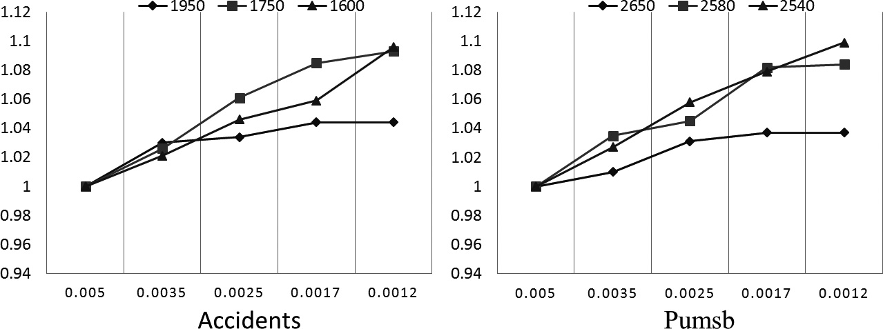

Figure 9.

The errors for datasets pumsb_star and chess.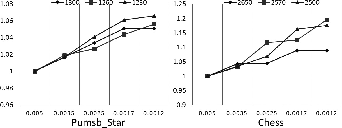

Figure 10.

The errors for datasets mushroom and connect.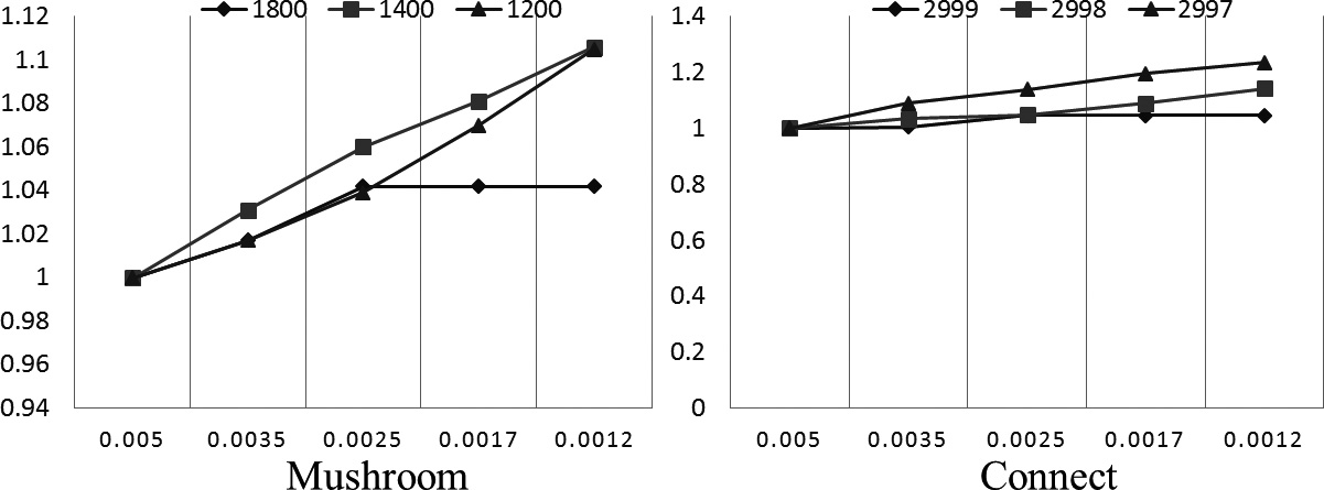

6.2 Experimental results

Table 1 shows numbers of frequent itemsets, and the ratios of closed itemsets and maximal itemsets in all frequent itemsets for different minimum support thresholds and datasets. It is notable that setting the minimum support values to the above values maintains consistency of numbers of the frequent itemsets.

Figure 11.

The running times for datasets accidents and pumsb.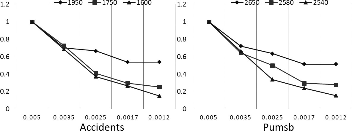

Figure 12.

The running times for datasets pumsb_star and chess.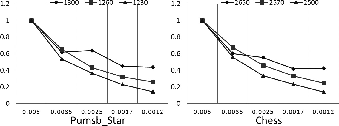

Figure 13.

The running times for datasets mushroom and connect.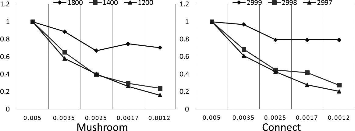

Figures 8–10 show the errors of the six datasets for the different factors, namely datasets, minimum supports and the $C$ values. The x-axles represent various $C$ values and the y-axles represent the errors. Note that, real value of the error for specified the factors equals to value of the y-axle multiply the multiplier of different datasets and minimum supports. The multipliers for the different datasets and minimum supports are showed in Table 2. For example, real value of the error for dataset is accidents, support is 1950 and $C$ is 0.0035 equals 1.03 $\times$ 4.48%, namely 4.614%. Note that, unit of the running times is micro second (ms).

Figures 11–13 then show the running times of proposed approach for the six datasets. The x-axles represent various $C$ and the y-axles represent the times. Similar to the above experiments, value of the real time for the different the factors equals to value of the y-axle multiply the multiplier. The multipliers are the same as those shown in Table 2.

According to the above results, a trend is clear, namely the running time decreases when the $C$ value decreases as well. It is because the $C$ value affects the number of the intervals, which then affects two of the five for-loops of the algorithm in Fig. 7. If the times that the for-loops repeat are many, then long running time is needed. Another trend is also interesting, namely the decreasing rate of the running time for a variety of $C$ values is larger than the increasing rate of the error. According to the above two trends, the proposed method is suitable when low representation rate (small $C$ value) is required.

7. Conclusion and future works

In this paper, we propose a new compact representation that lies between closed itemsets and maximal itemsets. It reserves all the frequent itemsets and identifies their approximate supports. A list of all frequent itemsets is first recovered through the maximal itemsets, and they are organized as the complex network. Next, the itemsets at each level of the network are partitioned into intervals except level 1. Through the information of the 1-itemsets and the intervals, the approximate supports of the itemsets in the intervals can be obtained. Experiments show the proposed method is suitable when low represent rate is requested. The proposed approach may be not efficient if we need very close approximate supports. It represents a trade-off between efficiency and accuracy. In the future, we will continue discovery on efficient division of a level to ensure the concept can fit in all kinds of situations. We will also make more experiments on more datasets and on other approaches such as non-derivable itemsets.

References

Agrawal

Imieliński

and Swami

, Mining association rules between sets of items in large databases, Proceedings of the ACM SIGMOD International Conference on Management of Data, (1993), 207–216.

Bayardo

R.J.

, Jr., Efficiently mining long patterns from databases, Proceedings of the ACM SIGMOD International Conference on Management of Data, (1998), 85–93.

Boulicaut

J.-F.

Bykowski

and Rigotti

, Free-sets: A condensed representation of boolean data for the approximation of frequency queries, International Journal of Data Mining and Knowledge Discovery 7(1) (2003), 5–22.

Calders

and Goethals

, Non-derivable itemset mining, International Journal of Data Mining and Knowledge Discovery 14(1) (2007), 171–206.

Chandola

and Kumar

, Summarization – compressing data into an informative representation, International Journal of Knowledge and Information Systems 12(3) (2007), 355–378.

Chiranjeevi

and Hari

, Modified GUIDE (LM) algorithm for mining maximal high utility patterns from data streams, International Journal of Computational Intelligence Systems 8(3) (2015), 517–529.

Gallo

De Bie

and Cristianini

, MINI: Mining informative non-redundant itemsets, Proceedings of the 11th Conference on Principles and Practice of Knowledge Discovery in Databases, (2007), 438–435.

Han

Pei

and Yin

, Mining frequent patterns without candidate generation, Proceedings of the ACM SIGMOD International Conference on Management of Data, (2000), 1–12.

Hipp

Güntzer

and Nakhaeizadeh

, Algorithms for association rule mining – a general survey and comparison, ACM SIGKDD Explorations Newsletter, (2000), 58–64.

10.

Huang

J.-N.

Hong

T.-P.

and Chiang

M.-C.

, Reference itemsets: Useful itemsets to approximate the representation of frequent itemsets, Soft Computing (2016), doi: 10.1007/s00500-016-2172-4.

11.

van Leeuwen

and Ukkonen

, Discovering skylines of subgroup sets, International Journal of Machine Learning and Knowledge Discovery in Databases 8190 (2013), 272–287.

12.

Lin

M.-Y.

T.-F.

and Hsueh

S.-C.

, High utility pattern mining using the maximal itemset property and lexicographic tree structures, Information Sciences 215 (2012), 1–14.

13.

Liu

Pan

Wang

and Han

, Mining frequent item sets by opportunistic projection, Proceedings of the 8th ACM SIGKDD International Conference on Knowledge Discovery and Data Mining, (2002), 229–238.

14.

Mampaey

Tatti

and Vreeken

, Tell me what I need to know: Succinctly summarizing data with itemsets, Proceedings of the 17th ACM SIGKDD International Conference on Knowledge Discovery and Data Mining, (2011), 573–581.

15.

Kontonasios

K.-N.

and DeBie

, Formalizing complex prior information to quantify subjective interestingness of frequent pattern sets, Proceedings of the 11th International Conference on Advances in Intelligent Data Analysis, (2012), 161–171.

16.

Nori

Deypir

and Sadreddini

M.H.

, A sliding window based algorithm for frequent closed itemset mining over data streams, The Journal of Systems and Software 86 (2013), 615–623.

17.

Okada

Tada

Fukuta

and Nagashima

, Audio classification based on a closed itemset mining algorithm, International Conference on Computer Information Systems and Industrial Management Applications, (2010).

18.

Pasquier

Bastide

Taouil

and Lakhal

, Discovering frequent closed itemsets for association rules, Proceedings of the 7th International Conference on Database Theory, (1999), 398–416.

19.

Riondato

and Upfal

, Efficient discovery of association rules and frequent itemsets through sampling with tight performance guarantees, ACM Transactions on Knowledge Discovery from Data 8(4) (2014).

20.

Prabha

Shanmugapriya

and Duraiswamy

, A survey on closed frequent pattern mining, International Journal of Computer Applications 63(14) (2013), 47–52.

21.

Yun

Lee

and Ryu

K.-H.

, Mining maximal frequent patterns by considering weight conditions over data streams, Knowledge-Based Systems 55 (2014), 49–65.

22.

Wang

and Karypis

, On efficiently summarizing categorical databases, International Journal of Knowledge and Information Systems 9(1) (2006), 19–37.

23.

Webb

G.I.

, Self-sufficient itemsets: An approach to screening potentially interesting associations between items, ACM Transactions on Knowledge Discovery from Data 4(1) (2010).

24.

Webb

G.I.

and Vreeken

, Efficient discovery of the most interesting associations, International Journal of ACM Transactions on Knowledge Discovery from Data 8(3) (2014).

25.

Xiang

Jin

Fuhry

and Dragan

F.F.

, Summarizing transactional databases with overlapped hyperrectangles, Data Mining and Knowledge Discovery 23(2) (2011), 215–251.