Feature clustering dimensionality reduction based on affinity propagation

Abstract

Feature clustering is a powerful technique for dimensionality reduction. However, existing approaches require the number of clusters to be given in advance or controlled by parameters. In this paper, by combining with affinity propagation (AP), we propose a new feature clustering (FC) algorithm, called APFC, for dimensionality reduction. For a given training dataset, the original features automatically form a bunch of clusters by AP. A new feature can then be extracted from each cluster in three different ways for reducing the dimensionality of the original data. APFC requires no provision of the number of clusters (or extracted features) beforehand. Moreover, it avoids computing the eigenvalues and eigenvectors of covariance matrix which is often necessary in many feature extraction methods. In order to demonstrate the effectiveness and efficiency of APFC, extensive experiments are conducted to compare it with three well-established dimensionality reduction methods on 14 UCI datasets in terms of classification accuracy and computational time.

Keywords

Classification dimensionality reduction feature clustering affinity propagation

1. Introduction

One challenge in machine learning is to deal with high dimensional data for classification [1, 2]. High dimensionality can lead to difficulties in classification task due to the curse of dimensionality. It is often necessary to apply dimensionality reduction before a classification algorithm can be successfully performed. Dimensionality reduction refers to the process of transforming high dimensional data to a meaningful low dimensional representation that can best preserve crucial information of the original data. It can be divided into feature selection [3, 4, 5] and feature extraction [7, 6, 8]. Generally speaking, feature extraction is more effective than feature selection, but with higher computational complexity [9]. Therefore, the development of scalable and efficient feature extraction techniques is an urgent demand for dealing with high dimensional data.

Feature extraction starts from the original high dimensional data and builds informative and non-redundant low dimensional representations by a projecting process through algebraic transformations,such as principal component analysis (PCA) [10], laplacian eigenmaps (LE) [11], locally linear embedding (LLE) [12], and ISOMAP [13]. However, these techniques are often involved in the time-consuming calculation of eigenvalues and eigenvectors of covariance matrix, thus with limited efficiency. Moreover, they only take the associations between data points into account, neglecting the associations among features. Feature clustering [14, 15, 16, 17] is one of effective techniques for dimensionality reduction, which avoids the computation of eigenvalues and eigenvectors. It groups original features into clusters composed of highly similar features, and then generates a new feature from each cluster to reduce feature dimensionality.

Derived from the idea of “distributional clustering” [18], feature clustering was firstly presented by Baker and McCallum [14]. Dhillon et al. [15] used information-theoretic feature clustering to obtain an efficient representation of text, in which a feature is exactly assigned to a cluster. The fuzzy self-constructing feature clustering algorithm was proposed by Jiang et al. [16], which is an incremental clustering approach, and is more effective than other feature clustering methods. Xu and Lee [17] applied the self-constructing clustering algorithm to reduce the dimensionality of the original data for regression problems. All these methods are highly efficient because they avoid the computation of eigenvalues and eigenvectors of covariance matrix which are indispensable in many other feature extraction approaches, such as LE, ISOMAP and LLE. However, issues are still associated with them. For example, the number of clusters is required to be given in advance in [14, 15], or controlled by parameters [16, 17]. But this is difficult for general datasets. Furthermore, the final clusters are influenced by the order of original features [16, 17].

In this paper, by combining with affinity propagation (AP) [19], we propose a new feature clustering (FC) method, called APFC, for dimensionality reduction. The basic idea of APFC is to organize the original features into a bunch of clusters through AP and produce a new feature to characterize each cluster by adopting hard, soft and mixed weightings. Therefore, the number of new features is equal to the number of clusters, leading to the dimensionality reduction of the training dataset. In APFC, the number of clusters is automatically determined by creating clusters, not controlled by extra parameters or given in advance. Moreover, the final clusters have nothing to do with different orders of the original features. Additionally, the calculation of eigenvalues and eigenvectors of covariance matrix can also be avoided. Finally, experimental results on UCI datasets demonstrate the effectiveness and efficiency of APFC for classification.

The remainder of this paper is organized as follows: Section 2 briefly introduces the background about dimensionality reduction and reviews related work. In Section 3, the APFC algorithm is presented by combination of feature clustering with affinity propagation. Section 4 reports the results on 14 UCI classification datasets. Finally, we conclude this paper in Section 5.

2. Background and related work

Suppose there is a classification problem with $p$ dimensional feature space and $m$ labels, where $\bm{L}=\left\{{l_{1},l_{2},\ldots,l_{m}}\right\}$ stands for the finite set of possible labels. ${\bf{D}}\!=\!\left\{{\left({\bm{x}_{i},c_{i}}\right)\left|{1\leqslant i% \leqslant N,c_{i}\in\bm{L}}\right.}\right\}$ denotes a training set with $N$ instances, where $\bm{x}_{i}\!=\!\left[{x_{i1},x_{i2},\ldots,x_{ip}}\right]^{T}$ is the $i$ -th instance. Let ${\mathbf{X}\!}\!=\!\left\{{{\bm{X}\!}_{1},{\bm{X}\!}_{2},\ldots,{\bm{X}\!}_{p}% }\right\}$ denote the set of feature associators ${\bm{X}}_{j}\!=\!\left[{x_{1j},x_{2j},\ldots,x_{Nj}}\right]^{T}$ , $\bm{C}\!=\!\left[{c_{1},c_{2},\ldots,c_{N}}\right]^{T}$ is the label vector. Given a new observation $\bm{x}_{\textit{new}}\!=\!\left[{x_{\textit{new1}},x_{\textit{new2}},\ldots,x_% {\textit{newp}}}\right]^{T}$ , the classification is to estimate a label $c_{\textit{new}}$ for $\bm{x}_{\textit{new}}$ based on ${\mathbf{D}}$ .

The task of dimensionality reduction is to discover a low dimensional representation $\bm{x^{\prime}}_{i}=[x^{\prime}_{i1},x^{\prime}_{i2},\ldots,x^{\prime}_{iq}]^{T}$ $q<p$ with ${\bf{X^{\prime}}}=\left\{{{\bm{X}}_{1},{\bm{X}}_{2},\ldots,{\bm{X}}_{q}}\right\}$ such that the classification performance on ${\bf{D^{\prime}}}=\left\{{\left({\bm{x^{\prime}}_{i},c_{i}}\right)\left|{1% \leqslant i\leqslant N,c_{i}\in\bm{L}}\right.}\right\}$ is as good as possible on ${\mathbf{D}}$ . There are two major approaches, feature selection and feature extraction, for dimensionality reduction. Feature selection obtains $\bf{X^{\prime}}$ by selecting a subset of $\bf{X}$ that are most relevant to the classification modeling problem. Feature extraction seeks a transformation matrix ${\bf{F}}:\bf{X^{\prime}}={\bf{F}}\bf{X\!}$ , such that $\bf{D^{\prime}}$ can best preserve the important information of $\bf{D}$ . In order to estimate $c_{\textit{new}}$ for $\bm{x}_{\textit{new}}$ , we also convert it to $\bm{x^{\prime}}_{\textit{new}}=\left[{x^{\prime}_{\textit{new1}},x^{\prime}_{% \textit{new2}},\ldots,x^{\prime}_{\textit{newq}}}\right]^{T}$ . If $q\ll p$ , the computational cost for classification on ${\mathbf{D^{\prime}}}$ can be significantly reduced.

Next, we discuss three related methods of dimensionality reduction to our work, including quadratic programming feature selection [3], neighborhood preserving embedding [6], and self-constructing feature clustering [17].

2.1 Quadratic programming feature selection

Usually, feature selection methods establish the selected features through a greedy scheme. As such, they are prone to suboptimal decisions. Quadratic programming feature selection (QPFS) [3] is the first attempt to treat feature selection as a global optimization problem. It provides a quadratic program to formulate the feature selection problem:

$\displaystyle\mathop{\min}\bm{\limits_{w}}\left\{{\alpha\bm{w}^{T}{\bf{H}}\bm{% w}-\bm{w}^{T}\bm{M}}\right\}{\rm{s}}{\rm{.t}}{\rm{.}}\sum\limits_{i=1}^{p}{w_{% i}=1},w_{i}\geqslant 0$ (1)

where $\bm{M}=\left[{I\left({\bm{X}_{1};\bm{C}}\right),\ldots,I\left({\bm{X}_{p};\bm{% C}}\right)}\right]^{T}$ is the feature relevancy vector, ${\bf{H}}=\left[{I\left({\bm{X}_{i};\bm{X}_{j}}\right)}\right]$ , ${i,j=1,\ldots,p}$ is the feature pair-wise redundancy matrix, and $\bm{w}$ represents the relative feature weights. $I\left({\bm{X}_{i};\bm{C}}\right)$ and $I\left({\bm{X}_{i};\bm{X}_{j}}\right)$ respectively denote the mutual information of feature associator $\bm{X}_{i}$ with label vector $\bm{C}$ and feature associator $\bm{X}_{j}$

$\displaystyle\left\{\begin{array}[]{l}I\left({\bm{X}_{i};\bm{C}}\right)% \buildrel\Delta\over{=}\sum\limits_{\bm{X}_{i},\bm{C}}{p\left({\bm{X}_{i},\bm{% C}}\right)\log\left({\frac{{p\left({\bm{X}_{i},\bm{C}}\right)}}{{p\left({\bm{X% }_{i}}\right)p\left(\bm{C}\right)}}}\right)}\\ I\left({\bm{X}_{i};\bm{X}_{j}}\right)\buildrel\Delta\over{=}\sum\limits_{\bm{X% }_{i},\bm{X}_{j}}{p\left({\bm{X}_{i},\bm{X}_{j}}\right)\log\left({\frac{{p% \left({\bm{X}_{i},\bm{X}_{j}}\right)}}{{p\left({\bm{X}_{i}}\right)p\left({\bm{% X}_{j}}\right)}}}\right)}\\ \end{array}\right.$ (2)

The final optimal result $\bm{w}_{\textit{opt}}$ of QPFS serves as global feature ranking. The features in ${\bm{x^{\prime}}_{i}}$ and $\bm{x^{\prime}}_{\textit{new}}$ can be obtained from those of ${\bm{x}_{i}}$ and $\bm{x}_{\textit{new}}$ corresponding to the top $q$ weights in $\bm{w}_{\textit{opt}}$ .

2.2 Neighborhood preserving embedding

The neighborhood preserving embedding (NPE) [6] algorithm was proposed as a linear transformation with neighborhood structure preserved. For each individual point $\bm{x}_{i}$ , NPE finds its $k$ -nearest neighbor points in the original space and computes the optimal reconstruction weight ${\bf{W}}^{\textit{opt}}$ by minimizing the following reconstruction cost function:

$\displaystyle\min\sum\limits_{i}^{N}{\left|{\bm{x}_{i}-\sum\limits_{j}^{N}{w_{% ij}\bm{x}_{j}}}\right|}^{2}{\rm{,s}}{\rm{.t}}{\rm{.}}\sum\limits_{j=1}^{N}{w_{% ij}=1}$ (3)

where ${\bf{W}}$ is the weight matrix describing the local neighborhood relationship between the data points. Note that ${\bf{W}}$ is a sparse matrix since ${w_{ij}=0}$ if $\bm{x}_{i}$ and $\bm{x}_{j}$ are not neighbors. The details about how to solve Eq. (3) can be seen in [20].

The transformation matrix ${\bf{F}}=\left({{\bm{f}}_{1},{\bm{f}}_{2},\ldots,{\bm{f}}_{q}}\right)^{T}$ is obtained by solving the following generalized eigenvector problems:

$\displaystyle\bm{x}\left({{\bf{I}}-{\bf{W}}^{\textit{opt}}}\right)^{T}\left({{% \bf{I}}-{\bf{W}}^{\textit{opt}}}\right)\bm{x}^{T}{\bm{f}}=\lambda\bm{xx}^{T}{% \bm{f}}$ (4)

where $\bm{x}=\left({\bm{x}_{1},\bm{x}_{2},\ldots,\bm{x}_{N}}\right)$ , ${\bf{I}}=\textit{diag}\left({1,\ldots,1}\right)$ . ${\bm{f}}_{1},{\bm{f}}_{2},\ldots,{\bm{f}}_{q}$ are the solution vectors of Eq. (4), ordered according to their eigenvalues, $\lambda_{1}\leqslant\lambda_{2}\leqslant\ldots\leqslant\lambda_{q}$ . For a new observation $\bm{x}_{\textit{new}}$ , NPE gives its low dimensional representation by $\bm{x^{\prime}}_{\textit{new}}={\bf{F}}\bm{x}_{\textit{new}}$ .

2.3 Self-constructing feature clustering

The self-constructing feature clustering (SCFC) algorithm, proposed by Xu and Lee [17], calculates the similarity of feature associator $\bm{X}_{i}$ to each existing cluster and dissimilarity to label vector $\bm{C}$ , respectively:

$\displaystyle\left\{\begin{array}[]{l}I_{ih}=\rho\left({{\bm{X}}_{i},\bm{m}_{h% }}\right)_{1\leqslant i\leqslant p,1\leqslant h\leqslant k}\\ O_{ih}=\left|{\rho\left({{\bm{X}}_{i},\bm{C}}\right)-\rho\left({\bm{m}_{h},\bm% {C}}\right)}\right|_{1\leqslant i\leqslant p,1\leqslant h\leqslant k}\\ \end{array}\right.$ (5)

where $\bm{m}_{h}$ is the mean of the $h$ -th cluster, $k$ is the number of currently existing clusters and $\rho\left({\bullet,\bullet}\right)$ denotes the Pearson correlation coefficient [21]. If both $I_{ih}\geqslant\alpha$ and $O_{ih}\leqslant\beta$ , $\bm{X}_{i}$ is combined into the most similar cluster. Otherwise, $\bm{X}_{i}$ is not similar to any of the existing clusters, a new cluster is created. Note that $\alpha$ ( $0<\alpha<1$ ) and $\beta$ ( $0<\beta<2$ ) are user-specified parameters for controlling the number of clusters. When all the feature associators have been processed, we can obtain $q$ clusters in the end.

Features in a cluster have a high degree of similarity to each other, so they can be integrated into a new feature. Formally, the low dimensional feature associators is derived by ${\bf{X^{\prime}}}={\bf{XF}}^{T}$ , where $\bf{F}$ defines as:

$\displaystyle f_{{}_{hi}}=\gamma\times f_{hi}^{H}+(1-\gamma)\times f_{hi}^{S},% 1\leqslant h\leqslant q,1\leqslant i\leqslant p$ (6)

where $0<\gamma<1$ is a user-specified parameter, ${f_{hi}^{H}}$ and ${f_{hi}^{S}}$ have the following form:

$\displaystyle\begin{array}[]{l}f_{hi}^{H}=\left\{\begin{array}[]{l}1,{\text{ % if }}h=\mathop{\max}\limits_{1\leqslant h\leqslant q}\rho\left({{\bf{X}}_{i},m% _{h}}\right)\\ 0,{\text{otherwise}}\\ \end{array}\right.\\ f_{{}_{hi}}^{S}=\rho\left({{\bf{X}}_{i},m_{h}}\right)\\ \end{array}$ (7)

For a new observation $\bm{x}_{\textit{new}}$ , SCFC gives its low dimensional representation by $\bm{x^{\prime}}_{\textit{new}}={\bf{F}}\bm{x}_{\textit{new}}$ .

3. Description of APFC

There are some drawbacks in the three methods described above for dimensionality reduction. Firstly, the selected $q$ features from QPFS cannot substantially retain the characteristics of the original datasets. Secondly, the computation of the optimal reconstruction weight and the bottom $q$ eigenvectors for NPE is time-consuming. Thirdly, the appropriate setting of $\alpha$ and $\beta$ for SCFC is difficult for general datasets, and the final clusters produced by SCFC are related to the order of the original features [17]. In order to deal with these issues, we present a new method, i.e. APFC as follows.

[H] The framework of APFC[1] ${\bf{D}}$ : a training dataset. ${\bm{x}}_{new}$ : a new observation. Compute the similarity matrix ${\bf{S}}$ of $\bf{X}$ ; Compute the optimal set of clusters $\bm{e}$ by AP; Construct the transformation matrix ${\bf{F}}$ ; Extract new features by ${\bf{F}}$ . ${\bf{D^{\prime}}}$ and ${\bm{x^{\prime}}}_{new}$ : the low dimensional representations of ${\bf{D}}$ and ${\bm{x}}_{new}$ Given a training dataset ${\bf{D}}$ , APFC first computes the similarity matrix ${\bf{S}}=\left({s_{ij}}\right)_{p\times p}$ of ${\bf{X}}$ , where $s_{ij}$ is the Pearson correlation coefficient [21] between feature associators $\bm{X}_{i}$ and $\bm{X}_{j}$ :

$\displaystyle s_{ij}=\rho\left({{\bm{X}}_{i},{\bm{X}}_{j}}\right)=\frac{{\sum% \limits_{l=1}^{N}{\left({x_{li}-\bar{x}_{i}}\right)\left({x_{lj}-\bar{x}_{j}}% \right)}}}{{\sqrt{\sum\limits_{l=1}^{N}{\left({x_{li}-\bar{x}_{i}}\right)^{2}}% \sum\limits_{l=1}^{N}{\left({x_{lj}-\bar{x}_{j}}\right)^{2}}}}}$ (8)

with $\bar{x}_{i}=\frac{1}{N}\sum\limits_{l=1}^{N}{x_{li}},{\rm{}}\bar{x}_{j}=\frac{% 1}{N}\sum\limits_{l=1}^{N}{x_{lj}}$ . Then, APFC uses AP on ${\bf{S}}$ to make $q$ clusters of $\bm{X}$ , with $q$ automatically determined (not given in advance). Subsequently, APFC constructs a transformation matrix ${\bf{F}}$ on the basis of the $q$ clusters. Additionally, APFC transforms ${\bf{D}}$ and ${\bm{x}}_{\textit{new}}$ to ${\bf{D^{\prime}}}$ and ${\bm{x^{\prime}}}_{\textit{new}}$ , respectively, by ${\bf{F}}$ . Finally, one can employ any classification algorithm to get the label $c_{\textit{new}}$ for ${\bm{x^{\prime}}}_{\textit{new}}$ on ${\bf{D^{\prime}}}$ . The framework of APFC is described in Aglorithm 1, with more details given in Sections 3.1–3.2.

3.1 AP clustering of feature associators

In APFC, AP is an efficient exemplar-based clustering method devised by Frey and Dueck [19], for grouping $\bf{X}$ into $q$ clusters. It takes similarity between pair-wise feature associators as input and produces a set of exemplars using max-product belief propagation, where feature associators are assigned to the most appropriate clusters. AP has some remarkable advantages: efficient, deterministic, general applicability, and suitable for large number of clusters.

Given the similarity matrix ${\bf{S}}_{p\times p}$ of $\bf{X}$ , AP aims to find an optimal label set of clusters $\bm{e}=\left[{e_{1},e_{2},\ldots,e_{p}}\right]$ with $e_{i}$ assigned for feature associator $\bm{X}_{i}$ , where $e_{i}=u$ indicates that $\bm{X}_{i}$ is assigned to a cluster with $\bm{X}_{u}$ as its exemplar, by maximizing the following objective function [22]:

$\displaystyle J\left(\bm{e}\right)=\sum\limits_{i=1}^{p}{s_{ie_{i}}}+\sum% \limits_{u=1}^{p}{\delta_{u}\left(\bm{e}\right)}$ (9)

where ${\delta_{u}\left(\bm{e}\right)}$ is an exemplar-consistency constraint such that if $\bm{X}_{u}$ is the exemplar of some feature associators $\bm{X}_{i}$ then $\bm{X}_{u}$ must be the exemplar of itself, formally:

$\displaystyle\delta_{u}\left(\bm{e}\right)=\left\{\begin{array}[]{ll}-\infty,&% {\text{if }}e_{u}\neq u{\text{ but }}\exists i:e_{i}=u\\ 0,&{\text{otherwise}}\\ \end{array}\right.$ (10)

In practice, AP initially considers each of feature associators as a potential exemplar, and recursively passes the messages of responsibility and availability among them until high-quality exemplars emerge. The responsibility $r\left({i,u}\right)$ is sent from $\bm{X}_{i}$ to candidate exemplar $\bm{X}_{u}$ , reflecting how well-suited $\bm{X}_{u}$ serves as the exemplar for $\bm{X}_{i}$ . Conversely, the availability $a\left({i,u}\right)$ is sent from candidate exemplar $\bm{X}_{u}$ to $\bm{X}_{i}$ , reflecting how appropriate $\bm{X}_{i}$ chooses $\bm{X}_{u}$ as its exemplar. The responsibility and availability are both initialized to zeros and updated as follows:

$\displaystyle\left\{\begin{array}[]{l}r\left({i,u}\right)\leftarrow s_{iu}-% \mathop{\max}\limits_{j\neq u}\left\{{a\left({i,j}\right)+s_{ij}}\right\}\\ a\left({i,u}\right)\leftarrow\min\left\{{0,r\left({u,u}\right)+\sum\limits_{j% \notin\left\{{i,u}\right\}}{\max\left\{{0,r\left({j,u}\right)}\right\}}}\right% \}_{u\neq i}\\ a\left({u,u}\right)\leftarrow\sum\limits_{j\neq u}{\max\left\{{0,r\left({j,u}% \right)}\right\}}\\ \end{array}\right.$ (11)

After the message-passing procedure, $e_{i}$ is computed below:

$\displaystyle e_{i}=\mathop{\arg\max}\limits_{1\leqslant u\leqslant p}\left\{{% a\left({i,u}\right)+r\left({i,u}\right)}\right\}$ (12)

As a consequence, we obtain $q$ clusters, where $q$ is the number of different $e_{i}$ in $\bm{e}$ .

3.2 Construction of transformation matrix for dimensionality reduction

Using the $q$ clusters grouped by AP from the original $p$ feature associators, we can formally construct a transformation matrix $\bf{F}$ in a hard, soft or mixed weighting. In hard weighting, ${\bf{F}}=\left({f_{hi}^{H}}\right)$ guarantees that one original feature contributes to only one new feature:

$\displaystyle f_{hi}^{H}=\left\{\begin{array}[]{ll}1,&{\text{ if }}e_{i}=d_{h}% \\ 0,&{\text{otherwise}}\\ \end{array}\right.,1\leqslant h\leqslant q,1\leqslant i\leqslant p$ (13)

where $\bm{d}=\left[{d_{1},d_{2},\ldots,d_{q}}\right]$ denotes the $q$ different values in $\bm{e}$ . In soft weighting, ${\bf{F}}=\left({f_{hi}^{S}}\right)$ allows all original features contributing to every new feature in proportion to its similarity to the corresponding cluster:

$\displaystyle f_{hi}^{S}=\rho\left({{\bm{X}}_{d_{h}},{\bm{X}}_{i}}\right),1% \leqslant h\leqslant q,1\leqslant i\leqslant p$ (14)

In mixed weighting, ${\bf{F}}=\left({f_{hi}^{M}}\right)$ is a weighted combination of its hard and soft counterparts:

$\displaystyle f_{hi}^{M}=\gamma\times f_{hi}^{H}+(1-\gamma)\times f_{hi}^{S},1% \leqslant h\leqslant q,1\leqslant i\leqslant p$ (15)

where $0<\gamma<1$ is a user-specified parameter. Mixed weighting can be hard or soft by setting $\gamma$ to 1 or 0.

Clearly, APFC constructs $\bf{F}$ in an efficient way without computing the eigenvalues and eigenvectors of covariance matrix. By $\bf{F}$ , APFC can convert $\bf{D}$ to $\bf{D^{\prime}}$ as well as $\bm{x}_{\textit{new}}$ to $\bm{x^{\prime}}_{\textit{new}}$ as follows:

$\displaystyle\left\{\begin{array}[]{l}\bm{x^{\prime}}_{i}={\bf{F}}\bm{x}_{i},i% =1,\ldots,N\\ \bm{x^{\prime}}_{\textit{new}}={\bf{F}}\bm{x}_{\textit{new}}\\ \end{array}\right.$ (16)

3.3 Complexity analysis

Here, we discuss the computational cost of APFC. As analyzed in [22], AP requires message updates in the complexity of ${\rm O}\left({p^{2}t}\right)$ , where $p$ is the number of feature associators, and $t$ is the number of iterations. Moreover, $\bf{F}$ and $\bf{D^{\prime}}$ can be computed in the complexities of ${\rm O}\left({pq}\right)$ and ${\rm O}\left({p^{2}q}\right)$ , respectively. Therefore, the computational complexity of APFC is estimated as ${\rm O}\left({p^{2}t+p^{2}q}\right)$ .

4. Experimental results

In this section, we compare performance of APFC with QPFS [4], NPE [6] and SCFC [17] on 14 datasets taken from the UCI website [23]. Data basic statistics are listed in Table 1, including the number of samples (N), features (p), and labels (m) and the abbreviation of dataset name. Note that only 257 features are selected from the original 279 features of the ’Arrhythmia’ dataset, by removing features with missing values and a value of 0. This is because Pearson correlation coefficient cannot be computed between feature associators with missing values and Eq. (8) has no definition for a zero vector. Moreover, before experimentation each feature associator $\bm{X}_{i}$ is normalized by ${\left({{{\bm{X}}_{i}}-{\bm{X}}_{i}^{\textit{min}}}\right)\mathord{\left/{% \vphantom{\left({{{\bm{X}}_{i}}-{\bm{X}}_{i}^{\textit{min}}}\right)\left({{\bm% {X}}_{i}^{\textit{max}}-{\bm{X}}_{i}^{\textit{min}}}\right)}}\right.\kern-1.2% pt}\left({{\bm{X}}_{i}^{\textit{max}}-{\bm{X}}_{i}^{\textit{min}}}\right)}$ , where $\bm{X}_{i}^{\textit{min}}$ and $\bm{X}_{i}^{\textit{max}}$ denote the minimum and maximum of $\bm{X}_{i}$ , respectively.

Table 1
Dataset summary

Name	Abbreviation	N	P	m	Acc
Arrhythmia	ARR	452	257	2	75.44248
Breast tissue	BRE	106	9	6	58.49057
Connectionist bench (Sonar, Mines vs. Rocks)	CON	208	60	2	77.88462
Cardiotocography	CTG	2126	21	3	90.02822
First-order theorem proving	FTP	6118	51	2	70.77476
Glass Identification	GLA	214	9	3	65.42056
Ionosphere	ION	351	33	2	86.32479
ISOLET	ISO	7797	617	26	96.70386
Low resolution spectrometer	LRS	531	101	10	88.32392
LSVT voice rehabilitation	LSV	126	310	2	85.71429
Musk (Version 1)	MUS	476	166	2	86.13445
Phishing websites	PHI	11055	30	2	92.76346
Parkinson speech with multiple types of sound recordings	PSS	1040	26	2	63.36539
QSAR biodegradation	QSA	1055	41	2	87.67773

4.1 Accuracy comparison among different methods

To verify the effectiveness of APFC, we compare it with QPFS, NPE and SCFC in classification of each reduced dataset by a linear support vector machine (SVM) [24, 25]. For QPFS, we run the code provided by [26]. For NPE, we run the code provided in dr package [27], the number of neighborhoods is set to the default value of 12. For SCFC and APFC, we write their code by ourselves in MATLAB. Note that for datasets with labels $m>2$ , we adopt the â€™one-vs-allâ€™ setting for SVM, in which samples from one class were assigned 1 (positive label) and all other remaining samples were labeled $-$ 1 (negative label). The classification performance is reported in terms of 5-fold cross validation accuracy in percentage (Acc %) in Table 2, with base-line Acc given for each original dataset in the last column of Table 1.

The number of extracted features has to be given in advance for NPE and QPFS, and determined by two user-specified parameters for SCFC, while derived automatically for APFC. In order to compare these methods fairly, we perform APFC first to derive the number of extracted features, and then use the same number to run NPE and QPFS as well as to run SCFC with the corresponding parameters.

Table 2 shows the Accs of a SVM on the 14 reduced datasets, where #Dim denotes the number of extracted features, W and L stands for win(+) and lose(-) for APFC against the compared method, the Accs for SCFC and APFC are the best ones with hard, soft and mixed weightings with $\gamma=$ 0.5. Note that NPE has no Acc on LSV because it can only handle datasets with more samples than features. Also, QPFS has no Acc on PHI because the code provided by [26] always runs into errors. Note that the highest performance for each dataset is marked bold. The distribution of bold entries shows that APFC is overall the most effective method for dimensionality reduction, better than QPFS and NPE on all 14 datasets and than SCFC on 12 data sets (excluding ION and QSA). For example, on BRE, APFC gets an Acc of 67.9245%, which is almost 7.5%, 14% and 2% higher than QPFS (60.3773%), NPE (53.7736%) and SCFC (66.0377%), respectively. In particular, APFC gets 76.7699%, 67.9245%, 80.2885%, 68.2243% and 88.8889% on ARR, BRE, CON, GLA and LSV with the reduced features, higher than those (75.4425%, 58.4906%, 77.8846%, 65.4205% and 85.7143%) with the original features. However, all of QPFS, SCFC and SCFC produced lower Accs on these datasets. For example, the Accs of QPFS are 74.7788%, 60.3773%, 74.0385%, 61.2150% and 73.0159%, respectively. This implies that APFC can extract more beneficial features than QPFS, NPE and SCFC.

Table 2
Acc comparison of APFC against other methods

Data	#Dim	QPFS	NPE	SCFC	APFC
ARR	48	74.7788(+)	54.2035(+)	73.4513(+)	76.7699
BRE	5	60.3773(+)	53.7736(+)	66.0377(+)	67.9245
CON	13	74.0385(+)	78.8462(+)	77.8846(+)	80.2885
CTG	3	83.5842(+)	77.8457(+)	81.9379(+)	87.1590
FTP	12	65.5770(+)	58.2543(+)	65.4789(+)	68.5355
GLA	3	61.2150(+)	55.6075(+)	64.0187(+)	68.2243
ION	6	82.3362(+)	67.8063(+)	87.7493(-)	86.3248
ISO	73	92.5356(+)	91.6506(+)	92.8819(+)	93.0999
LRS	6	83.9925(+)	62.5235(+)	84.9341(+)	86.6290
LSV	26	73.0159(+)	–	84.9206(+)	88.8889
MUS	17	72.2689(+)	78.7815(+)	78.5714(+)	79.41176
PHI	5	–	55.7033(+)	87.5441(+)	91.2438
PSS	8	61.9231(+)	61.8269(+)	60.3846(+)	62.5962
QSA	9	79.3365(+)	66.2559(+)	81.8957(-)	80.85308
#W/L		13/0	13/0	12/2

Table 3

Average time (in seconds) required for different methods

Data	#Dim	QPFS	NPE	SCFC	APFC
ARR	48	4.6780(+)	0.4213(-)	6.2797(+)	0.8828
BRE	5	0.0047(-)	0.0254(+)	0.0285(+)	0.0215
CON	13	0.0727(-)	0.0900(-)	0.4516(+)	0.1691
CTG	3	0.0107(-)	2.4313(+)	0.0825(+)	0.0386
FTP	12	0.0864(-)	16.3480(+)	1.0685(+)	0.2010
GLA	3	0.0115(-)	0.0495(+)	0.0242(+)	0.0229
ION	6	0.0189(-)	0.1247(+)	0.0906(+)	0.0627
ISO	73	127.33(+)	89.7642(+)	52.41(+)	16.9632
LRS	6	0.2413(-)	0.2559(+)	0.4584(+)	0.2451
LSV	26	2.2788(+)	–	4.9958(+)	1.0250
MUS	17	0.6596(+)	0.1963(-)	1.4553(+)	0.3887
PHI	5	–	53.0464(+)	0.5314(+)	0.0592
PSS	8	0.0192(-)	0.9631(+)	0.1367(+)	0.0530
QSA	9	0.0323(-)	0.9736(+)	0.1866(+)	0.1147
#W/L		4/9	10/3	14/0

4.2 Efficiency comparison among different methods

To compare the efficiencies of APFC, QPFS, NPE and SCFC, we adopt the performance measure in terms of execution time for the task of dimensionality reduction only. These four methods are written in MATLAB code and run in MATLAB R2010a on a computer with Intel (R) Core(TM) i5-2400 CPU, 3.10 GHz, 8 GB of RAM. The results are reported in Table 3, where #Dim denotes the number of extracted features, W and L stands for win(+) and lose(-) for APFC against the compared method.

Obviously, APFC runs faster than SCFC on all 14 data sets and NPE on 12 datasets (excluding ARR and MUS). For example, APFC takes 0.0592 s on PHI, whereas SCFC takes 0.5314 s (almost 10 times the speed of APFC) and NPE takes 53.0464 s (almost 100 times the speed of APFC). Note that, APFC runs slower than QPFS on 9 datasets, because QPFS is a feature selection method, which usually takes less time than feature extraction techniques [28] on a dataset with a small number of original features, but more time with a large number of original features. For example, QPFS takes 0.0047 s less than APFC (0.0215 s) on BRE with 9 original features. However, QPFS takes 127.33 s on ISO with 617 original features, almost 8 times the speed of APFC (16.9632 s). Thus, APFC is better for dimensionality reduction of datasets with a large number of original features, which is very common in practical applications. Moreover, APFC can have higher Accs than QPFS even in case of slower speed. Additionally, APFC can not only run much faster than NPE and SCFC in feature extraction, but also provide better extracted features for classification. As a summary, APFC is a more effective and efficient dimensionality reduction algorithm than QPFC, NPE and SCFC.

Table 4
Accs of APFC_H, APFC_M, APFC_S on 14 datasets

Method	ARR	BRE	CON	CTG	FTP	GLA	ION	ISO	LRS	LSV	MUS	PHI	PSS	QSA
APFC_S	73.89	64.15	77.88	86.64	67.42	68.22	82.62	92.79	86.63	88.10	79.41	91.24	61.54	79.91
APFC_M	75.22	66.04	78.37	87.06	68.40	65.42	85.19	92.66	86.25	87.30	78.15	90.84	62.60	80.66
APFC_H	76.55	66.04	79.33	86.22	68.13	63.55	86.32	93.10	84.37	82.53	78.57	89.44	62.31	80.85
Difs	2.65	1.89	1.92	0.99	1.18	4.67	3.70	0.44	2.26	5.56	1.89	2.17	1.05	1.33

Figure 1.

Accs of APFC for different values of $\gamma$ on 14 data sets.

4.3 Influence of

\gamma

on performance of APFC

In mixed weighting, $\gamma=$ 0 is a user-specified parameter in [0, 1]. Setting $\gamma=$ 0 mixed weighting equates to soft weighting. On the contrary, mixed weighting becomes hard weighting by setting $\gamma=$ 1. In this subsection, we firstly set $\gamma=$ 0, 0.5, 1 to evaluate its influence on the performance of APFC on the 14 datasets in terms of Acc, with the results shown in Table 4. For convenience, we denote APFC_S, APFC_M and APFC_H as APFC with soft, mixed and hard weighting, respectively. From Table 4, we can see that APFC_S gets the best Accs on GLA, LRS LSV, MUS and PHI, followed by APFC_M and APFC_H. On BRE, CTG, FTP and PSS, APFC_M performs slightly better than APFC_S and APFC_H. But on ARR, BRE, CON, ION, ISO and QSA, APFC_H performs the best. The difference (Dif) between the best and worst Accs for $\gamma=$ 0, 0.1, 0.2, …,1 is also listed in the last row of Table 4. Obviously, all Difs are less than 5.6%. For example, APFC_H, APFC_M and APFC_S have a slight difference of 0.44% on ISO. In Fig. 1, the Accs of APFC_M are shown for $\gamma=$ 0, 0.1, 0.2, …,1 on the 14 datasets. It can be seen that the Accs on each dataset vary in a small range. Hence, in practice we recommend researchers to apply APFC to realistic datasets with $\gamma=$ 0, 0.5, 1.

Figure 2.

3-dimensional embeddings of BRE.

Figure 3.

3-dimensional embeddings of CTG.

4.4 3-dimensional embedding

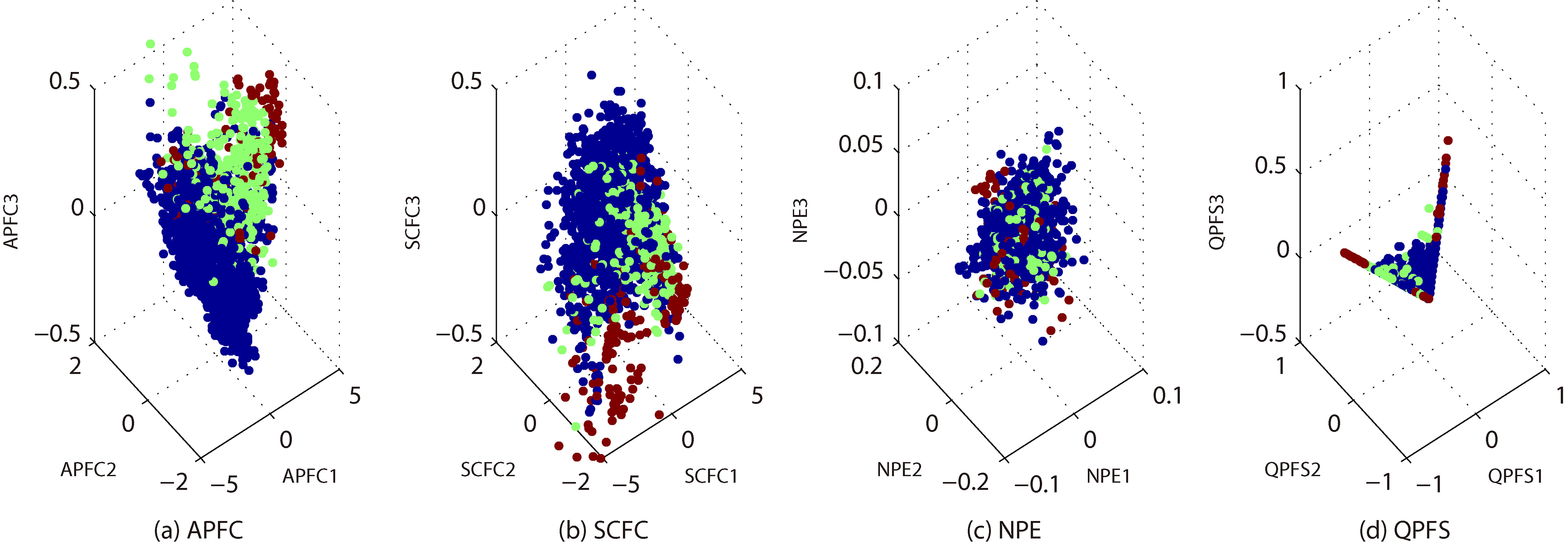
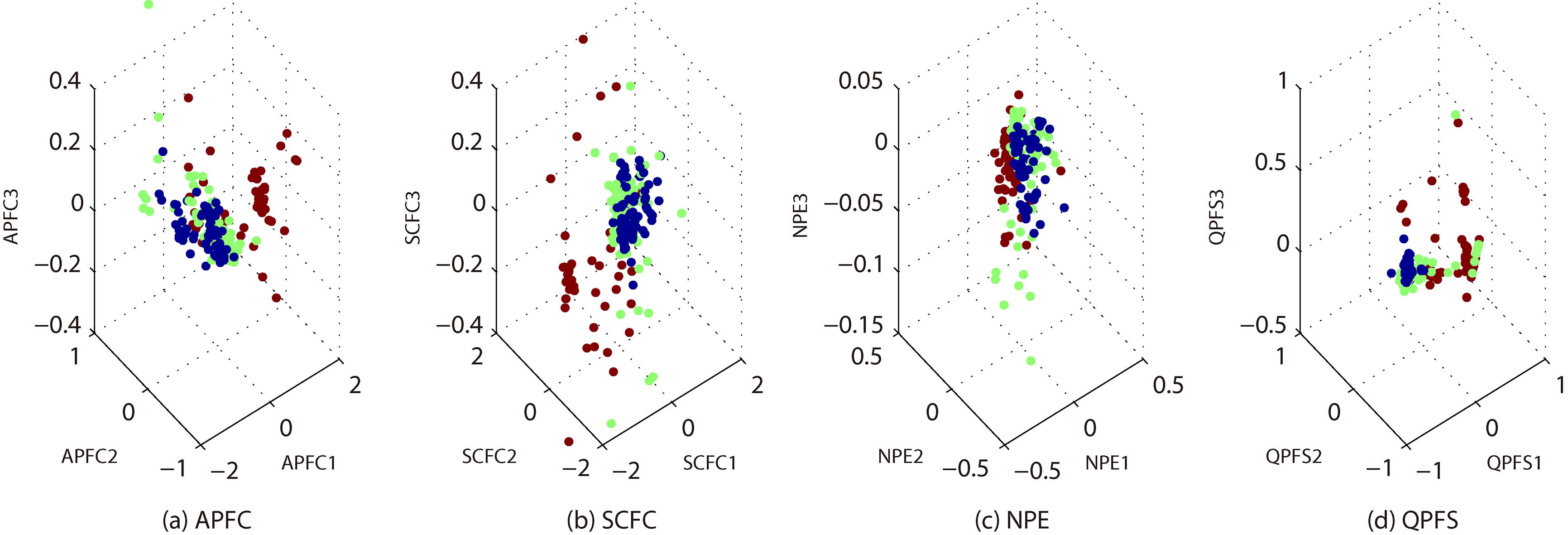
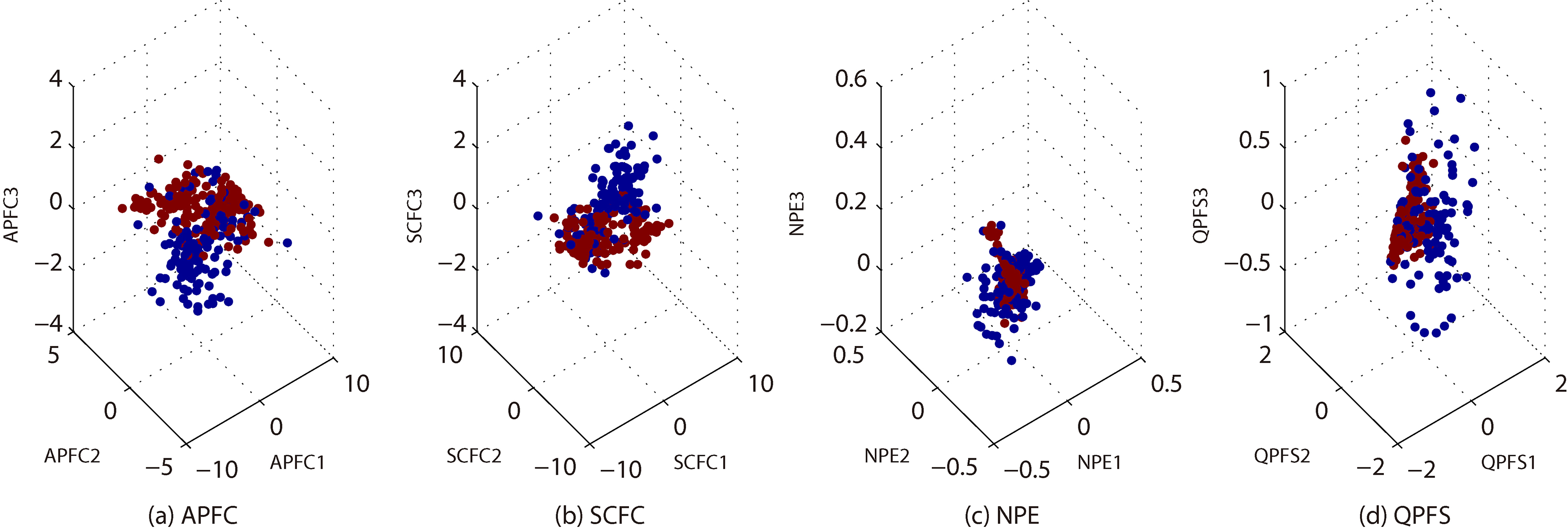
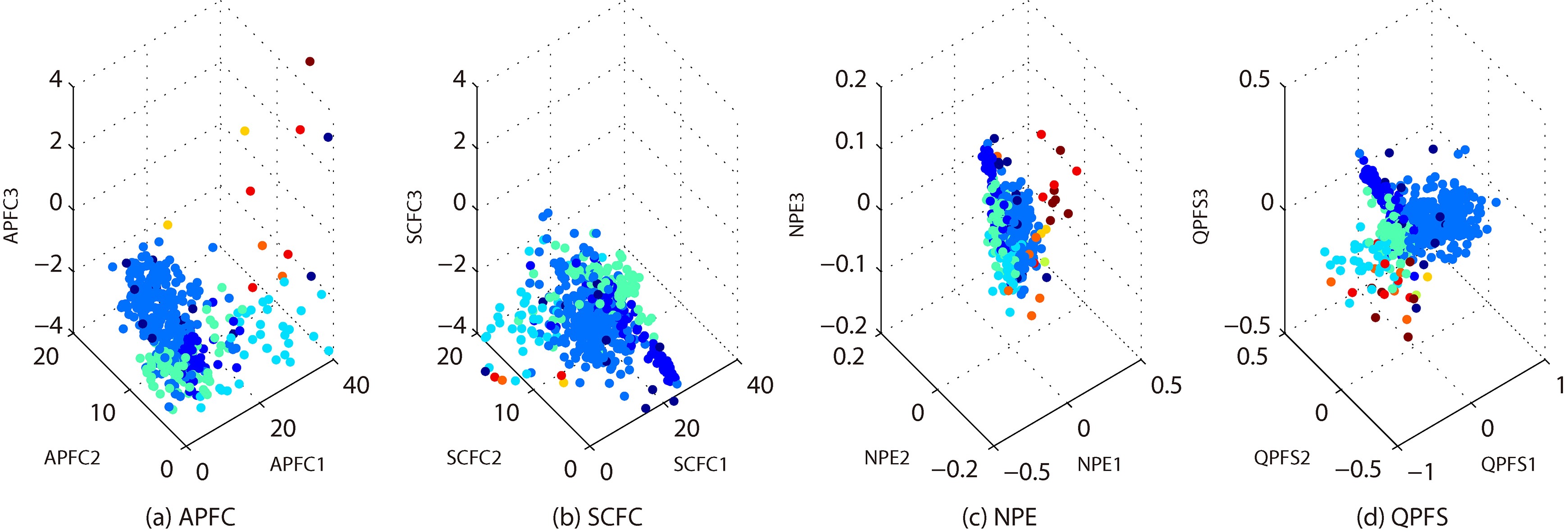
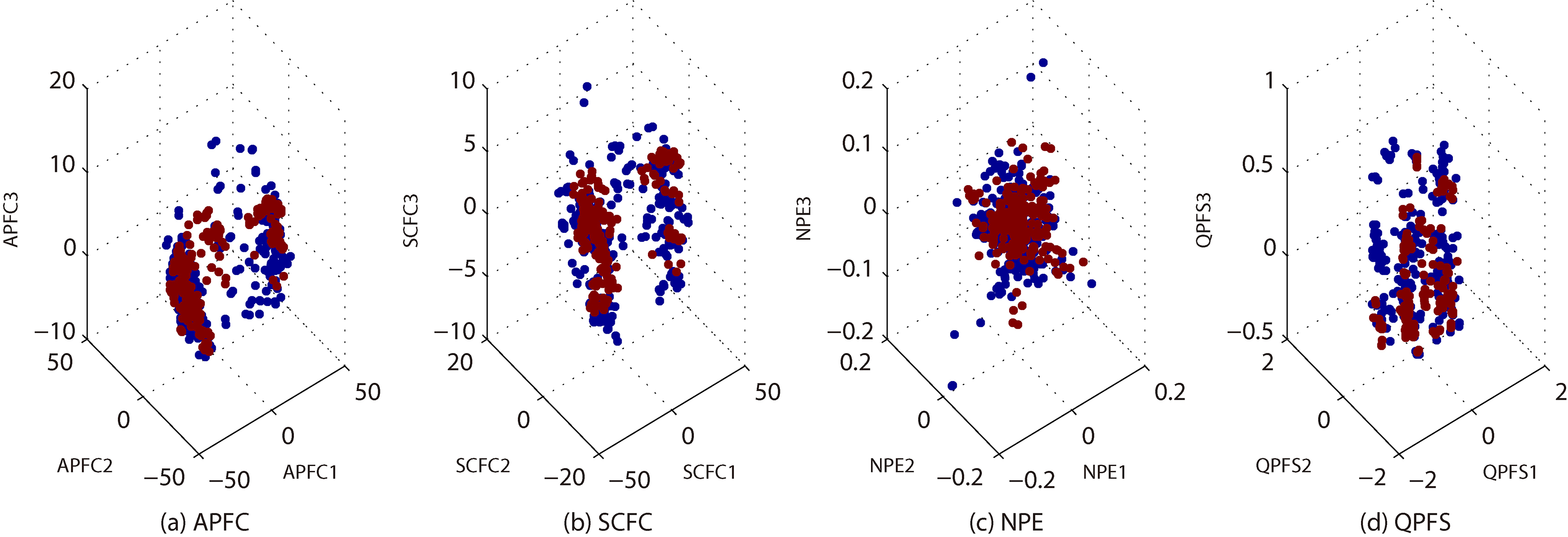
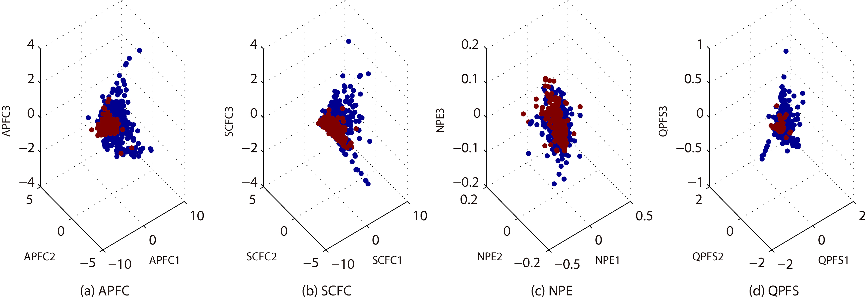
As shown in Table 2, APFC can learn more discriminative features than QPFS, NPE and SCFC. To demonstrate this, we make a number of 3-dimensional embedding illustrations in Figs 2–8. On each dataset, we firstly get the low dimension representation by QPFC, NPE, SCFC and APFC. Secondly, we convert the low dimensional representation into a set of values of linearly uncorrelated variables by principal component analysis (PCA), which is an orthogonal transformation. Finally, we construct a 3-dimensional embedding just from the first three principal components.

Figure 4.

3-dimensional embeddings of GLA.

Figure 5.

3-dimensional embeddings of ION.

In Fig. 2a–d, we show the 3-dimensional embeddings for the reduced BRE by APFC, QPFS, NPE and SCFC. These embeddings belong to 6 classes, represented by different colors. Note that the x-axis, y-axis and z-axis represent the first, second and third principal components, respectively. Likewise, in Figs 3–8 we show more embeddings for CTG, GLA, ION, LRS, MUS and QSA. It can be seen that, APFC embeddings are generally more scattered than NPE and QPFS. It seems that APFC has 3-embeddings similar to SCFC, but it is more effective and efficient (see Tables 2–3).

Figure 6.

3-dimensional embeddings of LRS.

Figure 7.

3-dimensional embeddings of MUS.

Figure 8.

3-dimensional embeddings of QSA.

Table 5

Accs and #dims of APFC with different similarity measure

Data	APFC-P		APFC-NED		APFC-NMI		APFC-Dcor		APFC-MIC
	#dim	Acc	#dim	Acc	#dim	Acc	#dim	Acc	#dim	Acc
ARR	48	76.5487	10	70.1327	60	75.0000	53	75.2212	82	70.1327
BRE	5	66.0377	4	66.9811	4	65.0943	5	60.3774	5	58.4906
CON	13	79.8077	10	78.3654	18	78.3654	15	75.9615	20	76.9231
CTG	3	87.2060	3	83.5372	4	81.7968	5	79.9624	7	86.9238
FTP	12	68.5355	9	58.9408	14	68.1595	10	65.7241	11	67.9797
GLA	3	68.2243	4	58.4112	3	51.4019	4	55.1402	3	50.9346
ION	6	86.3248	5	85.1852	7	85.7550	5	82.9060	10	87.1795
ISO	73	93.0999	50	92.1252	120	94.0105	82	92.6754	140	91.3342
LRS	6	86.6290	8	83.4275	22	88.7006	13	87.5706	18	89.2655
LSV	26	88.0952	17	84.9206	36	84.9206	28	87.3016	41	86.5079
MUS	17	79.4118	16	79.6219	22	80.6723	18	78.1513	22	77.7311
PHI	5	91.6147	6	91.6508	5	90.8820	5	91.3342	7	91.9765
PSS	8	62.5962	7	58.4615	7	62.3077	7	62.8846	7	61.8269
QSA	9	81.2322	7	78.1043	9	83.7915	8	83.7915	11	83.7915

4.5 Effect of different similarity measures

In the above experiments, the Pearson correlation coefficient was taken as similarity between feature associators for APFC. However, different measures of similarity may have an effect on its performance in classification. To show this effect, we select four other measures for comparison, including negative Euclidean distance (NED), normalized mutual information (NMI) [29], distance correlation (Dcor) [30, 31] and maximal information coefficient (MIC) [32].

Table 5 shows the number of extracted features (#dim) and Accs (%) of APFC with different similarity measures on the 14 datasets, where the Accs are the best ones with mixed weightings at $\gamma=$ 0, 0.5, 1. For convenience, we use APFC-P, APFC-NED, APFC-NMI, APFC-Dcor and APFC-MIC to represent different versions of APFC, which may produce different #dim values and Accs. It is easy to see that APFC-P attains both the highest Acc and the lowest #dim on CTG and GLA. Moreover, it reaches the highest Acc on ARR, CON, FTP and LSV. Additionally, APFC-P is in general satisfactory with the rest datasets in terms of Acc and #dim. For example, APFC-NMI attains the highest Acc of 94.0105% with #dim of 120 on ISO, while APFC-P gets a near Acc of 93.0999% with a relatively low #dim of 73. APFC-MIC gets the highest Acc of 91.9765% with #dim of 7 on PHI, while APFC-P gets a near Acc of 91.6147% with a relatively low #dim of 5. Therefore, we can conclude that APFC-P can get better experimental results.

5. Conclusions

In this paper, we have presented an AP clustering algorithm of feature associators, named APFC, for classification problems. It aims at reducing the dimensionality of original features to alleviate the computational cost in the classification procedure. The most important advantage of APFC is to produce robust clusters that are not disturbed by the order of original features, which may lead to different results in other feature clustering algorithms. Moreover, in APFC, the desired number of extracted features need not to be determined by extra parameters or even be provided by users. Additionally, like other feature clustering algorithms, APFC avoids computing the eigenvalues and eigenvectors of covariance matrix which is involved in most feature extraction methods. Finally, compared with QPFS, NPE and SCFC on the 14 UCI datasets, experimental results have demonstrated the effectiveness and efficiency of APFC.

Because of information loss after dimensionality reduction, in experiments APFC may extract new fewer features for a SVM to obtain lower classification accuracy than with all original features. Therefore, it would be future work to improve the performance of APFC in classification with dimensionality reduction.

Footnotes

Acknowledgments

This work was supported in part by the National Natural Science Foundation of China under grant 61175004, the Natural Science Foundation of Beijing Municipality under grant 4112009, the Postdoctoral Science Foundation of China under grant 2015M580952, and the Postdoctoral Research Foundation of Beijing under grant 2016ZZ-24.

References

and Weng

, A survey of image classification methods and techniques for improving classification performance, International Journal of Remote Sensing 28(5) (2007), 823–870.

Kuramochi

and Karypis

, Gene classification using expression profiles: a feasibility study, in: IEEE 2nd International Symposium on Bioinformatics and Bioengineering, IEEE, 2011, pp. 191–200.

Lujan

I.R.

Huerta

Elkan

and Cruz

C.S.

, Quadratic programming feature selection, Journal of Machine Learning Research 11(2) (2010), 1491–1516.

Brown

Pocock

Zhao

M.J.

and Lujn

, Conditional likelihood maximisation: a unifying framework for information theoretic feature selection, Journal of Machine Learning Research 13(1) (2012), 27–66.

Nguyen

X.V.

Chan

Romano

and Bailey

, Effective global approaches for mutual information based feature selection, in: Proceedings of the 20th ACM SIGKDD International Conference on Knowledge Discovery and Data Mining, ACM Press, 2014, pp. 512–521.

Cai

Yan

and Zhang

H.J.

, Neighborhood preserving embedding, in: Proceedings of the 10th IEEE International Conference on Computer Vision, IEEE, 2005, pp. 1208–1213.

Van der Maaten

L.J.P.

Postma

E.O.

and Van den Herik

H.J.

, Dimensionality reduction: a comparative review, Journal of Machine Learning Research 10(1) (2009), 1–41.

Øivind

D.T.

Jain

A.K.

and Taxt

, Feature extraction methods for character recognition-a survey, Pattern Recognition 29(4) (2010), 641–662.

Lewis

D.D.

, Feature selection and feature extraction for text categorization, in: Proceedings of the Workshop on Speech and Natural Language, ACM Press, 2000, pp. 212–217.

10.

Jolliffe

I.T.

, Principal Component Analysis, Springer, New York, 1986.

11.

Belkin

and Niyogi

, Laplacian eigenmaps and spectral techniques for embedding and clustering, Advances in Neural Information Processing Systems 14(6) (2002), 585–591.

12.

Roweis

S.T.

and Saul

L.K.

, Nonlinear dimensionality reduction by locally linear embedding, Science 290(5500) (2000), 2323–2326.

13.

Tenenbaum

J.B.

de Silva

and Langford

J.C.

, A global geometric framework for nonlinear dimensionality reduction, Science 290(500) (2000), 2319–2323.

14.

Baker

L.D.

and McCallum

, Distributional clustering of words for text classification, in: International ACM SIGIR Conference on Research and Development in Information Retrieval ACM Press, 1998, pp. 96–103.

15.

Dhillon

I.S.

Mallela

and Kumar

, A divisive information theoretic feature clustering algorithm for text classification, Journal of Machine Learning Research 3(3) (2003), 1265–1287.

16.

Jiang

J.Y.

Liou

R.J.

and Lee

S.J.

, A fuzzy self-constructing feature clustering algorithm for text classification, IEEE Transactions on Knowledge and Data Engineering 23(3) (2010), 335–349.

17.

R.F.

and Lee

S.J.

, Dimensionality reduction by feature clustering for regression problems, Information Science 299(C) (2015), 42–57.

18.

Pereira

Tishby

and Lee

, Distributional clustering of English words, in: Proceedings of Annual Meeting of the Association for Computational Linguistics, ACM Press, 1994, pp. 183–190.

19.

Frey

B.J.

and Delbert

, Clustering by passing messages between data points, Science 315(5814) (2007), 972–976.

20.

Saul

L.K.

and Roweis

S.T.

, Think globally, fit locally: unsupervised learning of low dimensional manifolds, Journal of Machine Learning Research 4(2) (2003), 119–155.

21.

Pearson

, Notes on regression and inheritance in the case of two parents, Proceedings of the Royal Society of London 58(1895), 240–242.

22.

Dueck

, Affinity propagation: clustering data by passing messages, PhD dissertation, University of Toronto, 2009.

23.

UCI, Machine Learning Repository, http://archive.ics.uci.edu/ml/datasets.html.

24.

Fan

R.E.

Chen

P.H.

and Lin

C.J.

, Working set selection using second order information for training SVM, Journal of Machine Learning Research 6(4) (2005), 1889–1918.

25.

Chang

C.C.

and Lin

C.J.

, LIBSVM-A Library for Support Vector Machines, https://www.csie.ntu.edu.tw/ cjlin/libsvm/.

26.

Nguyen

X.V.

, http://in.mathworks.com/matlabcentral/fileexchange/47129-information-theoretic-feature-selection.

27.

Maaten

L.V.D.

, Matlab Toolbox for Dimensionality Reduction, https://lvdmaaten.github.io/drtoolbox/.

28.

Yan

Zhang

Liu

Yan

Cheng

Fan

Yang

and Chen

, Effective and efficient dimensionality reduction for large-scale and streaming data preprocessing, IEEE Transactions on Knowledge and Data Engineering 18(3) (2006), 320–333.

29.

, Mutual information functions versus correlation functions, Journal of Statistical Physics 60(5–6) (1990), 823–837.

30.

Székely

G.J.

Rizzo

M.L.

and Bakirov

N.K.

, Measuring and testing dependence by correlation of distances, Annals of Statistics 35(6) (2008), 2769–2794.

31.

Székely

G.J.

and Rizzo

M.L.

, Brownian distance covariance, Annals of Applied Statistics 3(4) (2010), 1236–1265.

32.

Reshef

D.N.

Reshef

Y.A.

Finucane

H.K.

Grossman

S.R.

McVean

Turnbaugh

P.J.

Lander

E.S.

Mitzenmacher

and Sabeti

P.C.

, Detecting novel associations in large datasets, Science 334(6062) (2011), 1518–1524.

Feature clustering dimensionality reduction based on affinity propagation

Abstract

Keywords

1. Introduction

2. Background and related work

2.1 Quadratic programming feature selection

4. Experimental results

Table 1 Dataset summary

Table 2 Acc comparison of APFC against other methods

Table 4 Accs of APFC_H, APFC_M, APFC_S on 14 datasets

5. Conclusions

Footnotes

Acknowledgments

References

Table 1
Dataset summary

Table 2
Acc comparison of APFC against other methods

Table 4
Accs of APFC_H, APFC_M, APFC_S on 14 datasets