An innovative method for cardiovascular disease detection based on nonlinear geometric features and feature reduction combination

Abstract

Cardiovascular is arguably the most dominant death cause in the world. Heart functionality can be measured in various ways. Heart sounds are usually inspected in these experiments as they can unveil a variety of heart related diseases. This study tackles the lack of reliable models and high training times on a publicly available dataset. The heart sound set is provided by Physionet consisting of 3153 recordings, from which five seconds were fixed to evaluate to the developed method. In this work, we propose a novel method based on feature reduction combination, using Genetic Algorithm (GA) and Principal Component Analysis (PCA). The authors present eight dominant features in heart sound classification: mean duration of systole interval, the standard deviation of diastole interval, the absolute amplitude ratio of diastole to S2, S1 to systole and S1 to diastole, zero crossings, Centroid to Centroid distance (CCdis) and mean power in the 95–295 Hz range. These reduced features are then optimized respectively with two straightforward classification algorithms weighted k-NN with a lower-dimensional feature space and Linear SVM that uses a linear combination of all features to create a robust model, acquiring up to 98.15% accuracy, holding the best stats in the heart sound classification on a largely used dataset. According to the experiments done in this study, the developed method can be further explored for real world heart sound assessments.

Keywords

Heart sounds classification feature selection dimensionality reduction optimization

1. Introduction

Nowadays, Cardiovascular disease has become one of the main causes of all diseases & death worldwide. Based on the WHO report, in 2012, about 17.5 million people died from cardiovascular disease that includes about one-third of the global mortality rate. The first step in assessing a heart system in the clinical condition is performing a physical experiment. Heart sounds are the most crucial part of physical experiments & they can recognize heart diseases as well as heart failure, arrhythmias, heart valve failure, etc. Also, heart sounds are one of the most significant signs in early diagnosis of all diseases which can be used in diagnostic experiments. Heart sounds has been used frequently to evaluate heart rate and its functionality [1]. In 1997, Liang et al. [2], proposed a heart sound segmentation algorithm, the authors studied 37 subjects containing normal and abnormal cases. The methodology was based on normalized average Shannon energy of phonocardiogram (PCG) signals, which reduces low frequency noises, and finally based on a threshold, peaks are determined as the heart sounds. In another work [3], they experimented with 77 cases using discrete wavelet decomposition (DWT) as a feature to segment heart sounds into four parts: S1, Systole, S2 and Diastole. Rajan et al. [4], worked on 42 cases containing normal and pathological participants using signal energy and singular value decomposition (SVD) derived from morlet wavelets to identify important activities as useful features for segmenting PCG signals. Sepehri et al. [5], studied 60 pediatric subjects, the study used short-time spectral energy and autoregressive parameters as the distinct features and selected Multi-Layer Perceptron (MLP) as the most effective classifier. Schmidt et al. [6] used duration-dependent hidden Markov models (DHMM) for segmenting heart sounds of 73 subjects. In 2012, Naseri et al. [7] used a combination of frequency-based and amplitude-based features, extracted from sliding windows. The dataset consisted of 52 minute recordings of patients of divergent heart abnormalities. Sun et al. [8], worked on 121 subjects, including 45 normal and 76 abnormal cases. They utilized the attributes of Hilbert transform (HT) to detect the moment segmentation and peak points of heart sounds by using zero-crossing methods. In 2016, Tang et al. [9] introduced clustering to compress of the PCG signals which reduces storage capacity in the recording system, the study acquired varying compression ratios from 20 to 149 times. Dominguez et al. [10], used the a neuromorphic auditory sensor to analyze audio information in frequency boundaries in real time. After that sonograms are created from the frequency information, and fed to AlexNet for classification. In 2018, Latif et al. [11] proposed recurrent neural networks (RNN) to simplify real-time heart rate monitoring of normal and abnormal patients. Garg et al. [12] developed cross recurrence quantification analysis (CRQA), analyzing the harmony between synchronized ECG and PCG signals. In 2020, Krishnan et al. [13], worked on 1081 PCG records with frequency rates of 500 HZ, discrimination was done using one-dimensional convolutional neural networks and feed forward neural networks performed on unsegmented PCG signals.

2. Materials and methods

2.1 Database

The Data used in this study is provided in an open-source database by Physionet from the 2016 challenge. Dataset consists of 3153 recordings, which contains both normal and noisy recordings with such as stethoscope, talking or movement artifacts. Seven hundred and sixty-five of the patients were labeled as pathological. Recordings had a sampling rate of 2000 Hz, and the duration varied between 5 to 120 seconds. More details on the database are provided by Li et al. [14]. In this work, the length of all the analyzed recordings was fixed to 5 seconds to speed up the operation time of the algorithm and also use the same amount of information for each particular subject to prevent overfitting. All the computations were done using MATLAB.

Figure 1.

The resulting Markov chain in PCG segmentation using HMMs. Four horizontal steps are related to the consecutive heart sounds, creating a complete cardiac cycle.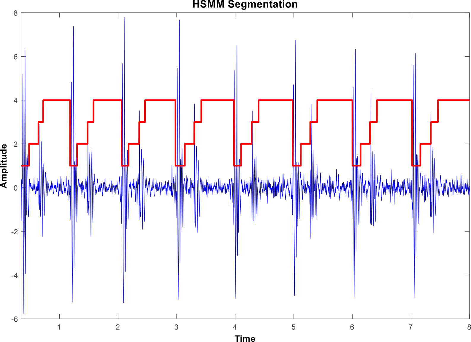

2.2 Preprocessing

Preprocessing includes having all the recordings resampled to 1000 Hz for processing purposes and a Butterworth bandpass filter of second-order (50–800 Hz), normalization was done to reduce noise effects. Schmidt’s spike removal algorithm was also employed to further make the data suitable for processing. Secondly, state-of-art [15] Springer’s hidden semi-Markov model (HSMM) based segmentation algorithm was applied to each recording to extract the individual heart sounds. Hidden semi-Markov models have an unobservable semi-Markov chain indicating the probability to change state based on the time passed in the current state. Assuming that there are $Q$ hidden states:

$\displaystyle Q=\{q_{i}\},i=1,2,3,\ldots,$ (1)

where $q_{i}$ indicates the number of unobservable states. The transition probabilities are calculated as follows:

$\displaystyle{A=a}_{ij}=P(q_{j}(t+1)|q_{i}(t))$ (2)

where $q_{i}$ denotes the current state and $q_{j}$ shows the next state, with $t$ demonstrating time, the Transition probability $a_{ij}$ emits the probability that the next state is $q_{j}$ given that the existing state is $q_{i}$ . Observations, necessary for prediction of hidden states are defined as:

$\displaystyle O=\{o_{k}\},k=1,2,3,\ldots,M$ (3)

where $o_{k}$ is a set of observations with an underlying hidden state to be found. Emission probabilities can be computed having the information in hand:

$\displaystyle B=b_{ij}=b_{i}(o_{k})=P(o_{k}|q_{i})$ (4)

where $B$ is the probability of observing $o_{k}$ when the given state is $q_{i}$ . Initial state probabilities can be calculated as follows:

$\displaystyle\prod=p_{i}=P(q_{i}(t=1))$ (5)

where $\Pi$ is the probability of seeing the state $q_{i}$ when $t=1$ . In this case, the semi-Markov chain is the details on the subject’s current heart sound state, which is composed of the four heart sounds described earlier. This information allows us to analyze different heart sounds in divergent heartbeats individually. Figure 1 shows the resulting Markov chain in PCG segmentation using HMMs. Where each step shows a successfully discriminated heart sound, composing of S1, Systole, S2 ad Diastole respectively, with each four step cycle denoting a heart beat.

2.3 Feature extraction

In this phase of the work, 61 features are extracted from three different domains trying to represent the data in an elaborate manner. These domains include time-domain, frequency-domain, and time-frequency domain.

Figure 2.

CCdis calculation procedure in abnormal patients.

2.3.1 Time-domain features

Time-domain features have proven essential because of having the ability to recognize anomalies in heart sounds, including durations, higher-order spectra, and self-similarity techniques. Our time-domain features include 36 features consisting of state durations derived from the semi-Markov chain, which involve mean and standard deviations of heartbeat duration (RR), S1, S2, systole, and diastole intervals. Other Features include mean and standard deviations of interval duration ratios of systole to RR, diastole to RR, and systole to diastole. These features were also included in the sample entry provided by Physionet. We also added some amplitude ratio properties to enhance these 16 features. These features were used by Potes et al. [16] the 1 ${}^{\text{st}}$ entry in the Physionet 2016 challenge: mean amplitude ratio of diastole to systole, diastole to S2, S1 to systole, S1 to S2, S1 to diastole and systole to S2 in each heartbeat, which adds up to 22 features. Hurst’s exponent was also calculated for the whole recording in each individual. Hurst’s exponent shows long-term correlations in a signal based on the decrease rate of autocorrelation function when the lag is slowly increased. Hurst’s exponent is related to fractal dimension regarding this formula:

$\displaystyle Dim=2-H$ (6)

where the dimensionality of the time-series denoted by $D i m$ varies between $1<Dim<2$ , and Hurst’s exponent represented by $H$ scales between 0 and 1, the higher the $H$ value, the lower the fractal dimension, resulting in a smooth and less complex signal. The opposite stands for time-series with a greater fractal dimension. Hurst’s exponent is usually calculated using the following formula:

$\displaystyle H_{q}=H(q)$ (7)

Is measured for a time series:

$\displaystyle x(t),t=1,2,3,\ldots$ (8)

If $S_{q}$ is the scaled time-series in different lags. For each lag ( $\tau$ ), $S_{q}(\tau)$ is calculated:

$\displaystyle S_{q}=\{|x(t+\tau)-x(t)|^{q}\}_{t}\sim\tau^{qH(q)}$ (9)

where $q>0$ (usually 1 or 2), and the lag is always smaller than the greatest scale in the time-series. An exponent value bigger than 0.5 indicates persistent behavior, and exponent values less than 0.5 show anti-persistent behavior. $H_{q}$ values of 0.5 and 0 are considered to be Brownian noise and Pink noise, respectively. Other time-domain features include mean zero crossings rate in each RR interval [17], and heartbeat CCdis (Centroid to Centroid distance) previously introduced by the authors [18], which first decomposes the signal into a series of overlapping triangles (13% overlap in this study) and then proceeds to calculate the distance between triangle centroids, in the last step mean distance changes in consecutive triangles are computed. The formula for CCdis calculation includes, initially finding centroid coordinates using the following formula.

Figure 3.

CCdis calculation procedure in normal participants.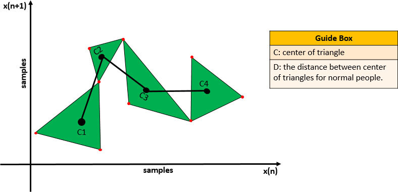

For a time-series:

$\displaystyle x(t),t=1,2,3,\ldots$ (10) $\displaystyle\text{centroidX}=\frac{x_{t}+x_{t+2}+x_{t+4}}{3}$ (11) $\displaystyle\text{centroidY}=\frac{x_{t+1}+x_{t+3}+x_{t+5}}{3}$ (12)

where centroidX and centroidY demonstrate each triangle centroid’s $x$ and $y$ coordinates, respectively. After that, the distance among two consecutive triangles is measured as follows:

$\displaystyle D=\sqrt{{(x_{2}-x_{1})}^{2}+{(y_{2}-y_{1})}^{2}}$ (13)

with $(x_{2},y_{2})$ and $(x_{1},y_{1})$ showing the coordinates of each consecutive triangle, and $D$ the distance between the two centroids.

Figures 2 and 3 show the CCdis calculation procedure in abnormal and normal patients, respectively.

Higher-order spectra [16, 17, 9] were also extracted for every heartbeat: mean and standard deviation of kurtosis in the S1 interval, the standard deviation of skewness in S1 interval, mean and standard deviation of kurtosis in systole interval, mean values of kurtosis and skewness in the S2 interval and mean and standard deviation of kurtosis and skewness in the diastole interval. Kurtosis and Skewness refer to ‘tailedness’ and asymmetry in the probability distribution of a variable around its mean, respectively.

2.3.2 Frequency-domain features

Frequency-domain features are widely used for heart sound classification as heart murmurs can be identified by their frequency components [19, 20, 21, 22]. In this work, initially, power spectrum was calculated for each individual using Welch’s averaged periodogram technique, in this case, the method’s frequency resolution reduction seems a fair trade because of the ability of this technique to improve the results in noisy recordings which is an important issue with the dataset in hand, which has recordings under different conditions. In Welch’s method, first, each signal is turned into overlapping segments then a window function is applied, after that discrete Fourier transform (DFT) is performed to measure a periodogram for each segment, in the end, the averaged periodograms from all segments result in the final power elements of the signal. The parameters used in this method were: Hamming window, 50% overlap as default, in this study mean powers of the specific frequency bands in the ranges: 1–95 Hz, 95–295 Hz, 295–485 Hz, 485–585 Hz, and 585–685 Hz were used concluding 5 frequency-domain features.

2.3.3 Time-frequency features

Twenty Time-Frequency features extracted include generalized Hurst’s exponent applied to wavelet packet decomposition [19, 23, 24, 41] (WPD) coefficients with a depth of 3, the mother wavelet was also selected to be Daubechies 4 [24, 34]. In WPD signal goes through low-pass and high-pass filters simultaneously, resulting in approximate and detail coefficients, respectively (DWT). Equation (14) demonstrates the formula for computing DWT of a time-series:

$\displaystyle c[i]=(x*h)[i]=\sum^{\infty}_{k=-\infty}{x[k]h[n-k]}$ (14)

where the time-series $x$ is passed through low and high pass filters that have an impulse response $h$ . In our method, all of the coefficients in the third level of the tree were used, resulting in 7 features. Hurst’s Exponent was chosen based on its superior discrimination rate compared to frequently used features such as Sample entropy, log energy, and Shannon’s entropy [9, 17, 25]. Furthermore, Mel frequency Cepstral coefficients (MFCC) were extracted for each heartbeat in each subject. MFCCs are also very popular in heart sound processing [9, 11, 16, 25, 26, 27]. In MFCC, the signal is shown in a nonlinear Mel scale after being shifted to the Cepstral representation, which composes of performing the DFT, then applying triangular windows to get the spectrum in the Mel scale, after that the discrete cosine transform is performed on the log power of each Mel frequency. Equation (15) shows the procedure to convert the frequency to the Mel scale:

$\displaystyle M(f)=1125\ln\left(1+\frac{f}{700}\right)$ (15)

with $f$ showing the desired frequency to transform. Following formula demonstrates the DFT involved in the MFCC steps:

$\displaystyle X_{i}(k)=\sum^{N}_{n=1}{x_{i}}h(n)e^{-\frac{j2\pi kn}{N}},∼{}1% \leqslant k\leqslant M$ (16)

Assuming that the time-series is $x_{i}$ , $h(n)$ being an $N$ sized window and $M$ the length of the DFT. For all of the frames (shown by $i$ ) power spectrum is calculated using the following formula:

$\displaystyle S_{i}(k)=\frac{1}{N}{|X_{i}(k)|}^{2}$ (17)

where $S_{i}(k)$ is known as the periodogram estimate. Mean values for each coefficient were calculated over all of the heartbeats resulting in 13 MFCC features.

2.4 Feature reduction

In the feature reduction procedure, in order to overcome the curse of dimensionality and decrease the time required to train the model, feature reduction and selection [30, 31, 32] methods are performed. Several techniques were examined in this study, namely genetic algorithm (GA) [39, 40], feature ranking, and principal component analysis (PCA) [22, 37, 38]. Feature ranking was evaluated based on $t$ -values and entropies. Information mutuality was also considered using the CCWeighting and NWeighting features in MATLAB. PCA performs an orthogonal transformation on the features to reduce dimensionality as well as creating a space of linearly uncorrelated components. As an example for the first principal component, at first, the data needs to be centered then a least-squares sense line is fit to the data so that the ratio of the more contributing feature is higher, the square-root of distance from the line to the data points (so-called Eigenvalue) is the singular value for principal component one. The four first principal components were used as classifier inputs. GA is built on Darwin’s natural evolution theory. In computer science, it’s mostly used to solve searching and optimization problems. Figure 4 shows the steps in a simple genetic algorithm.

Figure 4.

Simplified diagram of a typical genetic algorithm lifecycle.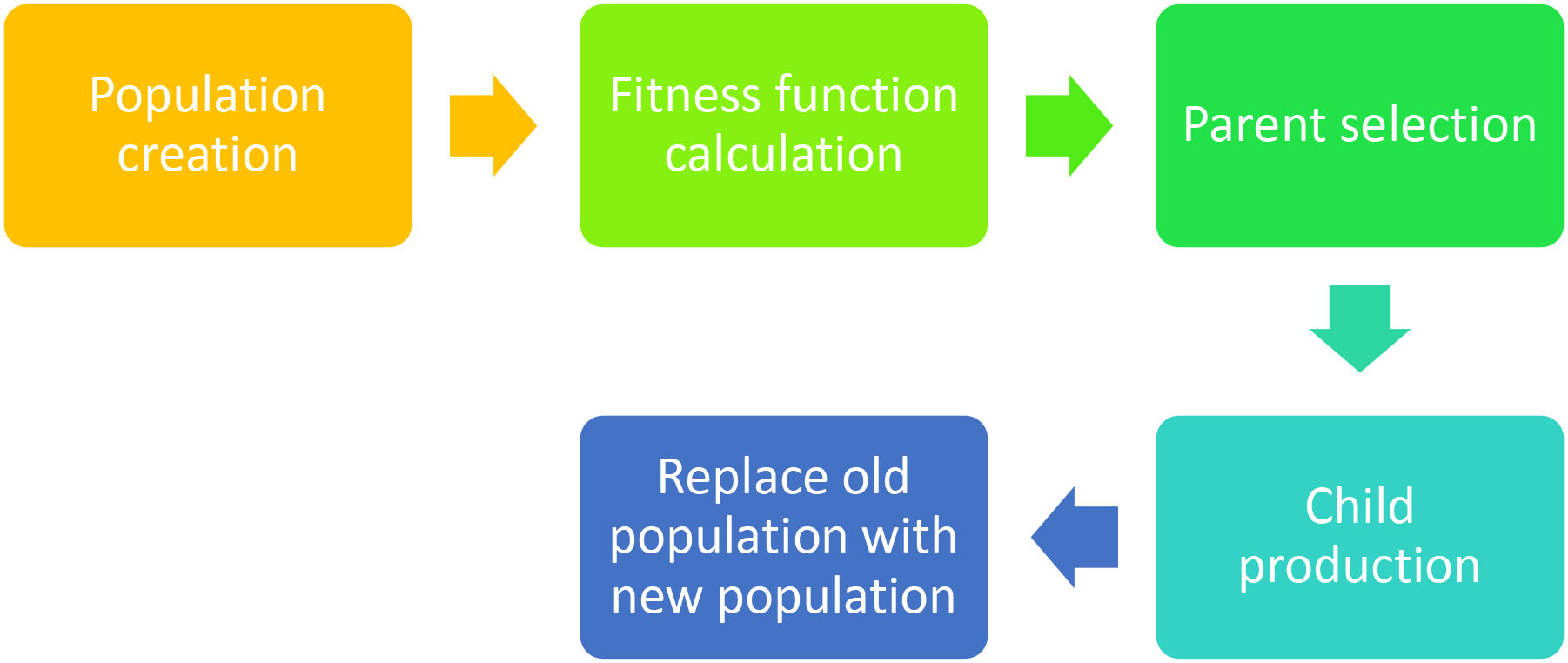

In the GA, initially a population of $N$ elements is made randomly. Then the fitness function is calculated for each of the population members. After that according to the number of generations or the set number for fitness, this repetitive iteration will take place, choosing several parents based on the probabilities from fitness (selection), producing a ‘child’ based on the parents (crossover), lastly based on the mutation percentage some changes may happen to the ‘child’ to keep the variety, in the end, the ‘child’ is added to the population after $N$ steps the new population replaces the older one. This loop will keep going until the criteria are met. Crossover and mutation rates of 0.8 and 0.01 were chosen respectively for the algorithm. According to GA, these 8 features are sufficient to represent the data: mean duration of systole interval, the standard deviation of diastole interval, the absolute amplitude ratio of diastole to S2, S1 to systole, and S1 to diastole, zero crossings, CCdis and mean power in the 95–295 Hz range.

2.5 Classification

Extracted features and reduced spaces derived from the feature space and feature reduction methods were examined to find an appropriate classification method in the classification step. Several popular classification techniques were inspected in this work, such as Artificial neural networks (ANN), Probabilistic neural networks (PNN), Naive Bayes (NB), Adaptive Boosting (AdaBoost), k-nearest neighbors (k-NN), decision tree, linear discriminant analysis, self-organizing fuzzy logic introduced recently by Xiaowei et al. [33], and support vector machines (SVM). An explanation for the best working techniques in this study follows below.

2.5.1 Weighted k-NN

K-nearest neighbor is a lazy machine learning algorithm frequently used in classification problems [34, 35], it’s often desired because of simplicity and also the upside of not making any assumptions about the data, being lazy means that k-NN does not need training and simply makes decisions based on distance compared to existing samples in the feature space. According to $k$ value, the number of neighbors needed to label a particular recording is determined. In this work, the k-NN uses Minkowski distance with an order of 1.5, and inverse distance weighs $k=$ 3 and the $k$ - $d$ tree as the nearest neighbor searching method. Minkowski distance between two points with $i$ dimensions can be defined using the following equation:

$\displaystyle D=\left(\sum^{n}_{i=1}|x_{i}-y_{i}|^{p}\right)^{\frac{1}{p}}$ (18)

where $p$ is the order and is always $p\geqslant 1$ . $p$ values of 1 or 2 result correspond to Manhattan distance and Euclidean distance, respectively. Lastly, a $p$ value of $\infty$ results in Chebyshev distance. the $k$ - $d$ tree is used for space-partitioning and arranging data in $k$ -dimensional spaces. Feature vector scaling was also done to enhance the performance of the classifier.

2.5.2 Linear SVM

SVMs are one of the most used supervised learning techniques for classification and regression [9, 20, 22, 24, 26, 36]. Linear SVM tries to separate the data by finding a maximum-margin hyperplane. It is quite obvious that linear SVM reduces model complexity compared to nonlinear kernel SVMs. In a dataset consisting of $n$ points:

$\displaystyle(\vec{x}_{1}\cdot y_{1})\ldots(\vec{x}_{n}\cdot y_{n})$ (19)

where $y_{i}$ is the class labels containing $-$ 1 and 1, and $x_{i}$ is the feature vector, each containing a number of observations form a particular subject. The hyperplane is written as follows:

$\displaystyle\vec{\omega}\cdot\vec{x}-b=0$ (20)

where $\vec{\omega}$ is the normal vector perpendicular to the hyperplane. The SVM used in this paper worked based on Quadratic programming.

Figure 5 shows the decision boundary in support vector machines.

Figure 5.

Decision boundary in support vector machines.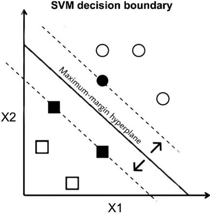

2.6 Model evaluation

In this stage, 10-fold-cross-validation was performed to measure the reliability of the proposed classification method. Cross-validation is used to find out how well the classification method performs when the test data is unseen. Thus the performance measurement on the whole data seems necessary. In this technique, data is randomly divided into 10 groups, then the classifier is trained using 9 folds, and the testing is done on the remaining fold. This process continues so that all of the 10 folds are once used as testing data, then the average value over these sequences is reported as the final confusion matrix of the classifier. The cross-validation was done several times to ensure that the results are well-grounded. Finally, based on the confusion matrix, sensitivity, specificity, accuracy, and F1 score are calculated for the model.

$\displaystyle\text{Sensitivity}=\frac{\textit{TP}}{\textit{TP}+\textit{FN}}% \times 100$ (21) $\displaystyle\text{Specificity}=\frac{\textit{TN}}{\textit{TN}+\textit{FP}}% \times 100$ (22) $\displaystyle\text{Accuracy}=\frac{\text{Sensitivity}+\text{Specificity}}{2}$ (23) $\displaystyle\text{F1 score}=\frac{2\textit{TP}}{(2\textit{TP}+\textit{FP}+% \textit{FN})}\times 100.$ (24)

where TP, TN, FP and FN sand for true positive, true negative, false positive, and false negative, respectively.

Figure 6 shows the block diagram of the proposed method.

3. Results

3.1 Statistical analysis

Student’s $t$ -test was performed to prove the usefulness of the features. This method is a statistical test that investigates the possibility of a significant difference in the means of two uncorrelated groups, where the null hypothesis is that the groups have the same means. The technique uses variance to make this decision. The significance level $\alpha$ determines the acceptance or rejection of the null hypothesis and is usually set at 0.05. A $t$ -test is defined by two important parameters $p$ and $t$ values. Where $p$ values lower than 0.05 demonstrate statistical significance. As $t$ value represents the amount of significance. Equation (25) shows the procedure to calculate the $t$ stat:

$\displaystyle t=\frac{\mu_{a}-\mu_{n}}{\sqrt{\frac{SS^{2}_{a}}{N}+\frac{SS^{2}% _{n}}{M}}}$ (25)

where $\mu_{a}$ , $\mu_{n}$ indicate means in each group, $SS_{a}$ and $SS_{b}$ show sample standard deviations and $N$ and, $M$ represent the size of each group.

3.2 Time-domain results

Table 1 shows the average values from time-domain features between the groups. Based on interval features, The abnormal group had relatively longer RR segments, resulting in longer heart sounds in general (S1, S2, Systole, Diastole) although with relatively larger deviations. Among the more discriminate features: Amplitude ratios suggest that the abnormal group exhibits a higher relative absolute amplitude with respect to the normal group. Hurst’s exponent results indicate that the abnormal group show more complex behavior compared to the normal group due to lower exponent value. Also, based on CCdis values, the abnormal group demonstrated greater average distance among their structure. Higher-order statistics also showed relatively good discrimination rates as they were also used in heart sound segmentation algorithms resulting in a reliable demonstration of heart sounds. With the abnormal group demonstrating higher mean and deviation in kurtosis of S1, Systole and Diastole, and greater standard deviation in the skewness of the S1 segment, and the normal group showed relatively higher mean kurtosis in the S2 segment. Zero crossing rates were also greater in the abnormal group, showing the fluctuations in heart sounds with a larger standard deviation.

Table 1
$p$ -values and properties of the selected time-domain features. Containing mean and standard deviations for each group, followed up by the $p$ -value

Feature	Abnormal group		Normal group		$p$ -value
	Mean $\pm$	Std	Mean $\pm$	Std
M_RR	2102.4 $\pm$	789.0812	1865.7 $\pm$	343.7945	0.0795
Sd_RR	137.2222 $\pm$	88.9245	82.5185 $\pm$	59.1675	0.0052
M_IntS1	265.3333 $\pm$	25.9911	262.5926 $\pm$	22.0720	0.3390
Sd_IntS1	37.4444 $\pm$	15.7488	26.5185 $\pm$	14.4631	0.0057
M_IntS2	224.1481 $\pm$	23.5433	217.2963 $\pm$	21.7818	0.1360
Sd_IntS2	32.5926 $\pm$	14.8538	23.7778 $\pm$	12.9684	0.0121
M_IntSys	391.2593 $\pm$	247.8381	337.7037 $\pm$	64.9288	0.1412
Sd_IntSys	47.2222 $\pm$	25.8863	30.3704 $\pm$	18.8499	0.0043
M_IntDia	1215.3 $\pm$	692.4944	1045.2 $\pm$	272.2141	0.1201
Sd_IntDia	102.5926 $\pm$	99.5784	60.7037 $\pm$	33.7591	0.0217
M_Ratio_SysRR	19.7637 $\pm$	7.9646	18.3200 $\pm$	2.3077	0.1849
Sd_Ratio_SysRR	1.7519 $\pm$	0.9635	1.3754 $\pm$	0.7344	0.0562
M_Ratio_DiaRR	54.2520 $\pm$	13.0860	55.2196 $\pm$	5.2497	0.3618
Sd_Ratio_DiaRR	2.5583 $\pm$	1.4573	1.9974 $\pm$	1.3167	0.0719
M_Ratio_SysDia	41.7215 $\pm$	23.7874	33.8614 $\pm$	7.1649	0.0531
Sd_Ratio_SysDia	4.8862 $\pm$	3.6677	3.3715 $\pm$	2.6857	0.0447
M_Amp_Ratio_DiaSys	219.1689 $\pm$	1076.0	116.8430 $\pm$	348.3077	0.0877
M_Amp_Ratio_DiaS2	37.6787 $\pm$	102.6693	240.0371 $\pm$	764.9429	0.0148
M_Amp_Ratio_S1Sys	2.7369 $\pm$	1.3897	4.7040 $\pm$	3.1583	0.0113
M_Amp_Ratio_S1S2	3.1357 $\pm$	3.9966	3.0145 $\pm$	3.4634	0.0675
M_Amp_Ratio_S1Dia	1.4395 $\pm$	1.1222	1.6728 $\pm$	1.3091	0.0622
M_Amp_Ratio_SysS2	3.7894 $\pm$	13.2198	0.8830 $\pm$	1.1633	0.0574
Hurst’s exponent	0.4901 $\pm$	0.1220	0.5986 $\pm$	0.0772	1.5769e-05
Zero crossings	131.3247 $\pm$	87.5106	89.6457 $\pm$	43.6924	0.0156
CCdis	0.3887 $\pm$	0.1029	0.2806 $\pm$	0.0600	9.186e-06
M_kurtosis_S1	4.6116 $\pm$	1.6831	3.9566 $\pm$	1.1999	0.0382
Sd_kurtosis_S1	1.7728 $\pm$	1.5265	1.1006 $\pm$	1.4204	0.0041
Sd_skewness_S1	0.5710 $\pm$	0.4269	0.4268 $\pm$	0.4819	0.0071
M_kurtosis_Sys	6.5208 $\pm$	5.2439	5.6230 $\pm$	2.7368	0.0205
Sd_kurtosis_Sys	4.9456 $\pm$	6.7456	4.3273 $\pm$	3.9746	0.0330
M_kurtosis_S2	5.0274 $\pm$	1.4537	5.6395 $\pm$	2.5434	0.1066
M_skewness_S2	0.2029 $\pm$	0.3757	0.2015 $\pm$	0.6345	0.0721
M_kurtosis_Dia	12.6824 $\pm$	9.5954	10.8127 $\pm$	7.1841	0.0731
Sd_kurtosis_Dia	9.7966 $\pm$	11.9986	9.5398 $\pm$	13.7925	0.0698
M_skewness_Dia	0.0371 $\pm$	0.4901	0.1681 $\pm$	0.8080	0.1545
Sd_skewness_Dia	0.8661 $\pm$	0.6636	1.0174 $\pm$	0.8316	0.1680

Figure 6.

A simple block diagram for the developed technique.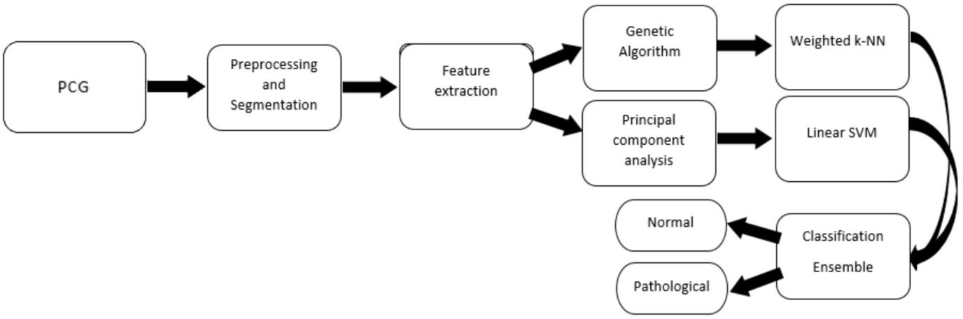

Table 2

$p$ -values and properties of the selected frequency domain features, the abnormal group clearly demonstrates more high frequency sounds

Feature	Abnormal group		Normal group		$p$ -value
	Mean $\pm$	Std	Mean $\pm$	Std
M_Power_1-95 Hz	378.2309 $\pm$	166.4613	498.7290 $\pm$	124.5176	0.0020
M_Power_95-295 Hz	211.1371 $\pm$	140.2196	91.9702 $\pm$	74.7237	1.3966e-04
M_Power_295-485 Hz	8.1267 $\pm$	17.8722	0.8351 $\pm$	1.0751	0.0196
M_Power_485-585 Hz	5.1066 $\pm$	14.1302	0.5022 $\pm$	0.7329	0.0484
M_Power_585-685 Hz	3.6665 $\pm$	12.8032	0.5015 $\pm$	0.9820	0.1030

Table 3

$p$ -values and properties of the selected time-frequency features

Feature	Abnormal group		Normal group		$p$ -value
	Mean $\pm$	Std	Mean $\pm$	Std
Hurst_WPD_3.0	0.0147 $\pm$	0.0156	0.0212 $\pm$	0.0178	0.0423
Hurst_WPD_3.1	0.0307 $\pm$	0.0257	0.0435 $\pm$	0.0314	0.0532
Hurst_WPD_3.2	0.0255 $\pm$	0.0287	0.0429 $\pm$	0.0346	0.0247
Hurst_WPD_3.3	0.0885 $\pm$	0.0486	0.0295 $\pm$	0.0587	9.1949e-05
Hurst_WPD_3.4	0.0198 $\pm$	0.0220	0.0267 $\pm$	0.0268	0.1537
Hurst_WPD_3.5	0.0566 $\pm$	0.0390	0.0338 $\pm$	0.0300	0.0099
Hurst_WPD_3.6	0.0563 $\pm$	0.0406	0.0071 $\pm$	0.0505	1.2117e-04
Hurst_WPD_3.7	0.0013 $\pm$	0.0218	0.0161 $\pm$	0.0267	0.0057
M_Mel_Logenergy	$-$ 15.6974 $\pm$	0.7086	$-$ 15.1441 $\pm$	1.4964	0.442
M_MelScale1	0.9766 $\pm$	0.2914	0.8009 $\pm$	0.2713	0.0129
M_MelScale2	0.3136 $\pm$	0.1186	0.2380 $\pm$	0.0827	0.0045
M_MelScale3	0.1569 $\pm$	0.0845	0.0735 $\pm$	0.1517	0.0079
M_MelScale4	0.1866 $\pm$	0.0798	0.0560 $\pm$	0.0796	8.9654e-08
M_MelScale5	$-$ 0.0735 $\pm$	0.1007	0.0208 $\pm$	0.0505	3.2067e-05
M_MelScale6	$-$ 0.0585 $\pm$	0.0803	0.0294 $\pm$	0.0497	6.1346e-06
M_MelScale7	0.0797 $\pm$	0.0490	0.0312 $\pm$	0.0205	8.2267e-06
M_MelScale8	0.0032 $\pm$	0.0209	0.0175 $\pm$	0.0194	0.0060
M_MelScale9	0.0346 $\pm$	0.0272	0.0078 $\pm$	0.0141	1.5924e-05
M_MelScale10	$-$ 0.0859 $\pm$	0.0586	$-$ 0.0123 $\pm$	0.0387	7.0206e-07
M_MelScale11	0.0600 $\pm$	0.3708	0.2694 $\pm$	0.1174	24654e-05
M_MelScale12	0.01897 $\pm$	0.0423	0.03247 $\pm$	0.0197	1.6222e-06

3.3 Frequency-domain results

Table 2 shows the mean digits resulting from frequency-domain features in each group. Interesting power relations were observed, the abnormal group showed dominant mean powers up to frequency band of 95 Hz indicating lower murmur frequencies in normal sounds, in oscillations higher than 95 Hz, the abnormal group demonstrated greater mean powers. The difference above was the particular reason to select these bands based on $p$ -values.

3.4 Time-frequency results

Table 3 shows the mean values in time-frequency features between the two groups. WPD features suggest that 3.3 and 3.6 coefficients are the most discriminate frequencies; these coefficients correspond to frequency bands of (331.25–425) Hz and (706.25–800) Hz, respectively. Also, all MFCC features showed a superior discrimination rate compared to other features, according to $p$ -values.

Table 4
Classification results of the experimental methods used in this study

Classification method	Sensitivity	Specificity	F1 score	Accuracy	No features
Self-organizing fuzzy	88.07%	89.85%	88.86%	88.96%	61
Weighted k-NN	88.89%	96.30%	92.31%	92.59%	8 GA features
Linear SVM	99.87%	88.79%	94.67%	94.46%	4 principal components
Ensemble model	99.87%	96.22%	94.67%	98.15%	8 GA features $+$ 4 principal components

Figure 7.

Confusion matrix for the ensemble model.

3.5 Feature reduction combination

Promising results were observed using SVM and k-NN with respect to other classifiers. Class weights were also computed and considered in loss objectives for a better imbalanced data handling. Ultimately the final algorithm was evaluated using a soft stacking based combination of features from the GA and PCA fed to a weighted k-NN classifier and a linear SVM, respectively. With the k-NN, the best results were observed using 8 GA features, after enormous trials with different scales, the amplitude ratio of S1 to systole, S1 to diastole and zero crossings were multiplied by 3 to increase the robustness of the k-NN. Trailing with the SVM finalized evaluating the first four principal components extracted from the PCA algorithm to be fed to the classifier. Lastly, an ensemble of these models appeared to be sufficient. Table 4 summarizes the classification properties of the different approaches in this study. According to the table the k-NN classifier using 8 features from the GA, excels in specificity (sensitivity $=$ 88.89%, specificity 96.30%, accuracy $=$ 92.59%, F1 score $=$ 92.31%) and the linear SVM with four principal components as inputs has an incredible sensitivity (sensitivity $=$ 99.87%, specificity $=$ 88.79% F1 score 94.5%).

The an ensemble of these two classifiers resulted in a robust model with considerably high discrimination rate (sensitivity $=$ 99.87%, specificity $=$ 96.44%, accuracy 98.15%, F1 score $=$ 94.67%). Figure 7 shows the confusion matrix of the final proposed model, the proposed model misses only one abnormal heart sound, while missing 85 normal cases from the majority class and Fig. 8 shows receiver operating characteristics metric over then folds of cross validation for the ensemble model.

Table 5
A comparison between the current work and several worth mentioning studies

Authors year	Specific features	Machine-learning method	Sensitivity	Specificity	Accuracy
Homsi et al.	Bandwidth, q-factor, SampEn, Shannon’s entropy	Random forest, logitboost, and cost-sensitive classifier	88.48%	80.48%	84.48%
Bobillo	MFCC, Wavelets	K-NN	86.39%	82.69%	84.54%
Kay and Agarwal	No papers attached to an entry	Regularized neural network	87.43%	82.97%	85.20%
Zabihi et al.	Linear predictive coefficients, entropies, MFCC	ANN ensemble	86.91%	84.90%	85.90%
Potes et al.	Frequently used time and frequency features	AdaBoost and CNN	94.24%	77.81%	86.02%
Tang et al.	515 multi-domain features	Radial basis SVM	88 $\pm$ 4%	87 $\pm$ 2%	88 $\pm$ 2%
Dominguez et al.	Sonograms	AlexNet CNN	95.12%	93.20%	94.16%
Latif et al.	MFCCs	RNNs	98.86%	98.36%	97.63%
Li et al.	CRQA	Statistical analysis	Not reported	Not reported	Not reported
Krishnan et al.	Filtered signals	1D-CNN and FNN	86.73%	84.75%	85.74%
Present study	MFCC, WPD, Hurst’s exponent	GA and PCA combination using stacked K-NN and SVM	99.87%	96.44 %	98.15%

Figure 8.

Receiver operation characteristics plot of the feature reduction combination approach.

4. Discussion

Based on the results section, thirty-nine of the derived features were found statistically significant. According to the results, mean power was relatively higher in frequencies greater than 95 Hz, which can be related to murmurs in the abnormal group since they usually happen in high frequencies. GA summarizes features as eight which also resulted in a considerable classification rate, suggesting that high sensitivity can be obtained even with low- dimensional feature vectors and simple algorithms considering the important role of feature weighting in the k-NN, although according to PCA and SVM, a higher sensitivity needed a linear combination of more than 8 features to acquire a fine amount. Also, based on GA, despite high discrimination rates in Higher-order features, MFCC and generalized Hurst, simple time and frequency domain features seem to represent the data sufficiently. Ultimately stacking two simple machine-learning techniques developed a robust model. Table 5 shows a comparison of this work to other studies in recent years.

As shown in Table 5, the current study outperforms most of the proposed techniques up to this point among the best challenge entries in 2016, Homsi et al. [17] used a combination of three frequently used classification methods [41], Random forest (RF), LogitBoost (LB), and Cost-sensitive-Classifier, to differentiate between the two groups, they acquired an accuracy of 84.48% using an ensemble of these methods. Bobillo [30] used the k-NN algorithm to discriminate among abnormal and normal heart sounds with an accuracy of 84.54%. Kay and Agarwal [37] evaluated their method using Regularized neural networks an achieved an accuracy of 85.20%, although no papers were attached to this entry for more information on the algorithm. Zabihi et al. [25] used an ANN ensemble approach consisting of 20 feedforward networks with 2 hidden layers, each including 25 neurons, the study holds an accuracy of 85.90%. Potes et al. [16] proposed a method based on a combination of AdaBoost and CNN using a threshold decision rule and acquiring an accuracy of 86.02%, with a considerable sensitivity of 94.24%. In 2018 Tang et al. [9] used an optimized SVM with a radial basis kernel, which had a sigma of 14; this work yields an accuracy of 88% $\pm$ 2. Dominguez et al. [10] experimented with modifications from two famous CNN models in the Caffe library, the study attained an accuracy of 94.16% using the AlexNet CNN, the authors also had a 75.15.10 approach for training, validation, and testing. Latif et al. [11] explored a variety of classifiers in their work, including Logistic Regression, SVM, RF, and Recurrent neural networks (RNN), the best results were gained using RNNs with an accuracy of 97.63%. The only weakness of this model would be a lower specificity with respect to its high sensitivity and accuracy. Which is this case Latif et al. were the only work that acquired a higher specificity although they used a 75.15.10 approach for training, validation and testing which indicates that the results aren’t guaranteed with cross-validation. Krishnan et al. [13] used 1D-CNNs to perform an automated classification, which resulted in an accuracy of 85.74. Considering these studies this work holds the leading in case of highest achieved specificity in abnormal heart sound detection. Great sensitivity and accuracy, as well as F1 score, suggests that the proposed algorithm is capable of giving nearly perfect predictions regarding its simplicity and training time. Also, with the weighted k-NN, it appears that a handful of sufficient features can outperform the frequently used 2-dimensional image to the CNN approach used by [16], which resulted in high specificities. Thus it should be mentioned that the Linear SVM performs much faster than many machine learning algorithms. Also, the stacking method is seemingly working above most of the frequently used bagging and boosting methods, namely Logitboost, AdaBoost, and Random forest. A disadvantage to our study, undoubtedly is the semi-time-consuming element in this method, the k-NN, not because of a high dimensional feature space, the reason would be the huge size of the training data in which the k-NN has to compute the distances for the unknown sample with respect to all other subjects. Regarding that, the time needed for training neural networks is reportedly very high, and the proposed k-NN remains a reliable solution while taking the MATLABs powerful matrix handling properties and low feature space from GA into consideration.

5. Conclusion

In this paper, we proposed a novel method built on feature reduction combination and classifier stacking on a public database. Relying on the results and discussion sections, the state of the art accuracy of this method can be further developed for real world applications.

Footnotes

Compliance with ethical standards

The authors declare that they have no competing interests. This paper does not contain any studies with human participants or animals performed by any of the authors.

References

Sharma

Choudhary

Gupta

Chawla

Gupta

Sharma

. Artificial plant optimization algorithm to detect heart rate presence of heart disease using machine learning. Artificial Intelligence in Medicine. 2020; 102: 101752.

Liang

Lukkarinen

Hartimo

. Heart sound segmentation algorithm based on heart sound envelolgram. Computing in Cardiology. (Lund: IEEE) 1997; 105-108.

Liang

Sakari

Iiro

. A heart sound segmentation algorithm using wavelet decomposition and reconstruction. Proc of the 19th Annual Int Conf of the IEEE Engineering in Medicine and Biology Society. (Chicago, IL: IEEE) 1997; 1630-1633.

Rajan

Budd

Stevenson

Doraiswami

. Unsupervised and uncued segmentation of the fundamental heart sounds in phonocardiograms using a time-scale representation. Int Conf of the IEEE Engineering in Medicine and Biology Society. (New York: IEEE) 2006; 3732-3735.

Sepehri

Gharehbaghi

Dutoit

Kocharian

Kiani

. A novel method for pediatric heart sound segmentation without using the ECG Comput. Methods Programs Biomed. 2010; 99: 43-48.

Schmidt

Holst-Hansen

Graff

Toft

Struijk

. Segmentation of heart sound recordings by a duration-dependent hidden. Markov model Physiol Meas. 2010; 31: 513-529.

Naseri

Homaeinezhad

. Detection and boundary identification of phonocardiogram sounds using an expert frequency-energy based metric. Ann Biomed Eng. 2013; 41: 279-292.

Sun

Jiang

Wang

Fang

. Automatic moment segmentation and peak detection analysis of heart sound pattern via short-time modified Hilbert transform Comput. Methods Programs Biomed. 2014; 114: 219-230.

Tang

Zhang

Sun

Qiu

Park

. Phonocardiogram signal compression using sound repetition and vector quantization. Computers in Biology and Medicine. 2016; 71: 24-34.

10.

Dominguez-Morales

Jimenez-Fernandez

DominguezMorales

Jimenez-Moreno

. Deep neural networks for the recognition and classification of heart murmurs using neuromorphic auditory sensors. IEEE Transactions on Biomedical Circuits and Systems. 2018; 12(1): 24-34.

11.

Latif

, et al. Phonocardiographic Sensing using Deep Learning for Abnormal Heartbeat Detection. IEEE Sensors Journal. 2018; 1-1.

12.

Zhang

, Cross recurrence quantification analysis of ECG and EPCG in patients with coronary artery disease and healthy old subjects, BIBE 2019; The Third International Conference on Biological Information and Biomedical Engineering, Hangzhou, China, 2019; 1-4.

13.

Krishnan

Balasubramanian

Umapathy

. Automated heart sound classification system from unsegmented phonocardiogram (PCG) using deep neural network. Phys Eng Sci Med. 2020. doi: 10.1007/s13246-020-00851-w.

14.

Tang

Qiu

, et al. Best subsequence selection of heart sound recording based on degree of sound periodicity. Electron Lett. 2011; 47: 841. doi: 10.1049/el.2011.1693.

15.

Springer

Tarassenko

Clifford

. Logistic regression-HSMM-based heart sound segmentation. IEEE Transactions on Biomedical Engineering. 2015; 63(4): 822-832.

16.

Potes

Parvaneh

Rahman

Conroy

. Ensemble of feature: Based and deep learning: Based classifiers for detection of abnormal heart sounds. Computing in Cardiology Conference (CinC). Computing in Cardiology; 2016. doi: 10.22489/CinC.2016.182-399.

17.

Homsi

Medina

Hernandez

Quintero

Perpian

Quintana

Warrick

. Automatic heart sound recording classification using a nested set of ensemble algorithms. 2016 Computing in Cardiology Conference (CinC). 2016; IEEE.

18.

Azizi

Mordani

Saeedi

. A novel geometrical method for depression diagnosis based on EEG signals. in: 2019 IEEE 4th conference on technology in electrical and computer engineering. 2019.

19.

Grzegorczyk

Solinski

Lepek

Perka

Rosiński

Rymko

Stȩpien

Gierałtowski

. PCG classification using a neural network approach. in: Computing in Cardiology Conference (CinC). 2016; 1129-1132.

20.

Nilanon

Yao

Hao

Purushotham

Liu

. Normal/abnormal heart sound recordings classification using convolutional neural network. Computing in Cardiology Conference (CinC). 2016; 585-588.

21.

Singh-Miller

. Using spectral acoustic features to identify abnormal heart sounds. Computing in Cardiology Conference (CinC). 2016; 557-560.

22.

Vernekar

Nair

Vijaysenan

Ranjan

. A novel approach for classification of normal/abnormal phonocardiogram recordings using temporal signal analysis and machine learning. in: Computing in cardiology conference (CinC); 2016.

23.

Langley

Murray

. Abnormal heart sounds detected from short duration unsegmented phonocardiograms by wavelet entropy. Computing in Cardiology Conference (CinC). 2016; 545-548.

24.

Goda

MÁ

Hajas

. Morphological determination of pathological PCG signals by time and frequency domain analysis. Comput Cardiol Conf (CinC). 2016; 1133-1136. doi: 10.23919/CIC.2016.7868947.

25.

Zabihi

Rad

. Heart sound anomaly and quality detection using ensemble of neural networks without segmentation. Computing in Cardiology Conference (CinC). 2016; 613-616.

26.

Ortiz

JJG

Phoo

Wiens

. Heart sound classification based on temporal alignment techniques. Computing in Cardiology Conference (CinC). 2016; 589-592.

27.

Rubin

Abreu

Ganguli

Nelaturi

Matei

Sricharan

. Classifying heart sound recordings using deep convolutional neural networks and melfrequency cepstral coefficients. Computing in Cardiology Conference (CinC). 2016; 813-816.

28.

Saracoglu

. Hidden markov model-based classification of heart valve disease with pca for dimension reduction. Eng Appl Artif Intell. 2012; 25: 1523-1528.

29.

Yuenyong

Nishihara

Kongprawechnon

Tungpimolrut

. A framework for automatic heart sound analysis without segmentation. Biomed Eng Online. 2011; 10(13): 1-23.

30.

Arora

Agrawal

Tiwari

Gupta

Khanna

. Ensemble feature selection method based on recently developed nature-inspired algorithms. in: International Conference on Innovative Computing and Communications. 2020; 457-470. Springer, Singapore.

31.

Gupta

Agrawal

Arora

Khanna

. Bat-inspired algorithm for feature selection and white blood cell classification. in: Nature-Inspired Computation and Swarm Intelligence. 2020; 179-197. Academic Press.

32.

Raj

RJS

Shobana

Pustokhina

Pustokhin

Gupta

Shankar

. Optimal feature selection-based medical image classification using deep learning model in internet of medical things. IEEE Access. 2020; 8: 58006-58017.

33.

Angelov

. Self-organising fuzzy logic classifier. Inf Sci. 2018; 447: 36-51.

34.

Lubaib

Muneer

KVA

. The heart defect analysis based on PCG signals using pattern recognition techniques. Procedia Technol. 2016; 24: 1024-1031.

35.

Juniati

Khotimah

Wardani

DEK

Budayasa

. Fractal dimension to classify the heart sound recordings with KNN and fuzzy c-mean clustering methods. J Phys: Conf Ser. 2018; 953: 012202.

36.

Tschannen

Kramer

Marti

Heinzmann

Wiatowski

. Heart sound classification using deep structured features. Computing in Cardiology Conference (CinC). 2016; 565-568.

37.

Clifford

Liu

Moody

Springer

Silva

Roger

Mark

. Classification of normal/abnormal heart sound recordings: The physionet/computing in cardiology challenge 2016. Computing in Cardiology Conference (CinC). 2016; 609-612.

38.

Tang

Dai

Jiang

Liu

. PCG classification using multidomain features and SVM classifier. Biomed Res Int. 2018; 2018: 4205027.

39.

Saeedi

Maghsoudi

. Major depressive disorder assessment via enhanced k-nearest neighbor method and EEG signals. Physical and Engineering Sciences in Medicine. 2020; 1-12.

40.

Panda

. Intelligent data analysis for sustainable smart grids using hybrid classification by genetic algorithm based discretization. Intelligent Decision Technologies. 2017; 11(2). 137-151.

41.

Nguyen

Sidorov

Dreglea

. Machine learning algorithms application to road defects classification. Intelligent Decision Technologies. 2018; 12(1). 59-66.

42.

Krishnakumar

Rameshkumar

Ramachandran

. Machine learning based tool condition classification using acoustic emission and vibration data in high speed milling process using wavelet features. Intelligent Decision Technologies. 2018; 12(2). 265-282.

An innovative method for cardiovascular disease detection based on nonlinear geometric features and feature reduction combination

Abstract

Keywords

1. Introduction

2. Materials and methods

2.1 Database

2.3.3 Time-frequency features

2.5.1 Weighted k-NN

3.1 Statistical analysis

Table 1 p -values and properties of the selected time-domain features. Containing mean and standard deviations for each group, followed up by the p -value

3.4 Time-frequency results

Table 4 Classification results of the experimental methods used in this study

Table 5 A comparison between the current work and several worth mentioning studies

5. Conclusion

Footnotes

Compliance with ethical standards

References

Table 1
$p$ -values and properties of the selected time-domain features. Containing mean and standard deviations for each group, followed up by the $p$ -value

Table 4
Classification results of the experimental methods used in this study

Table 5
A comparison between the current work and several worth mentioning studies