A feature selection method based on a neighborhood approach for contending with functional and anatomical variability in fMRI group analysis of cognitive states

Abstract

The study of cognitive processes performed by the human brain has greatly benefited from new technologies able to infer neuronal activity by means of noninvasive methods. This is the case of functional magnetic resonance imaging. Digital image analysis and interpretation techniques have also contributed greatly to the exploration and understanding of these brain functions. Among these techniques, the use of machine learning algorithms with the ability to automatically classify cognitive states has been particularly fruitful. In general terms, these techniques identify brain regions involved in specific cognitive processes by correlating experimental stimulation patterns with the magnitude of observed neural activity. An issue with this kind of analyses arises when comparing activation results from different subjects. This occurs due to functional and anatomical variability among individuals, even after this variability is reduced during the registration process performed on the images as part of the preprocessing. In this paper we propose a feature selection method to contend with this variability. The basic idea consists in defining the activity of a voxel (feature) as a weighted vote of the observed activity of its neighbors located at a periphery defined by an isotropic three-dimensional space. Such influence is determined by a Gaussian radial function. This approach allows comparing results among different individuals, assuming that functionally equivalent activities are not necessarily presented in the same spatial position. The results show that this spatial tolerance allows a classification accuracy of 96% (considering a threshold of $\pm$ 2 voxels, equivalent to $\pm$ 8 mm.) against the 84% obtained by a traditional feature selection method.

Keywords

Feature selection group classification neuronal activity patterns brain image analysis nearest neighbor

1. Introduction

The study of cognitive processes in humans has received a strong impetus with the development of new neuroimaging technologies [21], one of which is functional Magnetic Resonance Imaging (fMRI), which allows obtaining three-dimensional images of discrete brain regions (voxels) that are activated while performing a cognitive task.

Due to its noninvasive nature compared to other neuroimaging methods, functional magnetic resonance imaging has become one of the most common methods used in the study of cortical functions supported by techniques of analysis and interpretation of digital images [27]. Among these techniques, the use of machine learning algorithms, specifically classification algorithms, have been especially successful.

Applying classification algorithms in fMR images, also known as classification of cognitive states, allows the localization and characterization of neural activity patterns [27]. They can even predict the stimulus that generated such activity pattern in a subject [24, 22]. A typical analysis starts with the preprocessing of the acquired images, followed by feature selection processing, model building for classification, and finally, the evaluation.

Even when fMRI acquisition and their preprocessing have been successfully, it is necessary to devote special attention to the feature selection and classification steps, due their influence in the level of accuracy achieved by the new model.

The overall classification goal is learning a function that maps (classifies) a data item into one of several predefined classes [30].

The entry data in a classification task are assigned through a database where each entry, also known as example or instance, is described using a tuple $(A,C)$ , where $A=[A_{1},A_{2}\ldots A_{n}]$ is a set of $n$ features and where $C$ is a special feature called label or class. In this sense, a classification model can be expressed as a function that receives as an entry the values of some or all the $A$ attributes from a new example and predicts its class. In a neuroimaging environment, the attributes could be the voxel values and the class can be the kind of stimulus that the cognitive state generated in the subject when the voxel values were registered. In this sense, the classifier will be able to identify the stimulus generated by such neuronal activity.

In previous work it is common to see that the lineal classifiers like Support Vector Machines performs good accuracies when the appropriate features has been selected. For a more complete review of the type of classifiers successful applied for this kind of task see [27, 24].

Due to the great number of voxels per volume (approximately $10^{5}$ ) and that each one of them can be used as an attribute, it is necessary to choose only those voxels that allow obtaining a better performance in the classification process; this is the job of the feature selection stage. The importance of this stage is marked when an inter-subject classification is made, due the anatomic and functional variability among subjects.

A great amount of the work published in the classification area of the cognitive states has focused on training and evaluation of classifiers with data of one subject [24, 22, 25, 5], which is referred to as intra-subject classification. However, where training is carried out with data from a group of subjects and the evaluation is made on subjects that do not belong to the training group, this approach is known as group classification (inter-subject classification) [31], and the amount of published work related to this kind of classification is sparse.

The challenge of training classifiers with various subjects to detect their cognitive state is important because such classifiers can be useful as a base in the neuro-scientific investigation where there is a need to compare cognitive states among subjects, as in the case of mental illness studies where there are two subject groups: patients and controls. Under this approach, these classifiers can function as virtual sensors of cognitive states. However, unlike individual analysis, in the group approach there is a need to compare neuronal activations among subjects. This represents a challenge due to the anatomic and functional variability among subjects [21, 31].

In order to overcome the challenge resulting from the anatomic variability, some techniques have been developed, including the use of regions of interest [23] and the transformation into a standard anatomical space, like the Talairach approach. Some studies have even used both methods [31, 23, 20].

The definition of interest regions is supported by the hypothesis that all subjects possess the same functional regions although not exactly in the same place. This requires intervention of a professional in charge of defining the equivalent functional areas among subjects on which feature extraction should be performed. This is performed with a priori knowledge that such regions can contain information pertinent to the cognitive process of interest. Once these regions are defined, all the voxels from each region are usually averaged as a supervoxel or only a subset of them are selected, e.g. the most active ones, and averaged.

However, this method has the disadvantage of possibly omitting activations which are found outside of these areas and which could be relevant in the classification, as well as the fact that these regions are normally defined based on geometrical spatial patterns that do not necessarily adjust to the particular form of a functional region. The necessary intervention of a professional is also a significant setback.

As mentioned earlier, another way to face anatomic variability among different subjects’ brains, product of the differences in form and size, consists of adjusting the fMR images into a standardized anatomic space such as the Talairach brain [11] from which the group analysis is based on. This technique, known as spatial normalization, has the disadvantage of generating an error in the voxel lineup from various brains that could be as big as one centimeter [21, 3].

In addition to anatomical variability, the second obstacle presented in the group classification is functional variability among subjects. The practice of identifying a brain region based on its functional response to a class of stimuli is commonly known as functional localization.

Typically, multiple scans are acquired in which a participant performs a main task and a different localizer task during a separate, shorter scan, whose sole aim is to identify a functional region of the brain. Although such studies are performed with data spatially normalized by the Talairach brain atlas it is common find intersubject variability in such regions [4].

For each region is computed the center-of-mass of the largest activation focus located in the region. And the Euclidean distance could be computed to determine the inter-subject variability in the localization of a functional region such as the Fusiform Face Area (FFA), for example.

In several studies [33, 16, 1] has been reported variability in the localization of functional areas among subjects.

A very illustrative study is the published by Berman et al. [4] who through a comparative analysis of 49 published articles in which the left and right localized coordinates for FFA in the Talairach space were reported, found several differences on the location of the FFA from one study to another, this points to a differences in the location of such functional area among subjects; in addition to this, recent studies have shown that the neuronal patterns associated with the same stimuli are often different among individuals, since differences in the number of voxels and their positions, which constitute the neural pattern, have been observed [17].

These feature selection challenges applied to the group classification are the motivations behind our proposal of a new feature selection method that allows contending with the spatial variability in activations, allowing us to make an automatic group analysis without the need to define areas of interest. The basic idea is to define the activity of a voxel as a weighted vote on the activity observed in their neighbors located in a periphery defined by an isotropic three-dimensional space. This influence is determined by a Gaussian radial function. This approach allows select the voxels to be included in the classification stage comparing results among different individuals, assuming that functionally equivalent activities are not necessarily presented in the same spatial position.

In order to test this new method, we designed an experiment that allows obtaining fMRI images for neuronal activity pattern classification produced by observing images of faces and buildings and the classification stage was made by a Support Vector Machines classifier. This same experiment has been addressed in previous studies [6] where the viability of its classification has been proven on account of the fusiform face area responding almost exclusively to the vision of faces and very little to other kinds of shapes or objects [2, 18], while the parahippocampal area responds selectively to images that relate to houses or buildings [8]. Such specialization of these two cortical regions makes it possible to classify the aforementioned cognitive states.

The article is organized as follows: The following section describes in detail the proposed method of feature selection and how the data used in the evaluation was acquired; this section begins with the design of the experiment that guided the process of acquisition of functional magnetic resonance imaging, the applied preprocessing, feature selection and classification. In Section 3 we can see the results obtained in the evaluation of the algorithm with isotropic spaces of different sizes and a comparison against a traditional feature selection method. In Section 4 the findings are discussed and finally in Section 5 we can find the conclusions of this proposal as well as possible future work.

2. Materials and methods

2.1 Participants

The experiment involved eight healthy subjects (5 males and 3 females) between 25 and 28 years old. All subjects were college students, participated voluntarily and gave their written informed consent. All procedures and consent forms were approved by the research ethics committee of the School of Medicine of the National Autonomous University of Mexico in compliance with the Declaration of Helsinki [9].

The subjects received a practice session outside the magnet to become familiar with the visual stimulation paradigm.

2.2 Experimental design

The experimental procedure consisted of four fMRI scan sequences, each lasting 360 seconds. The images were acquired with a repetition time of 2 seconds, this yielded 180 volumes per scan sequence (see Fig. 1 for the fMRI protocol details).

Each category was presented for 20 seconds, followed by a rest period (baseline) also of 20 seconds, during which the participants focused their attention on a “ $+$ ” symbol shown in the center of the screen.

Each sequence was initiated with two continuous periods of fixation; subsequently a block of faces or buildings was shown followed by a period of relaxation, this process was repeated eight times (Fig. 1).

Visual stimulation paradigms employed in each of the four sets of scanning are shown in Fig. 2. As seen, the order of the stimuli was different in each run so as to avoid habituation. These same paradigms were used for the eight subjects.

Figure 1.

Visual stimuli and experimental paradigm. Panel 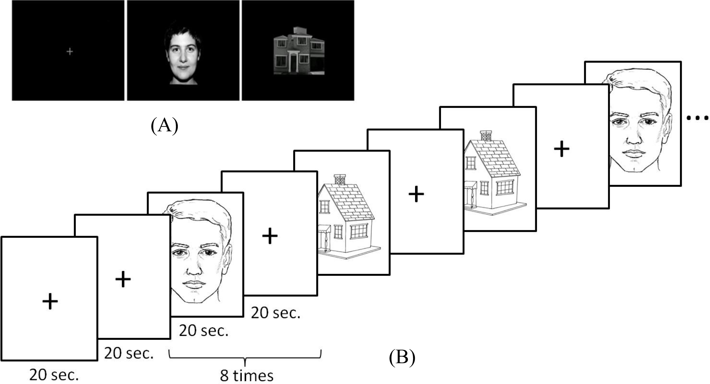$A$ shows typical images of the presented visual stimuli; left to right: Relaxation period, Faces and Buildings. Panel $B$ shows the experimental paradigm of each scan sequence, consisting of 18 blocks of 20 seconds each.

Figure 2.

Stimulation paradigms employed in each of the four sequences of scans. By placing the four paradigms one after the other a sequence of 1440seconds is obtained in which 720 volumes were acquired.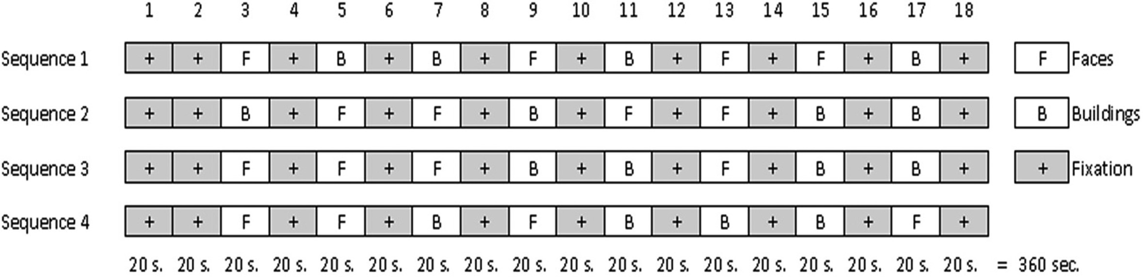

2.3 Acquisition of the fMRI data

fMRI data were acquired at the Instituto Nacional de Psiquiatría Ramón de la Fuente located in Calzada México Xochimilco No. 101 Tlalpan, México.

Subjects were scanned with a MR scan of 3 Tesla (Philips Achieva) using the BOLD contrast with echo planar images (TR $=$ 2 s, TE $=$ 40 ms, 58 $\times$ 40 voxels, voxel size 4 $\times$ 4 $\times$ 4 mm.). To cover the whole brain 46 slices were acquired.

For visual presentation of stimuli, high resolution audiovisual equipment Avotec was used, employing the Silent Vision projector model, which is compatible with the MR scanner used. This equipment was controlled by a Mac running the Psychophysics toolbox version 2.44 under MATLAB. For synchronization between the stimulus presentation and the acquisition of MR images, a response system for RM (Cedrus brand, Lumina model) was used.

2.4 Pre-processing

Data were preprocessed using BrainVoyager QX 2.0 and MATLAB. All volumes were realigned and both spatial and intensity normalizations were applied.

2.4.1 Realigning

Due to involuntary movements of the subject’s head within the magnet, a realignment is necessary. The realigning consists of estimating the difference in position between the different volumes of the same subject. To correct the images’ positions, transpositions and proper rotations compensating this difference are applied [32].

2.4.2 Spatial normalization

Due to the the differences in size and shape among brains it is necessary to transform the original fMRI images to a normalized coordinates system in order to map the voxels of one brain to those in another. To achieve this, an elastic deformation of fMRI images is performed in order to adjust them into the coordinate system of a standard brain known as the Talairach-Tournoux coordinate system [11].

After this transformation, each brain should have the same shape and size, though the transformation is usually imperfect.

2.4.3 Intensity normalization

The intensity of the hemodynamic response to a particular stimulus varies among individuals, so it is recommended [21] to normalize the intensities by re-scaling the data from different subjects in order to match them in the same range (minimum-maximum).

The intensity normalization process was performed in MATLAB using Eq. (1) [31].

$Y_{t}=\frac{X_{t}-\min_{t}X_{t}}{\max_{t}X_{t}-\min_{t}X_{t}}$ (1)

Where $X_{t}$ and $Y_{t}$ represent the data before and after normalization, respectively, while $\min_{t}X_{t}$ represents the minimum value of activations within the volume $t$ and $\max_{t}X_{t}$ represents the maximum value. This method linearly re-scales each voxel’s data to a range of $[0-1]$ .

2.5 Feature selection

After the pre-processing stage, the voxels that serve as features in the classification process were selected. This step is very important for the classification process, because of the great number of voxels in a volume (more than $10^{5}$ ), it is necessary to select only those that allow for better discrimination between classes.

The commonly used methods for feature selection are:

•
Discrim, which consists of selecting the N most discriminative voxels by a pre-classification stage where each voxel is scored by its discriminative capacity [21, 27].
•
Searchlight-Accuracy method, which is similar to Discrim method but instead of using the data from a single voxel use the data from the voxel and its immediately adjacent neighbors in three dimensions [27].
•
Active, which consists on select by regression the N most active voxels based on their ability to distinguish between classes or stimuli, in this case, a statistical test is applied to order the voxels according to the level of activity that had each voxel when each of stimulus was presented [21, 27].
•
roiActive; where an expert defines Regions of Interest (ROI) and the most active voxels inside each ROI are selected [21, 27].

The roiActive technique has the disadvantage that it requires the intervention of an expert who defines the Regions of Interest, and methods that use a pre-classification stage as Searchlight and Discrim, according to Pereira et al. [27] can be computationally expensive.

In a study conducted by Mitchell et al. [21] the above methods were compared and the Active method reached one of the best results, nevertheless the parameter N can make the difference in the classification stage because its value is not very intuitive, have been reported values from 4-2000; this inconvenience has been overcome choosing only the voxels whose $p$ -value (in the statically test) is below to certain threshold, this approach have been broadly used [6, 19].

In our proposal the feature selection stage was integrated by two sections; in the first one, the Active method was applied in order to identify the most active voxels by subject, subsequently, the identified voxels were filtered by a Gaussian Kernel (GK), wich allowed identifying the most discriminative voxels inter-subject. Our contribution is included in this second section where the feature selection among subjects is made.
2.5.1 Section one; feature selection by Active method

The general linear model is described as:

$Y=X\beta+\epsilon$ (2)

Where $\beta$ is the projection parameter and the amount $\epsilon$ represents the error caused by the additive noise.

The variable $Y$ represents a time series of length $n$ (in this case $n=$ 720) for each voxel (Fig. 3A), which can be approximated by a linear combination of the time series in $X$ .

The $X$ matrix of dimensions $(n,p)$ contains the $p$ effects that may have an influence on the acquired signal corresponding to these stimulation patterns, represented as $n$ element vectors (Fig. 3C). Initially these vectors are generated with values of ones and zeros, the ones representing the times in which a stimulus was visually presented (faces or buildings) and the zeros representing periods of relaxation (fixation); These vectors were then convolved [13] with a canonical hemodynamic response function (Fig. 3B).

Once the regression of the data on the stimulation patterns was made, the contrast operation among stimuli [28, 12] was performed, in order to detect those voxels whose activity was statistically significant.

Figure 3.

Stimulation patterns. (A) Voxel’s time series. (B) Time course of the canonical hemodynamic response function: after a stimulation pulse or event, increased BOLD signal starts 2 or 3 seconds later and reaches its peak about 5 seconds later, followed by a decline lasting up to 30 seconds [26]. (C) Stimulation patterns, faces, and buildings, convolved.

The voxels that obtained a $p$ -value $<$ 0.05 (corrected) were then selected. This set of voxels was those which showed a statistically significant response to each stimulation paradigms (faces or buildings), which allows us to know the activation areas by subject related to visual stimuli presented. Figure 4A shows the brain volume of one of the eighth subjects, the volume is composed for 40 axial slices, blue points represent the positions for the voxels selected as features for the faces class and red points represent the positions of the voxels selected for the buildings class.

From these selected voxels a volume of activations per subject was generated (Fig. 4B), represented by a three dimensional matrix (58 $\times$ 40 $\times$ 46) positions, wherein each position represents a voxel and may contain values of 0,1 or 2. A 1 indicates that the voxel was significant (or selected as feature) for faces, a 2 for buildings and a 0 for neither.

Figure 4.

Voxels most significant for each stimulation paradigm (faces or buildings) identified in a subject. (A) Most significant voxels per axial slice. (B) Volume of activations of a subject.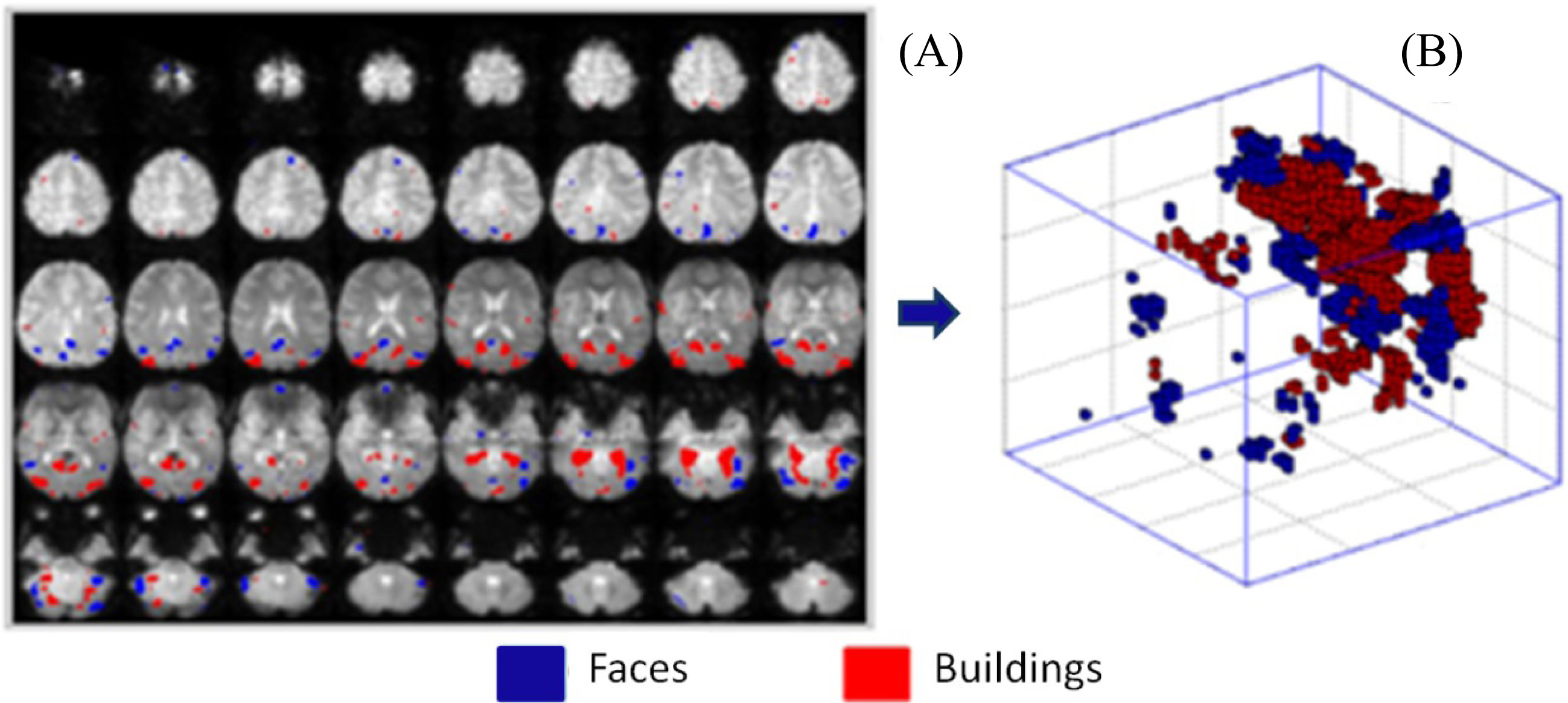

2.5.2 Section two; feature selection by Gaussian kernel

The first step in this section is the generation of a Common Volume of Activation (CVA) where all activations for each of the subjects in the training set were integrated, the CVA is a matrix of (58 $\times$ 40 $\times$ 46) positions with values $[0,1,2]$ .

Figure 5.

Common volume activation. To the left, the volumes of the training set are shown, right the common volume of activations spawned from the training set.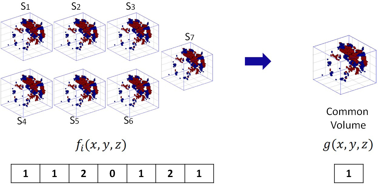

The definition of the value for each CVA position $(x,y,z)$ was made based on the most repeated value in the volumes of the training set with that same position, Eq. (3) summarizes this operation.

$g(x,y,z)=mode[f_{1}(x,y,z),f_{2}(x,y,z),\ldots,f_{N}(x,y,z)]$ (3)

Where $f_{i}(x,y,z)$ represents the value found at position $(x,y,z)$ of the subjects’ activations volume for subject $i$ , for $i=[1,2,\ldots,N]$ , where $N$ represents the number of subjects in the training dataset (Fig. 5). As mentioned in the first part of this article, even with the spatial normalization, functionally equivalent activations between subjects are not necessarily presented in the same position; due to this, it was considered necessary to find a method of inter subjects feature selection that would allow some degree of spatial freedom to find activations in a periphery or neighborhood. Hence this proposal is inspired by the classification algorithm k-nearest neighbor (K-NN). The concept of K-NN, introduced by Fix and Hodges [10], is based on the assumption that the similar instances are probably close in feature space. K-NN is based on a set of instances previously classified; upon wishing to classify a new instance $x$ , the $k$ closest examples to it (in terms of distance) are obtained, for example the Euclidean distance [15], this allows us to assign $x$ the class to which the majority of its $k$ nearest neighbors belong to (Fig. 6A). There are a number of variants of the K-NN algorithm; one of them was proposed by Dudani [7], who questions the fact that each of the $k$ neighbors has the same weight in the classification when not all are at the same distance from the example to classify. Dudani proposes a weighted K-NN where the nearest neighbors have more influence in the classification of $x$ .

Figure 6.

(A) K-nearest neighbors: in this example, for 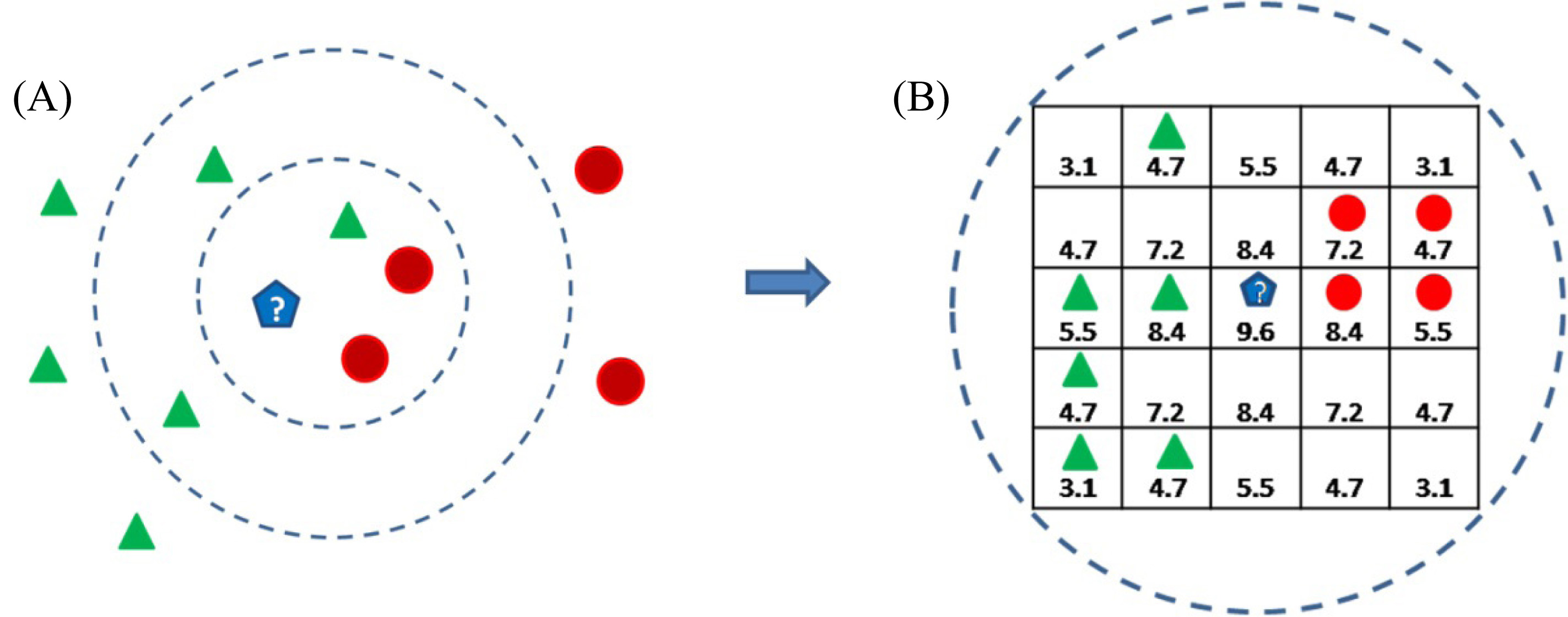$k=$ 3 the new instance is assigned to the class circles, for $k=$ 5 it is assigned to the triangles class. (B) Voxels’ selection using a variation of the k-NN algorithm weighted by a Gaussian distribution: in the example just shown the kernel in 2 dimensions, the new voxel will be selected as an important feature for the stimuli faces (triangles) or buildings (circles) even could not be selected, according with the highest weighting in the isotropic space.

The second step for this section is based on the central idea of Dudani’s algorithm. To contend against the anatomical and functional variability among subjects, we propose defining the activity of a voxel as a weighted vote on the activity observed in its neighbors located on a periphery, which in this case is defined by an isotropic three-dimensional space, as opposed to K-NN where neighbors are located in the feature space. Neighbors defined in this space are taken from the brain activity of subjects in the training set, namely of the CVA, and its influence for selecting a voxel is determined by a Gaussian radial function so that the nearest neighbors are weighted more heavily (Fig. 6B).

The isotropic space in question is defined by a Gaussian kernel. Kernel concept is commonly used in the analysis of digital images [14] to refer to a filter, matrix or $N\times N$ window. In our case the concept is taken into three dimensions, whereby the kernel is represented by a three-dimensional matrix, or a Gaussian cube with dimensions of $N\times N\times N$ , where $N$ is an odd number. For example, for $N=5$ a three-dimensional matrix (5 $\times$ 5 $\times$ 5) is generated and the values for each of their positions (weights) are calculated based on the Gaussian distribution defined by Eq. (4), centered on the position $(x,y,z)$ of the voxel to be selected and a standard deviation $\sigma$ .

$G_{3D}(x,y,z;\sigma)=\frac{1}{(\sqrt{2\pi\sigma})^{3}}e^{\frac{x^{2}+y^{2}+z^{% 2}}{2\sigma^{3}}}$ (4)

This Gaussian kernel represents the isotropic space, in which the neighbors that will allow us to classify a new instance will be searched; the assigned weights represent the influence that each neighbor will have in the voxel selection process.

Formally, let $l=\{1,2\}$ the set of labels in a common $f$ activation volume with dimensions $(X\times Y\times Z)$ . In our case, label $1$ represents the label faces while the label $2$ represents buildings. The CVA $f$ is generated with the data of the subjects in the training set as was explained above.

Let $q$ be the activations volume of the test subject, whose dimensions are the same as for $f$ and whose initial values were set to be equal to $0$ . To select a voxel as an important feature for each stimuli, its label at position $(x,y,z)$ with a Gaussian cube $w$ of $N\times N\times N$ will be calculated as:

$q(x,y,z)=\textit{label}_{\max}(g(x,y,z,l_{i}))$ (5)

Thus the label for $q$ in the $(x,y,z)$ position will be that which is associated with the maximum value in $g(x,y,z,l_{i})$ for $i=[1,2]$ .

As in our case we only have two labels, the above expression can be expressed in an expanded form as:

$q(x,y,z)=\textit{label}_{\max}(g(x,y,z,1),g(x,y,z,2))$ (6)

For the function $g(x,y,z,l_{i})$ , this one is defined as:

$g(x,y,z,l_{i})=\sum_{s=-a}^{a}\sum_{t=-a}^{a}\sum_{u=-a}^{a}(w(s,t,u)h(x+s,y+t% ,z+u,l_{i}))$ (7)

Where:

$h(x,y,z,l_{i})=\begin{cases}1&{\rm if}∼{}f(x,y,z)=l_{i}\\ 0&\rm otherwise\end{cases}$ (8)

for $a=(N-1)/2$ .

To mark a voxel as an important feature, the neighbors that might exist in a cube of $N\times N\times N$ are sought, where the new voxel is considered to be located in the center of the cube. $N$ represents the length in voxels of each of the sides of the cube and can take any odd integer number value.

Each of the possible labeled neighbors’ CVA (within this neighborhood bounded by the cube) issues a vote and the new voxel is selected according to the label that receives the most votes, taking into consideration that the neighbors’ vote is different, depending on how close they are to the center of the cube, the voting center’s closest neighbors have greater weight.

2.6 Creating database

As mentioned previously the entry data in a classification task are assigned through a database where each record or example is composed by a set of attributes and one class.

Once finished the previous step, a total of $m+n$ attributes (voxels) were selected, $m$ of them are associated with the faces class and are represented as $V_{fi}$ for $i=[1,2,\ldots,m]$ and $n$ to the buildings class, represented as $V_{bj}$ , for $j=[1,2,\ldots,n]$ , see Table 1.

In order to create the examples, the registered values of each of these voxels in the time that lasted each of the blocks of faces or buildings (see Fig. 2) were averaged, this method has been deeply documented in [27]. Thereby 32 examples (16 for the faces class and 16 for buildings) for each of the eight subjects were generated, then a database with 256 examples was built. see Table 1.

Columns labeled as No and Example ID were added for sake of clarity, the first one is a consecutive number for each example and the second one is an identifier, thus $S_{1}E_{32}$ represents the example 32 created with data from subject 1. The F and B labels on the class column represent the faces and buildings class respectively.

Table 1
Database schema used in the classification stage, this consists of $m+n$ attributes and 256 examples

No	Example ID	$V_{f1}$	$V_{f2}$	…	$V_{fm}$	$V_{b1}$	$V_{b2}$	…	$V_{bn}$	Class
1	$S_{1}E_{1}$			…				…		F
2	$S_{1}E_{2}$			…				…		B
…	…	…	…	…	…	…	…	…	…	…
32	$S_{1}E_{32}$			…				…		F
33	$S_{2}E_{1}$			…				…		F
34	$S_{2}E_{2}$			…				…		B
…	…	…	…	…	…	…	…	…	…	…
64	$S_{2}E_{32}$			…				…		F
…	…	…	…	…	…	…	…	…	…	…
225	$S_{8}E_{1}$			…				…		F
226	$S_{8}E_{2}$			…				…		B
…	…	…	…	…	…	…	…	…	…	…
256	$S_{8}E_{32}$			…				…		F

2.7 Classification and evaluation of the performance of the classifier

Once the database was created as described in the previous step it was necessary to choose the most appropriate classification algorithm for the experiment in question.

The classification of cognitive states has been addressed with several classifiers, both linear and non-linear classifiers [21, 27], however authors such as Mur [22] have found that linear classifiers as minimum-distance classifier, Fisher linear discriminant analysis (FLDA) and the linear support vector machine (SVM) are the most widespread and successful tool for pattern-information analysis in neuroimaging.

This is also accepted by Pereira [27], y Norman [24] due than non-linear classification methods are more prone to overfit the data than linear classification methods and overfitting is a particularly problem in fMRI due to the great difference between the high number of attributes and a small number of examples.

In addition Mitchell [21], Pereira [27] and Mahmoudi [19] argue than SVM is a good choice of lineal classifier for binary classification and with multiple-subject, which adjusts perfectly to the type of experiment in question, for this reason we chose the SVM classifier.

The validation process was performed using the technique of leave-one-out cross-validation. In this technique, the data set of $n$ elements, considering here $n$ as the number of subjects, is divided into n subsets, and the classifier is trained with examples from $n-1$ subjects (training dataset) verifying the accuracy of the classifier with the data of the remaining subject. This process is repeated $n$ times and in each one the classifier’s accuracy is evaluated with a different subject.

For purposes of this experiment the training set was composed by 224 examples of 7 subjects. Feature selection was performed with data from these 7 subjects, the CVA was generated and the SVM classifier was trained, then it was evaluated with the 32 examples from the remaining subject.

In each test the accuracy, sensitivity and specificity of the classifier were calculated. The sensitivity represents the proportion of faces correctly predicted while the specificity represents the proportion of buildings correctly predicted.

Finally, a total of eight accuracies, eight sensitivities and eight specificities were obtained, from which the average and standard deviation of each one were calculated to determine the performance of the algorithm.

The results obtained by the proposed Gaussian Kernel method were compared against Active method and the 95% confidence Wilcoxon test was applied.

3. Results

In order to evaluate the performance of Gaussian Kernel method two experiments were carried out. In the first one, the optimal size of Gaussian Cube was determined, and in the second one the performance of Gaussian Kernel method was compared against the Active method.

3.1 Experiment 1: Size of gaussian cube

Preliminary tests were made employing cubes of different sizes in the feature selection stage; it was observed that with cubes of sizes 3, 5, 7, 9 and 11 the best accuracies were obtained in the classification stage using the SVM algorithm. The results for cubes above 11 are not reported due to the fact that in these cases, a sharp drop in the classifier’s accuracies below 63.28% were observed.

In the case of a 3 $\times$ 3 $\times$ 3 cube the accuracy was of 90.23%; with cube of a size of 5 $\times$ 5 $\times$ 5 an accuracy of 96.48% was obtained, this was the best accuracy; for the 7 $\times$ 7 $\times$ 7 cube, accuracy was 90.63%, while the 9 $\times$ 9 $\times$ 9 cube generated 90.23% accuracy. 11 $\times$ 11 $\times$ 11 cubes’ accuracy was of 89.84%.

In this test, it was also observed that the number of selected activations (namely attributes or characteristics) for buildings class was greater than the ones for faces class: there is in general a 70% of selected activations for buildings and a 30% for faces. This indicates that the number of voxels with significant activity and that are related to buildings class is greater than the number of voxels related faces. The above is not a problem for the classification algorithm, since it receives as input the attributes related to both classes.

3.2 Experiment 2: A comparison against Active method

Having determined that the Gaussian cube sized 5 $\times$ 5 $\times$ 5 allowed us to obtain the best accuracies, these results were compared against those obtained by the Active method, and this comparison is presented in Table 2. In all these tests a $p$ -value $<$ 0.05 (Bonferroni corrected) and a standard deviation $\sigma=1$ was used.

Table 2
Comparison of the sensitivity, specificity and accuracy results obtained in the classification stage by the Active feature selection method, against those obtained by Gaussian Kernel (GK) method when using a 5 $\times$ 5 $\times$ 5 cube, ‘ $+$ ’ means that there was a significant difference favoring the proposed method with respect to the Active method

Subject No.	Sensitivity		Specificity		Accuracy
	Active	GK	Active	GK	Active	GK
1	75.00	87.50	93.75	100.0	84.38	93.75
2	75.00	100.0	87.50	100.0	81.25	100.00
3	87.50	93.75	75.00	93.75	81.25	93.75
4	75.00	100.0	87.50	93.75	81.25	96.88
5	87.50	100.0	81.25	100.0	84.38	100.0
6	87.50	93.75	93.75	100.0	90.63	96.88
7	81.25	93.75	93.75	93.75	87.50	93.75
8	75.00	93.75	93.75	100.0	84.38	96.88
Mean	80.47	95.31 ${}^{+}$	88.28	97.66 ${}^{+}$	84.38	96.48 ${}^{+}$
SD	6.19	4.42	7.04	3.23	3.34	2.61

Figure 7.

Confusion matrix for the Active method (left) and the Gaussian Kernel method (right).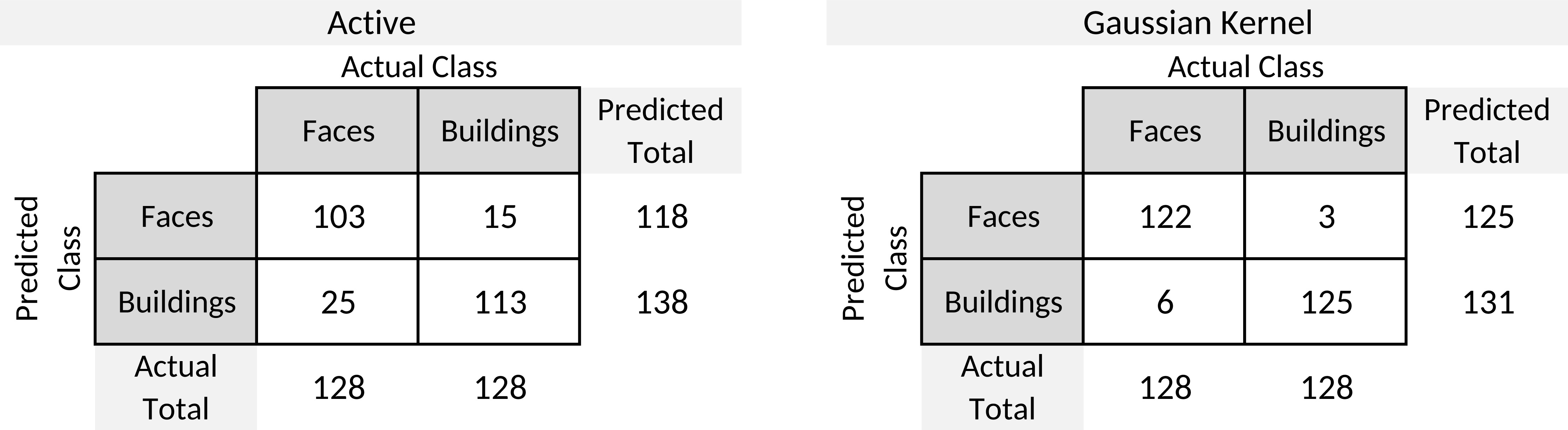

Table 2 shows the sensitivity, specificity and accuracy results obtained by SVM classifier. Note than the sensitivity represents the proportion of faces correctly predicted while the specificity represents the proportion of buildings correctly predicted.

The results obtained by employing a Gaussian cube of (5 $\times$ 5 $\times$ 5) voxels indicates that by using this cube, the activation value of a voxel is affected by activations that are within $\pm$ 2 voxels (8 mm) given that as mentioned above, when a new voxel is selected, it is located in the center of a Gaussian cube of a dimension of $(N\times N\times N)$ voxels, where each voxel equals (4 $\times$ 4 $\times$ 4) mm. It is therefore assumed that the activation of a voxel is influenced by activations found within a $\textit{radius}=(((N-1)*4)/2)$ mm.

As shown in Table 2, with the Active method a minimum sensitivity of 75.00%, a maximum of 87.5% and an average of 80.47% with a standard deviation of 6.19 was obtained, whereas the Gaussian Kernel method obtained a minimum sensitivity of 87.5%, a maximum of 100% and an average of 95.31% with a standard deviation of 4.42.

In the specificity results, the Active approach obtained a minimum of 75.00%, a maximum of 93.75% and an average of 88.28% with a standard deviation of 7.04; whereas the proposed method obtained a minimum of 93.75%, a maximum of 100% and an average of 97.66% with a standard deviation of 3.23.

As pertains to accuracy, the Active approach obtained a minimum of 81.25%, a maximum of 90.63% and an average of 84.38% with a standard deviation of 3.34, while the minimum accuracy obtained with the Gaussian 5 $\times$ 5 $\times$ 5 cube was of 93.75%, with a maximum of 100% and an average accuracy of 96.48% with a standard deviation of 2.61.

As shown in these results, in sensitivity (Wilcoxon, $p=$ 6.216E-4), specificity (Wilcoxon, $p=$ 0.0054) and accuracy (Wilcoxon, $p=$ 1.554E-4) the Gaussian Kernel of 5 $\times$ 5 $\times$ 5 obtained best results than the Active method. In all three cases the findings show a statistically significant difference close to 10 percentage points favoring the proposal approach.

Finally Fig. 7 shows the confusion matrices generated from Active method (left) and the proposed method with a Gaussian cube of 5 $\times$ 5 $\times$ 5 (right). These matrices capture the total of 256 examples classified, 128 per class (32 examples per subject), and as can be seen, the proposed method makes fewer errors to assign the database examples both classes than the traditional method.

4. Discussion

For the second experiment, the same SVM classifier was trained, with the same data, only changing the feature selection method; both methods pick out the features from the data in the training set, with the difference that Active method considers the same spatial positions among subjects, whereas in the Gaussian Kernel method the positions in a radius of 8 mm. are considered. Since to with the Active method the lowest accuracies were obtained, this allows us to suppose that there is variability in the spatial location of the activations for the same stimulus among subjects.

When cubes above 11 voxels were used very low accuracies were obtained because the isotropic space is very broad, which reflect the influence of activations located on a radius greater than or equal to 24 mm, and therefore, the selected voxels are influenced by activations of very different functional areas.

On the other hand, when cubes of size 3, 5, 7, 9 and 11 were used, accuracies above 89.8% were obtained, which may be because the classification was made based on the activations that occurred in a radius of 4, 8, 12, 16 and 20 mm.

The best results were obtained when using a 5 $\times$ 5 $\times$ 5 voxels cube, considering that each voxel dimension was 4 $\times$ 4 $\times$ 4 mm, and cube size was 20 $\times$ 20 $\times$ 20 mm. In this case the variation from one individual to another was produced within an approximate radius of 8 mm ( $\pm$ 2 voxels), without considering the central voxel as when a new voxel is selected it is considered to be found in the center of the cube, this is why neighboring activations seek each other within a radius of 8 mm.

This is an important finding consistent with the fact that when adjusting the brains of different subjects to a common space an error of about ten millimeters [21, 3] is generated, as well as the fact that that there is variation in the location of functional areas among subjects ranging from 3 to 15 mm on average [33, 16, 1] and the fact that the activity patterns associated with the same cognitive status are often different among subjects [17].

In previous section, was mentioned the fact of the differences in the quantity of activations selected by class. It was observed a largest quantity of activations related with buildings class; according to the reported in [29] it is explained because the cortical areas involved in the perception of buildings is larger than the involved in the perception of faces.

The accuracy obtained with the Active feature selection method, were lower than those obtained with the Gaussian Kernel method since the latter allows the classification of a new instance based on voxels selected with a tolerance limited by an isotropic three-dimensional space which contains only the most repeated activations in the training set, furthermore the vote of each activation does not have the same weight, the activations closest to the center have a higher weight modeled by a Gaussian function, this is what allows to decrease the margin of error in the classification process.

With reference to the database size, although it has a small number of individuals, statistically can be inferred that by increasing the number of subjects there will still be a statistically significant difference favoring the proposed method, additionally, by increasing the training data set, the classifier will be more robust, preserving or improving the accuracy reported; in words of Tom Mitchell [21] “…the accuracy of SVM’s increases relatively as the number of training examples increases…”.

On the other hand, with a larger training data set, in the stage where the generation of CVA is performed, more voters will be obtained, which would allow a better selection of inter-subject features.

In this kind of studies, whose purpose is the inter-subject classification of cognitive states, tests are performed in healthy subjects, just as this study was conducted, therefore, considering the results obtained, we can assume that the proposed technique is reliable for this group of subjects; however, in practice the inter-subject classification also has been used with unhealthy people to the prediction of diseases [20].

For unhealthy people, the inter-subject classification has been used as a biomarker, for example in predicting Alzheimer’s disease (AD) [35] or for identify major depressive individuals from healthy controls [34], where usually, there are two class labels: healthy individuals and patients, and the experimental designs are performed according to the type of disease to be predicted.

Under this scheme, the type of feature selection proposed here could distinguish more efficiently between one group or another because neural activations, or lack thereof, is often different between these groups of people and this same will create a more reliable CVA since this is performed by voting.

The Intelligence Quotient (IQ) of the study group was not measured, in previous studies of this kind also has not been reported if the IQ can make a significant difference in the accuracy of the classification model, this seems to be an open question that can be addressed in future studies.

5. Conclusions and future work

fMRI data analysis has evolved significantly in recent years, and is now seen as an important tool in the field of neuroscience. Group analysis points to the generation of new techniques that result in a better understanding of brain function. These techniques could also be used as possible tools for the diagnosis of mental disorders such as schizophrenia or depression [34].

In this context, this work provides an enhancement to the group classification of cognitive states in fMRI by proposing an approach that seeks to contend with the anatomical and functional variability among subjects where there is no need for expert intervention to define regions of interest. The proposed method allows the voxels selection for the classification of new instances based on the weighted voting of its nearest voxels located in an isotropic three-dimensional space, thereby enabling the comparison of neural activity among subjects in similar spatial positions with a tolerance threshold.

The results obtained encourage us to propose the use of this algorithm in the features selection stage when a group classification of cognitive states based on functional Magnetic Resonance Images is made, as it allows for the data analysis among subjects with a higher level of accuracy without the need for predefined regions of interest. Additionally, the proposed method can be used also for data analysis from other techniques to record neural activity as Positron Emission Tomography (PET).

One suggestion for future work is to combine our method with other methods commonly used for group analysis [21]. This method could be used to avoid defining regions of interest. It could be implemented after the generation of a common volume in order to find the connected components, and then process them as a single region of interest.

Finally, another possibility for future studies consists of comparing the performance of this method with the algorithms commonly used in the group classification of cognitive states where regions of interest are typically defined.

Footnotes

Acknowledgments

This research was supported in part by PAPIIT-DGPA IN221413-3 grant. English grammar and style correction were performed by Santiago Fernandez.

References

Allen

E.A.

Erhardt

E.B.

Wei

Eichele

and Calhoun

V.D.

, Capturing inter-subject variability with group independent component analysis of fmri data: A simulation study, Neuroimage 59(4) (2012), 4141–4159.

Allison

Ginter

McCarthy

Nobre

A.C.

Puce

Luby

and Spencer

D.D.

, Face recognition in human extrastriate cortex, Journal of Neurophysiology 71(2) (1994), 821–825.

Ashburner

and Friston

, Multimodal image coregistration and partitioning – a unified framework, Neuroimage 6(3) (1997), 209–217.

Berman

M.G.

Park

Gonzalez

Polk

T.A.

Gehrke

Knaffla

and Jonides

, Evaluating functional localizers: The case of the ffa, NeuroImage 50(1) (2010), 56–71.

Carlson

T.A.

Schrater

and He

, Patterns of activity in the categorical representations of objects, Journal of Cognitive Neuroscience 15(5) (2003), 704–717.

de Beeck

H.P.O.

Brants

Baeck

and Wagemans

, Distributed subordinate specificity for bodies, faces, and buildings in human ventral visual cortex, Neuroimage 49(4) (2010), 3414–3425.

Dudani

S.A.

, The distance-weighted k-nearest-neighbor rule, Systems, Man and Cybernetics, IEEE Transactions on (4) (1976), 325–327.

Epstein

and Kanwisher

, A cortical representation of the local visual environment, Nature 392(6676) (1998), 598–601.

Experimentation

, Human experimentation: Code of ethics of the world medical association (declaration of helsinki), Canadian Medical Association Journal 91(11) (1964), 619–619.

10.

Fix

and Hodges

J.L.

, Jr., Discriminatory analysis-nonparametric discrimination: Consistency properties, Technical report, DTIC Document, 1951.

11.

Friston

Ashburner

Frith

C.D.

Poline

J.-B.

Heather

J.D.

Frackowiak

R.S.

et al., Spatial registration and normalization of images, Human Brain Mapping 3(3) (1995), 165–189.

12.

Friston

K.J.

Holmes

A.P.

Worsley

K.J.

Poline

J.-P.

Frith

C.D.

and Frackowiak

R.S.

, Statistical parametric maps in functional imaging: A general linear approach, Human Brain Mapping 2(4) (1994), 189–210.

13.

Friston

K.J.

Worsley

K.J.

Frackowiak

Mazziotta

J.C.

and Evans

A.C.

, Assessing the significance of focal activations using their spatial extent, Human Brain Mapping 1(3) (1994), 210–220.

14.

Gonzales

R.C.

and Woods

R.E.

, Digital image processing, New Jersey: Prentice Hall 6 (2002), 681.

15.

Han

Kamber

and Pei

, Data Mining: Concepts and Techniques, Elsevier, 2011.

16.

Hasnain

M.K.

Fox

P.T.

and Woldorff

M.G.

, Intersubject variability of functional areas in the human visual cortex, Human Brain Mapping 6(4) (1998), 301–315.

17.

Heaven

, Mind-reading the meaning of words, New Scientist 216(2891) (2012), 8.

18.

Kanwisher

McDermott

and Chun

M.M.

, The fusiform face area: A module in human extrastriate cortex specialized for face perception, The Journal of Neuroscience 17(11) (1997), 4302–4311.

19.

Mahmoudi

Takerkart

Regragui

Boussaoud

and Brovelli

, Multivoxel pattern analysis for fmri data: A review, Computational and Mathematical Methods in Medicine 2012 (2012).

20.

Martínez-Ramón

Koltchinskii

Heileman

G.L.

and Posse

, fmri pattern classification using neuroanatomically constrained boosting, Neuroimage 31(3) (2006), 1129–1141.

21.

Mitchell

T.M.

Hutchinson

Niculescu

R.S.

Pereira

Wang

Just

and Newman

, Learning to decode cognitive states from brain images, Machine Learning 57(1–2) (2004), 145–175.

22.

Mur

Bandettini

P.A.

and Kriegeskorte

, Revealing representational content with pattern-information fmri – an introductory guide, Social Cognitive and Affective Neuroscience (2009), nsn044.

23.

Nieto-Castanon

Ghosh

S.S.

Tourville

J.A.

and Guenther

F.H.

, Region of interest based analysis of functional imaging data, Neuroimage 19(4) (2003), 1303–1316.

24.

Norman

K.A.

Polyn

S.M.

Detre

G.J.

and Haxby

J.V.

, Beyond mind-reading: multi-voxel pattern analysis of fmri data, Trends in Cognitive Sciences 10(9) (2006), 424–430.

25.

Peelen

M.V.

Fei-Fei

and Kastner

, Neural mechanisms of rapid natural scene categorization in human visual cortex, Nature 460(7251) (2009), 94–97.

26.

Penny

W.D.

Friston

K.J.

Ashburner

J.T.

Kiebel

S.J.

and Nichols

T.E.

, Statistical Parametric Mapping: The Analysis of Functional Brain Images: The Analysis of Functional Brain Images, Academic press, 2011.

27.

Pereira

Mitchell

and Botvinick

, Machine learning classifiers and fmri: A tutorial overview, Neuroimage 45(1) (2009), S199–S209.

28.

Poline

Kherif

Pallier

and Penny

, Contrasts and classical inference, Stat Parametr Mapp Anal Funct Brain Images Anal Funct Brain Images (2011).

29.

Sung

Y.-W.

and Ogawa

, A property of face representation at the categorical level, Neuroscience Letters 448(1) (2008), 1–5.

30.

Tan

P.-N.

Steinbach

Kumar

et al., Introduction to Data Mining, volume 1, Pearson Addison Wesley Boston, 2006.

31.

Wang

Mitchell

T.M.

and Hutchinson

, Using machine learning to detect cognitive states across multiple subjects, CALD KDD Project Paper (2003).

32.

Woods

R.P.

Cherry

S.R.

and Mazziotta

J.C.

, Rapid automated algorithm for aligning and reslicing pet images, Journal of Computer Assisted Tomography 16(4) (1992), 620–633.

33.

Xiong

Rao

Jerabek

Zamarripa

Woldorff

Lancaster

and Fox

P.T.

, Intersubject variability in cortical activations during a complex language task, Neuroimage 12(3) (2000), 326–339.

34.

Zeng

L.-L.

Shen

Liu

Wang

Fang

Zhou

and Hu

, Identifying major depression using whole-brain functional connectivity: a multivariate pattern analysis, Brain 135(5) (2012), 1498–1507.

35.

Zhang

Wang

Zhou

Yuan

Shen

Initiative

A.D.N.

et al., Multimodal classification of alzheimer’s disease and mild cognitive impairment, Neuroimage 55(3) (2011), 856–867.

A feature selection method based on a neighborhood approach for contending with functional and anatomical variability in fMRI group analysis of cognitive states

Abstract

Keywords

1. Introduction

2. Materials and methods

2.1 Participants

2.2 Experimental design

2.4 Pre-processing

2.4.1 Realigning

2.4.2 Spatial normalization

2.4.3 Intensity normalization

Table 1 Database schema used in the classification stage, this consists of m + n attributes and 256 examples

3. Results

3.1 Experiment 1: Size of gaussian cube

3.2 Experiment 2: A comparison against Active method

5. Conclusions and future work

Footnotes

Acknowledgments

References

Table 1
Database schema used in the classification stage, this consists of $m+n$ attributes and 256 examples