A probabilistic model selection criterion for spectral clustering

Abstract

Model selection in spectral clustering consists in estimating the ground truth number of clusters $K^{*}$ . We propose a novel probabilistic framework to address this problem in a principled manner. The spectral clustering pipeline relies on a latent representation over which a mixture model with $K$ components is eventually fitted. However the dimensionality of the latent representation varies alongside $K$ : this setting is uncommon in the literature on mixture model selection. This raises issues regarding probabilistic modelling, and leads to the ineffectiveness of classical criteria such as the Bayesian Information Criterion (BIC). Alternatively, we propose an adapted Gaussian likelihood expression, and use it to derive a probabilistic model selection criterion for spectral clustering. We give theoretical arguments and empirical evidence suggesting the proposed criterion mitigates the peculiarities observed with classical criteria in an effective way. The performance of the method is evaluated on real and synthetic data sets, and compared to concurrent approaches from the literature.

Keywords

Spectral clustering model selection

1. Introduction

Clustering is pervasive in data-intensive practices. Basically, this class of techniques automatically extracts homogeneous groups from unlabeled data, which is often useful in exploratory stages of an analysis, or for preprocessing data before a supervised learning task. Relevant applications include the identification of health care trends from medical records [26], the processing of hyperspectral images to identify novel objects in the sky [30], speaker identification and speech processing [16].

A limitation of the most common clustering techniques such as k-means is the inability to extract non-convex clusters, i.e., those that lie on non-linear low-dimensional manifolds within a higher dimensional space. Spectral clustering proceeds by unfolding such clusters to a transformed space where they can more easily be extracted. Most spectral clustering variants assume the number of clusters is known in advance, which is seldom the case in exploratory data analysis.

This model selection problem has been addressed in various ways in the literature. In the range of non-parametric models adapted to non-convex clusters, Self-Organizing Maps let the user choose the number of clusters using visual cues, as facilitated by the low-dimensional mapping of the data they produce [23]. It is chosen automatically in DBSCAN, solely influenced by a threshold parameter [17]. This parameter is set heuristically using the distribution of pairwise distances among elements of the data set. Similarly, Mean Shift determines the number of clusters automatically, but it is ultimately linked to a bandwidth parameter, also set heuristically [14]. In the affinity propagation technique proposed by [20], the clusters emerge iteratively from exemplars. To the contrary of previously mentioned techniques, its damping factor parameter is data-independent.

Elaborate procedures for model selection exist in the context of parametric mixture models. Beyond the traditional Bayesian Information Criterion (BIC) [31], more recently variational methods [3] and Dirichlet mixture models [28] have been proposed. Heuristics specially crafted to spectral clustering have also been proposed in the literature [42, 39]. Yet the ultimate step of the spectral clustering processing pipeline relies on a mixture model formalism, and to our knowledge little has been made to leverage parametric mixture selection methods such as [31] or [3] in this context.

1.1 Our contributions

As the model selection problem is quite general, and often addressed in model-specific ways, we focus our review of related work to model selection for spectral clustering in Section 2. We show traditional mixture model selection criteria such as BIC are not adapted to the structure underlying the spectral clustering problem in Section 3. In response, we propose a Dimensionality-Independent Gaussian likelihood expression as an adapted probabilistic scheme. We conduct a detailed theoretical and empirical analysis of the properties of this expression. A novel Dimensionality-Independent criterion for spectral clustering model selection is built upon this expression. Section 4 compares its performance to related methods from the literature.

2. Related work

2.1 The spectral clustering algorithm

Let us consider a $d$ -dimensional numerical data set of $N$ elements $\{\mathbf{x}_{1},\dots,\mathbf{x}_{n},\dots,\allowbreak\mathbf{x}_{N}\}$ , with $\mathbf{x}_{n}=\{x_{n1},\ldots x_{nd}\}$ . $d$ is the dimensionality of the data in its initial space. Alternatively the $N$ data elements can be seen as the vertices of a graph, with edges weighted by the similarities between pairs of elements. The graph is implemented by the matrix $\mathbf{S}$ , with $\mathbf{S}_{nn^{\prime}}\in[0,1]$ the similarity between $\mathbf{x}_{n}$ and $\mathbf{x}_{n^{\prime}}$ . Several methods can convert $d$ -dimensional data to a graph: for example, [38] builds a k-NN graph by setting $\mathbf{S}_{nn^{\prime}}=1$ iif elements $n$ et $n^{\prime}$ both belong to their $k$ respective nearest neighbors, 0 else. In this paper, we use the Radial Basis Function (RBF) [27], most commonly used when there is little prior knowledge about the data:

$\displaystyle\mathbf{S}_{nn^{\prime}}=\exp{\biggl{(}-\frac{||\mathbf{x}_{n}-% \mathbf{x}_{n^{\prime}}||^{2}}{\sigma^{2}}\biggr{)}},$ (1)

yielding similarities ranging in $]0,1]$ . Let $\mathbf{D}$ be the diagonal matrix such that $\mathbf{D}_{nn}=\sum_{n^{\prime}=1}^{N}{\mathbf{S}_{nn^{\prime}}}$ , i.e., featuring the node degrees on its diagonal. In the literature, $\mathbf{L}=\mathbf{D}-\mathbf{S}$ is called the Laplacian of graph $\mathbf{S}$ . Normalized variants have been proposed in the literature, among which the most widely used is the symmetric Laplacian $\mathbf{L}_{\text{sym}}=\mathbf{D}^{-\frac{1}{2}}\mathbf{L}\mathbf{D}^{-\frac{% 1}{2}}=\mathbf{I}-\mathbf{D}^{-\frac{1}{2}}\mathbf{S}\mathbf{D}^{-\frac{1}{2}}$ [18, 42].

Spectral clustering proceeds with the eigenvalue decomposition of the Laplacian, written as $\mathbf{U}\Lambda\mathbf{U}^{T}$ . The columns of matrix $\mathbf{U}$ and the diagonal of $\Lambda$ are the eigenvectors and eigenvalues of the Laplacian, respectively. An explicit relationship between the $K$ last columns of $\mathbf{U}$ and the optimum of the relaxed minimal graph cut of matrix $\mathbf{S}$ in $K$ connected components has been established [33, 38], and is summarized by Proposition 1:

.

Let us assume $\mathbf{S}$ exhibits $K$ clusters as the result of a relaxed minimal graph cut. Then:

•

the $K$ last columns of $\mathbf{U}$ are associated to the eigenvalue 0,

•

the range of the $K$ last eigenvectors of L and $\textbf{L}_{\text{sym}}$ has vectors $\mathbbm{1}_{k},k\in\{1\ldots K\}$ as basis,

with $\mathbbm{1}_{k}$ the indicator vector of cluster $k$ . In practice, Proposition 1 implies that membership of data element $\mathbf{x}_{n}$ to one of the clusters can be deduced by inspecting the $n^{\text{th}}$ row of the $K$ last columns of matrix $\mathbf{U}$ . As the range of these columns is the set of $K$ indicator vectors, each row is assigned with 1 out of $K$ distinct $K$ -dimensional vectors, each characterizing a cluster.

The RBF, on which the computation of $\mathbf{U}$ ultimately relies, has one free parameter: $\sigma$ in Expression (1). In the empirical density estimation literature it is often known as the bandwidth [32], as it controls the width of an unnormalized Gaussian. This parameter is often set to a constant without further discussion [20, 25, 40]. [42] proposed a local bandwidth parametrization, which uses a distinct bandwidth parameter for each data element:

$\displaystyle\mathbf{S}_{nn^{\prime}}=\exp{\biggl{(}-\frac{||\mathbf{x}_{n}-% \mathbf{x}_{n^{\prime}}||^{2}}{\sigma_{n}\sigma_{n^{\prime}}}\biggr{)}},$ (2)

[42, 22] empirically set $\sigma_{n}$ with the Euclidean distance of element $n$ to its $7^{\text{th}}$ and $4^{\text{th}}$ nearest neighbor, respectively. In a recent study, additional observations support this parametrization, and a generalization depending on the quantiles of the empirical pairwise distance distribution is proposed [10]. There it is shown that the 2% quantile yields the best results, independently of the data set at hand. In the remainder of the paper, the RBF as stated in Eq. (2) is used, along with the 2% quantile.

Most spectral clustering implementations directly decompose $\mathbf{D}^{-\frac{1}{2}}\mathbf{S}\mathbf{D}^{-\frac{1}{2}}$ instead of the actual symmetric Laplacian. The solution is then associated to eigenvalue 1, which is itself associated to the $K$ major eigenvectors of $\mathbf{D}^{-\frac{1}{2}}\mathbf{S}\mathbf{D}^{-\frac{1}{2}}$ - identical to those of $\mathbf{L}_{\text{sym}}$ up to the sign and the reversed order [18]. More options for efficient partial decomposition are available for the major order (e.g., Lanczos methods [4]): in the remainder of the paper, decompositions are thus implicitly made with reference to this variant. For convenience, we also refer to the $K$ first columns of $\mathbf{U}$ as $\mathbf{U}_{K}$ .

We refer to the $n^{\text{th}}$ coordinates (i.e., line) of $\mathbf{U}_{K}$ as the latent coordinates of element $n$ . The $K$ -dimensional space in which these coordinate vectors take values is then called latent space of the Laplacian. This denomination is to contrast with the initial space in which data is represented, i.e., to which the RBF is applied.

The motivation for spectral clustering is to formalize clusters in terms of neighborhood in a graph, materialized by the transformation of the initial space to a simplified latent space following Proposition 1. As the columns in $\mathbf{U}_{K}$ are rank- $K$ linear combinations of indicator vectors (see Proposition 1), latent coordinate vectors take 1 out of $K$ distinct canonical positions in the latent space, therefore greatly facilitating their processing by the k-means algorithm. The dimensionality of the initial space $d$ then becomes implicit to the similarities, and the complexity of k-means is shifted from $O(d)$ to $O(K)$ , usually small in clustering applications.

2.2 Model selection in spectral clustering

As implied by Proposition 1, there is a link between the number of clusters and the multiplicity of eigenvalue 0 (or 1 if major order is used) in the respective Laplacian. Assuming the ground truth number of clusters is $K^{*}$ , the $K^{*}+1^{\text{th}}$ eigenvalue is then significantly smaller than one, i.e. the eigengap $\lambda_{K^{*}}-\lambda_{K^{*}+1}$ is large. Monitoring this gap is the most classical procedure to determine $\hat{K}$ , the estimate of $K^{*}$ .

The $K^{*}$ first eigenvalues seldom strictly equal 1 in realistic settings, so an approximation is necessary. A simple heuristic has been to find an inflexion point in the curve of eigenvalues ordered in decreasing order [12]. Recently a variant of Bartlett’s test for equal variances has also used this curve of eigenvalues [11].

As the distribution in the latent space is theoretically concentrated on a set of $K^{*}$ canonical positions, [42] perform model selection by estimating the divergence from such a configuration.

[13] use the Approximation Set Coding framework to estimate the $\hat{K}$ that strikes a trade-off between stability and informativeness. They rely on the kernel trick in order to avoid the varying dimensionality of the latent space identified in Sections 2.1. [34] assume an upper bound to $K^{*}$ , and use a dimensionality reduction approach. The link between $K^{*}$ and the latent subspace dimensionality is not used explicitly then.

Some spectral clustering approaches completely avoid the use of Laplacians and eigendecompositions, and use inflation and contraction operators to directly estimate maximal subgraphs [37, 25]. This procedure claims to automatically estimate the number of clusters as a by-product. It has a single parameter that influences the granularity of solutions, i.e., to weight emphasis on small compact clusters.

Figure 1.

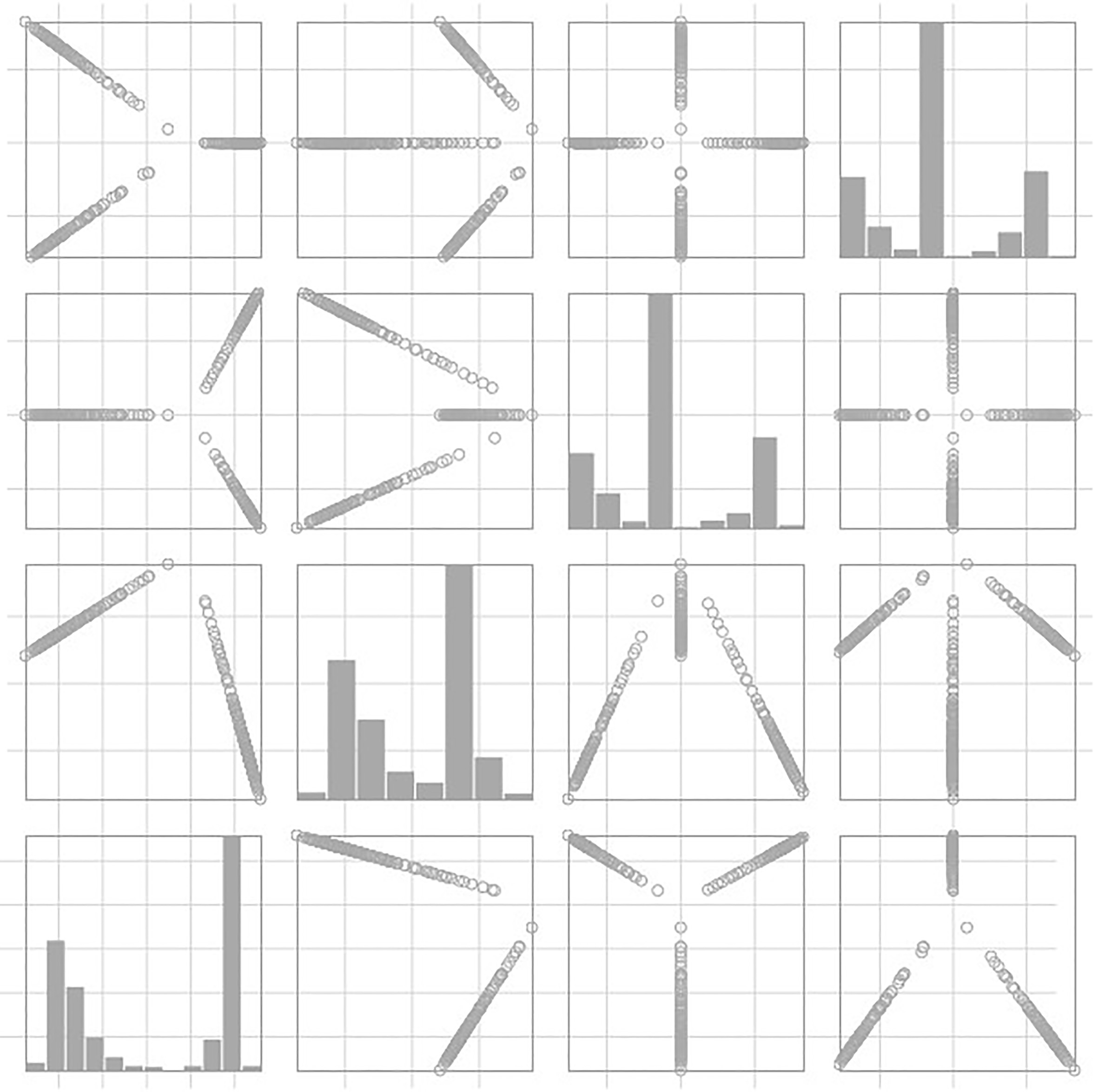
Scatterplot matrix of the latent space obtained with data set synth1 (see description in Table 1). The third and fourth eigenvectors are redundant then, and cluster-specific linear manifolds are rotated in the 2D planes involving the two other dimensions. This still conforms to Proposition 1, and clusters remain easy to delineate in the latent space. However, bimodal distributions would fit poorly to any latent dimension.

The contribution by Xiang and Gong [39] is based on the assumption – not necessarily verified, as shown in Fig. 1 – that each eigenvector should characterize a cluster. This is translated to a greedy search of the latent subspace size, that uses a threshold on the relevance of fitting a bimodal distribution against a single distribution on each dimension of the latent space. This way of proceeding is presented as more robust than expecting a strict fit to a canonical system or analyzing the spectrum, where decisions are not stable enough. The size found for the subspace defines an upper bound to the number of clusters. It is then reduced using BIC [31] as a model comparison criterion.

3. Proposed technique

3.1 A dimensionality-independent gaussian likelihood

The final step of spectral clustering is to apply k-means to the latent representation introduced in Section 2.1. As the model underlying k-means is essentially a Gaussian mixture model (constrained to hard assignments, equal weights and spherical covariance matrices), model selection, i.e., estimating the ground truth number of clusters $K^{*}$ , could in principle be carried out by choosing the $\hat{K}$ that minimizes the BIC criterion [31]:

$\displaystyle\text{BIC}=-2\sum_{n=1}^{N}\log\sum_{k=1}^{K}\omega_{k}\mathcal{N% }(\mathbf{x}_{n}|\mu_{k},\Sigma_{k})+\kappa\log N$ (3)

with mixture weights $\{\omega_{1},\ldots,\omega_{K}\}$ , means $\{\mu_{1},\ldots,\mu_{K}\}$ , covariance matrices $\{\Sigma_{1},\ldots,\Sigma_{K}\}$ , and $\kappa$ the number of parameters in the model, increasing with $K$ . Model selection is then performed by learning mixture models with various $K$ , and selecting the one that minimizes BIC. Basically, as $K$ grows, more components are used to fit the same data, which mechanically increases the associated likelihood, hence decreases the first term in Eq. (3). The optimal model complexity can then be thought as a balance between model fit and complexity.

Minimizing Eq. (3) favors accurate density estimation, which might differ from finding good clustering models, i.e. where components in the mixture are compact and well separated. The Integrated Classification Likelihood (ICL) was introduced in view of this distinction [7]. In the context of k-means, [8] gives a limit formulation of ICL in which the weight vanishes from the first term:

$\displaystyle\text{ICL}=-2\sum_{n=1}^{N}\log\mathcal{N}(\mathbf{x}_{n}|\mu_{% \hat{k}_{n}},\Sigma_{\hat{k}_{n}})+\kappa\log N$ (4)

with $\hat{k}_{n}=\arg\max_{k}{\omega_{k}\mathcal{N}(\mathbf{x}_{n}|\mu_{k},\Sigma_{% k})}{\sum_{j=1}^{K}\omega_{j}\mathcal{N}(\mathbf{x}_{n}|\mu_{j},\Sigma_{j})}$ .

[39] use BIC in a post-processing step. However, in our paper the selection procedure is fully integrated to the problem structure with varying dimensionality as described by Proposition 1. In this context, the mixture model step in the spectral clustering algorithm differs from classical mixture settings by the dimensionality of the latent subspace varying along with the number of components $K$ .

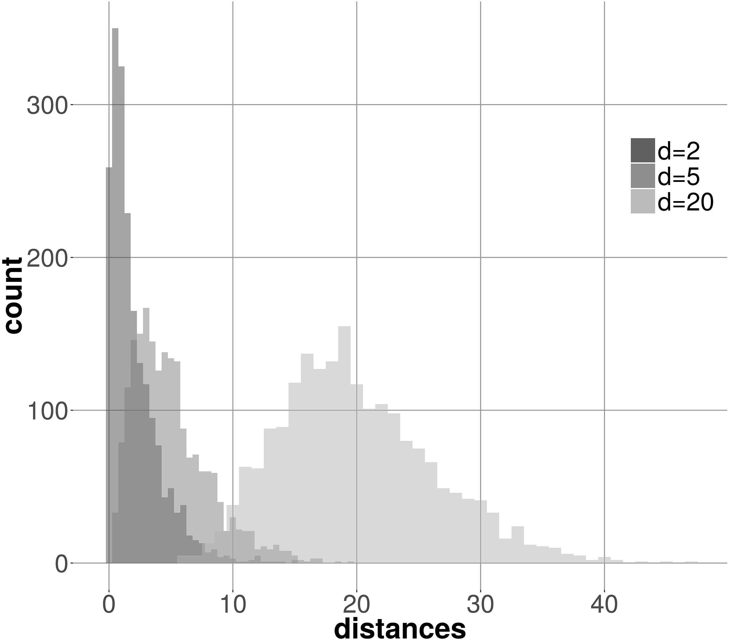
Figure 2 shows the empirical distribution of the square of the Euclidean distance between standard (i.e. $\mathcal{N}(\mathbf{0},\mathbf{I})$ ) $d$ -dimensional Gaussian samples and the origin. Assuming a diagonal covariance with a constant extent (e.g., 1 for $\mathcal{N}(\mathbf{0},\mathbf{I})$ ), it can be seen that this distance squared is expected to increase with $d$ .

Figure 2.

Distributions of the square of the distance between $d$ -dimensional Gaussian samples ( $N=$ 2000) and their respective origin for $d=$ 2 (dark grey), for $d=$ 5 (medium grey) and for $d=$ 20 (light grey).

As the Gaussian density is a function of the square of a distance, according to the observation in Fig. 2 the distribution of its values is influenced by $d$ , the dimensionality of the data. BIC and ICL use the Gaussian density in their first term in Eqs (3) and (4), respectively. In common mixture settings, $d$ is the dimensionality of the initial space, therefore constant, so the dependence goes unnoticed.

Figure 3.

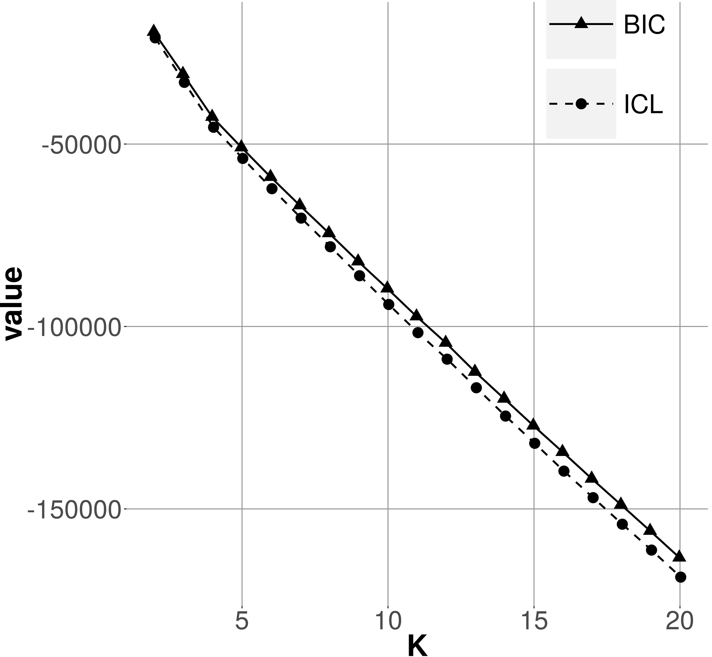
Curves for BIC and ICL criteria as a function of $K$ , with latent representations obtained from the synth1 data generating process. Each value is averaged over 20 independent experiments.

Figure 3 shows the curves for BIC and ICL obtained with latent representations extracted from data generated according to the synth1 process (see definition in Section 4). We see that both criteria are monotonically decreasing functions of $K$ , instead of reaching a minimum at $K=K^{*}=4$ . This discrepancy is a consequence of the latent space dimensionality variation w.r.t. $K$ .

To mitigate this problem, an alternative to the Gaussian density is needed as a plugin to BIC and ICL expressions. We propose a Dimensionality-Independent (DI) likelihood for this purpose:

.

Let $\mathbf{x}\sim\mathcal{N}(\mu,\Sigma)$ . We define the Dimensionality-Independent (DI) likelihood as:

$\displaystyle h(\mathbf{x})=\frac{1}{|\Sigma|^{\frac{1}{2d}}}\exp\biggl{(}-% \frac{1}{2}F^{-1}_{\chi^{2}_{c}}\bigl{(}F_{\chi^{2}_{d}}((\mathbf{x}-\mu)^{T}% \Sigma^{-1}(\mathbf{x}-\mu))\bigr{)}\biggr{)},$ (5)

with $F_{\chi^{2}_{k}}$ the cumulative distribution function of $\chi^{2}(k)$ , $F^{-1}_{\chi^{2}_{k}}$ its quantile function, $d$ the dimensionality of $\mathbf{x}$ and $c$ an arbitrary constant integer.

Let $\mathcal{N}_{1}$ and $\mathcal{N}_{2}$ be two multidimensional Gaussian laws, with means $\mu_{1}$ and $\mu_{2}$ , covariances $\Sigma_{1}$ and $\Sigma_{2}$ , and dimensionalities $d_{1}$ and $d_{2}$ , respectively. Let $\textbf{x}_{1}\sim\mathcal{N}_{1}$ and $\textbf{x}_{2}\sim\mathcal{N}_{2}$ . Let us assume $\Sigma_{1}$ and $\Sigma_{2}$ have equal extent, i.e. $(\prod_{i}\lambda_{1i})^{\frac{1}{d_{1}}}=(\prod_{i}\lambda_{2i})^{\frac{1}{d_% {2}}}=\lambda_{m}$ . Then, if $F_{\mathcal{N}_{1}}(\mathbf{x}_{1})=F_{\mathcal{N}_{2}}(\mathbf{x}_{2})$ , we have $h(\mathbf{x}_{1})=h(\mathbf{x}_{2})$ : in other words, $h$ is insensitive to $d$ , the dimensionality of the data.

The proof can be found in Appendix B. Intuitively, the exponential term in Eq. (5) remaps squared distances of any dimensionality to their counterparts in a common dimensionality $c$ . Corollaries given in Appendix C show that $h$ preserves the order implied by the Gaussian density function over varying dimensionality and extent (see Appendix A for the extent definition).

We explicitly refer to Expression (5) as a likelihood (instead of a density) as it does not integrate to 1 anymore. Appendix D provides empirical evidence of the effectiveness of the proposed likelihood expression. The same evidence also shows that $c$ , the only free parameter in Expression (5), should be set to 2 for reliable model selection: this value is used in the remainder of this paper.

3.2 A novel model selection criterion

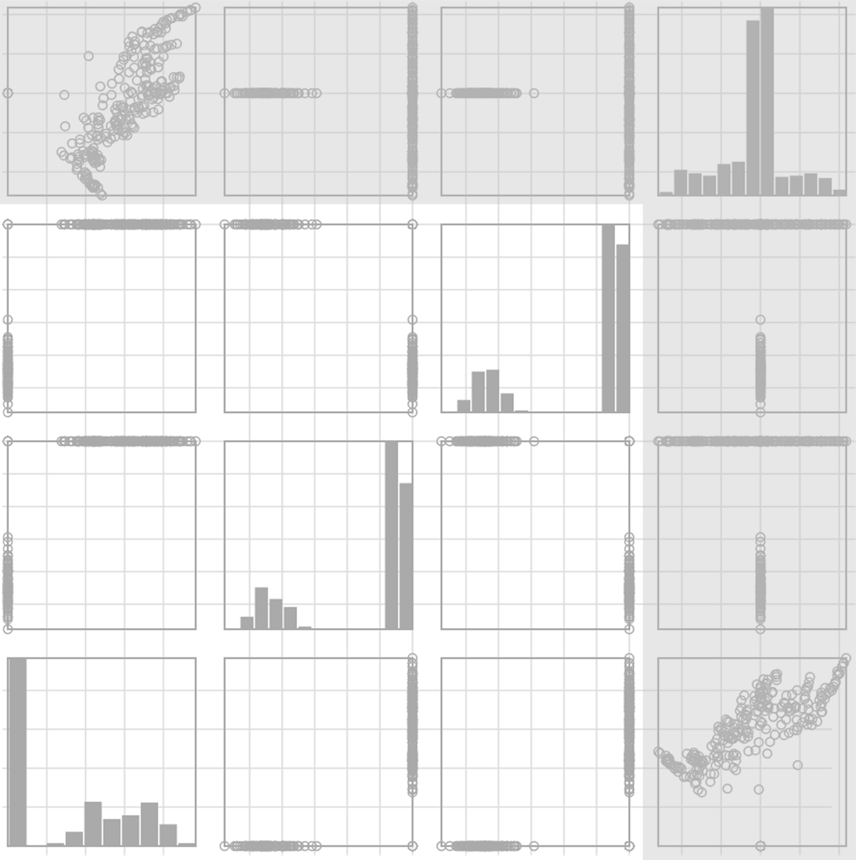
At constant $d$ , the second term in Eqs (3) and (4) favors mixture models with minimal $K$ . However, with spectral clustering, the mixture complexity $K$ is tied to the dimensionality of the latent space (see Section 2.1). In practice, if $K$ is not big enough, then a small number of components does not exhibit satisfactory fit. When $K>K^{*}$ , penalty occurs naturally when spurious dimensions are added to the latent space (see Fig. 4).

Figure 4.

Scatterplot matrix of the latent space obtained with data set synth2 (see description in Table 1). The subspace matching the ground truth number of clusters $K^{*}=3$ is unshaded. Dimensions beyond this subspace (here the $4^{\text{th}}$ is shaded in grey) do not contribute to delineated linear manifolds, leading to poorly fitted mixture models.

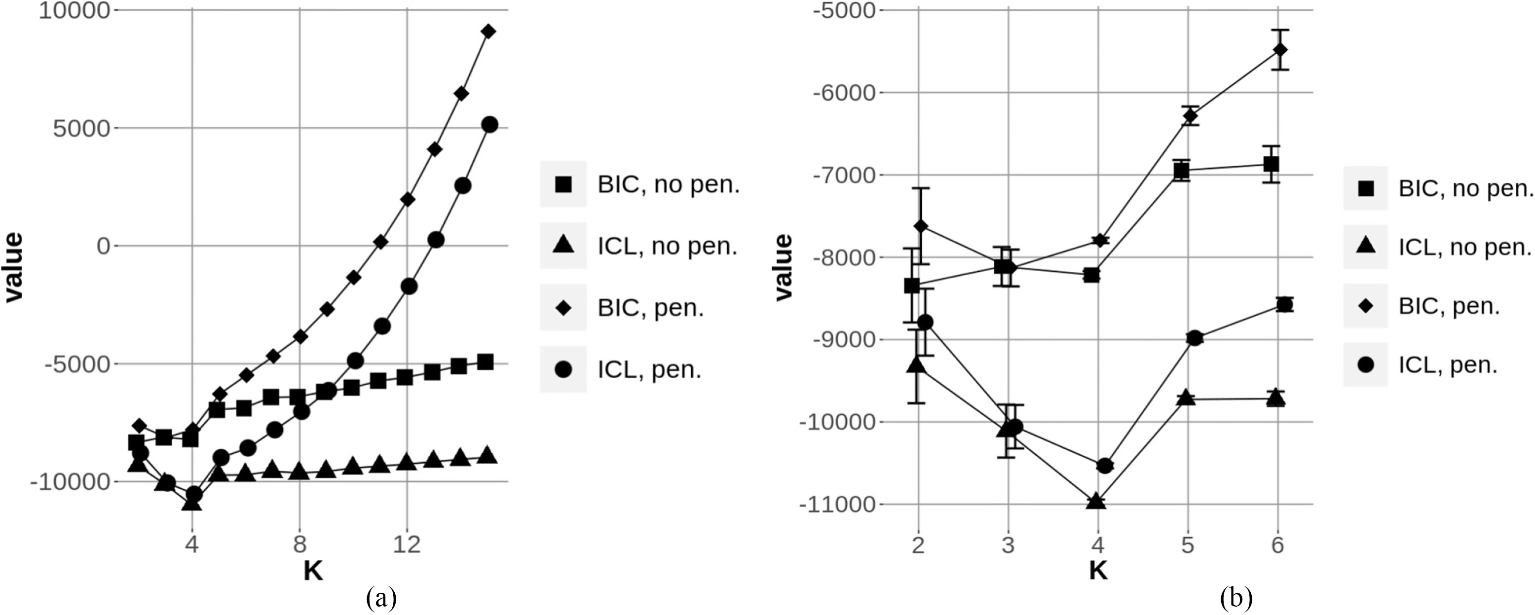
This suggests that a penalty term would be naturally embedded in the spectral clustering model selection problem, possibly leading to the removal of the second term in Expressions (3) and (4). Figure 5 shows the result of experiments mirroring those reported in Fig. 3, when substituting $h$ to $\mathcal{N}$ in Eqs (3) and (4).

Figure 5.

Curves for BIC and ICL criteria as a function of $K$ , with latent representations obtained from the synth1 data generating process. Criteria with or without penalty are considered. Each value is averaged over 20 independent experiments. The curve in a) is magnified for $K\in[2,6]$ in b).

Figure 5a shows the difference between modified criteria, with or without the explicit penalty term. The ground truth for synth1 features 4 clusters (see Section 4), so curves in Fig. 5 are expected to reach a minimum at $K=4$ .

The penalized versions of BIC and ICL exhibit a clear quadratic tendency for higher values of $K$ . This is quite natural, as the number of parameters $\kappa$ in a mixture model grows quadratically with $K$ . Also, we see that criteria without penalty exhibit a linear tendency as $K$ increases: this confirms that the first term in Eqs (3) and (4) already embeds an implicit penalty when using $h$ .

The same curves are magnified for low values of $K$ in Fig. 5b. Error bars reflect the variance of criterion values. Firstly, BIC appears as inadequate for the model selection task at hand, as the criterion values for $K=4$ lie in the confidence intervals for $K=2$ and 3, either with or without the penalty term. This means that depending on the specific generated data set and initialization, $K=2$ or 3 might be selected. For the penalized version of ICL, the value at $K=4$ is also close to the confidence interval for $K=3$ . This leaves the ICL criterion without penalty, for which the optimal value clearly stands out.

Integrating these observations to the ICL criterion in Eq. (4) yields the DI-ICL criterion, that simply maximizes the sum of log-DI-likelihoods of Gaussian components to which data elements are assigned by the k-means procedure:

$\displaystyle\text{DI-ICL}=-2\sum_{n=1}^{N}\log h(\mathbf{x}_{n}|\mu_{\hat{k}_% {n}},\Sigma_{\hat{k}_{n}}),$ (6)

where $\hat{k}_{n}$ is the cluster assignment of element $n$ by k-means. Algorithm 5 uses the DI-ICL criterion in Eq. (6) to cluster a data set, and select the appropriate number of clusters $K^{*}$ automatically, without additional user parametrization.

Leftleft Thisthis Upup UnionUnion FindCompressFindCompress Inputinput Outputoutput A data set $\{\mathbf{x}_{1},\dots,\mathbf{x}_{N}\}$ A set of labels $\{y_{1},\dots,y_{N}\}$ with $y_{i}\in\{1,\dots,K^{*}\}$ $K^{\text{max}}=30$ // $K^{\text{max}}$ is an hard-coded upper bound to $K^{*}$ $\mathbf{S}$ computed according to Eq. (2) $\mathbf{D}$ diagonal computed s.t. $\mathbf{D}_{nn}\leftarrow\sum_{n^{\prime}=1}^{N}{\mathbf{S}_{nn^{\prime}}}$ $\mathbf{U}$ set as solving $\mathbf{U}\Lambda\mathbf{U}=\mathbf{D}^{-\frac{1}{2}}\mathbf{S}\mathbf{D}^{-% \frac{1}{2}}$ $K\leftarrow 2$ $K^{\text{max}}$ $\mathbf{U}_{K}\leftarrow K$ first columns of $\mathbf{U}$ $\{\mu_{1}\dots\mu_{K}\}$ , $\{\Sigma_{1}\dots\Sigma_{K}\}$ $\leftarrow$ sample means and covariances resulting from applying k-means to the $N$ rows of $\mathbf{U}_{K}$ $\text{crit}_{K}\leftarrow$ DI-ICL( $\mathbf{U}_{K},\{\mu_{1}\dots\mu_{K}\},\{\Sigma_{1}\dots\Sigma_{K}\}$ ) according to Eq. (6) $K^{*}\leftarrow\arg\max_{K}$ crit $\{y_{1},\dots,y_{N}\}\leftarrow$ labels resulting from applying k-means with $K=K^{*}$ Spectral clustering with automatic determination of $K^{*}$

4. Experiments

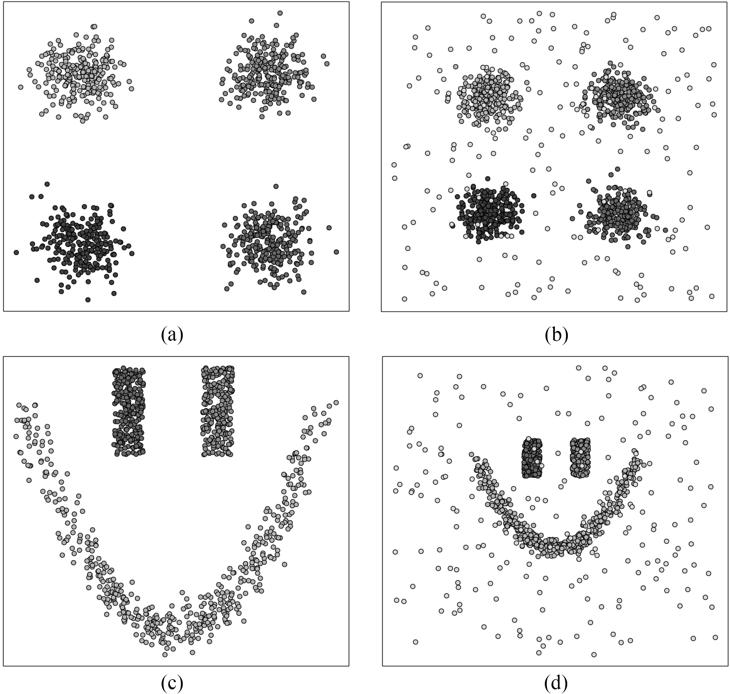
In this study, we introduce synthetic data generating processes synth1 and synth2, that generate noisy replicas of 2D data sets as shown in Fig. 6a and c. Samples of 1000 elements are used in this section. synth1 is the reference case with no specific difficulties for clustering (i.e. well-separated spherical clusters). synth2 is inspired by [42], and features non-convex cluster shapes that k-means or EM typically fail at processing. As means to estimate the impact of background clutter to clustering performance, these synthetic data sets can be augmented by a portion $\alpha\in[0,0.5]$ (i.e. 0 to 500 additional data points), generated from a uniform distribution (see Fig. 6b and d). ISOLET, PENBASED and OPTICAL data sets have been released by [15, 1, 2] respectively. Table 1 summarizes the data sets used to illustrate this study.

Clustering results will be qualified according to the relevance of the estimated $\hat{K}$ , the adjusted Rand index [21], and the Normalized Mutual Information (NMI) [35]. We avoid the use of unsupervised quality indexes (i.e., that do not need the ground truth classes of elements), as they all assume convex clusters. Also, we do not report the purity of obtained clusters, as the clustering error is then under-estimated when the number of clusters is unknown (e.g. 1 cluster per data point yields a purity of 1 in the limit).

Table 1
List of data sets used in the experiments, characterized by their nature, size $N$ , dimensionality $d$ and number of ground truth classes $K$

Name	Nature	$N$	$d$	$K^{*}$
synth1	Synthetic	1000	2	4
synth2	Synthetic	1000	2	3
ISOLET vowels	Real	1800	617	6
PENBASED	Real	10992	16	10
OPTICAL	Real	5620	64	10

Figure 6.

Scatterplots of a) synth1 and c) synth2. The ground truth class of glyphs is emphasized using grey shades. Noisy samples, featuring background clutter, can also be generated for synth1 and synth2 (b and d, respectively).

Although theory expects the alignment of coordinates in the latent space to a basis, in practice linear manifolds are observed irrespective of the Laplacian used (see Figs 1 and 4). As k-means performs badly on ellipsoidal clusters, some authors suggest to normalize the coordinate vectors (i.e., divide coordinate vectors by $\sqrt{\sum_{k=1}^{K}{\mathbf{U}_{nk}^{2}}}$ ), letting clusters concentrate on the expected discrete positions in the latent space [29, 38]. Alternatively we can use the original latent representation without normalizing the coordinate vectors, along with a variant of k-means that estimates ellipsoidal clusters. Elliptical k-means (Ek-means in the remainder) proceeds as the usual k-means, except that a Mahalanobis metric is updated at each step [36] using cluster-wise sample covariances. The distance function for assignments incorporates $\ln|\Sigma_{k}|$ as means to favor clusters with balanced shapes. In practice we found better results when rescaling covariance matrices by $(1/K)\sum_{k=1}^{K}\text{Tr}(\Sigma_{k})$ at each step. Each component is regularized by a prior with large variance, ensuring that DI-ICL is well-behaved when $K>K^{*}$ .

Table 2

Comparative performance of DI-ICL based model selection, with (k-means) or without (Ek-means) coordinate vector normalization. The results are averaged over 20 independent experiments. The performances of ZMP [42] and DBSCAN [17] are also reported. For each metric, the best performing method is bold-faced

		Adjusted rand index
		$\alpha=0.0$	$\alpha=0.1$	$\alpha=0.2$	$\alpha=0.5$
synth1	Ek-means	1.00 $\pm$ 0.00	1.00 $\pm$ 0.00	1.00 $\pm$ 0.00	1.00 $\pm$ 0.00
	k-means	0.99 $\pm$ 0.06	1.00 $\pm$ 0.00	0.97 $\pm$ 0.09	0.98 $\pm$ 0.03
	ZMP	0.97 $\pm$ 0.13	0.92 $\pm$ 0.16	0.80 $\pm$ 0.25	0.73 $\pm$ 0.25
	DBSCAN	0.86 $\pm$ 0.02	0.86 $\pm$ 0.02	0.87 $\pm$ 0.02	0.88 $\pm$ 0.02
		NMI
		$\alpha=$ 0.0	$\alpha=$ 0.1	$\alpha=$ 0.2	$\alpha=$ 0.5
	Ek-means	1.00 $\pm$ 0.00	1.00 $\pm$ 0.00	1.00 $\pm$ 0.00	1.00 $\pm$ 0.00
	k-means	0.99 $\pm$ 0.03	1.00 $\pm$ 0.00	0.98 $\pm$ 0.05	0.98 $\pm$ 0.03
	ZMP	0.99 $\pm$ 0.06	0.95 $\pm$ 0.09	0.89 $\pm$ 0.14	0.84 $\pm$ 0.15
	DBSCAN	0.85 $\pm$ 0.01	0.85 $\pm$ 0.02	0.85 $\pm$ 0.01	0.86 $\pm$ 0.01
		$K^{*}$
		$\alpha=$ 0.0	$\alpha=$ 0.1	$\alpha=$ 0.2	$\alpha=$ 0.5
	Ek-means	4.00 $\pm$ 0.00	4.00 $\pm$ 0.00	4.00 $\pm$ 0.00	4.00 $\pm$ 0.00
	k-means	3.95 $\pm$ 0.22	4.00 $\pm$ 0.00	4.00 $\pm$ 0.00	5.20 $\pm$ 1.54
	ZMP	4.45 $\pm$ 2.01	4.15 $\pm$ 1.09	5.50 $\pm$ 3.99	7.15 $\pm$ 4.93
	DBSCAN	6.80 $\pm$ 1.15	6.75 $\pm$ 1.45	7.30 $\pm$ 1.59	8.50 $\pm$ 1.91
		Adjusted rand index
		$\alpha=$ 0.0	$\alpha=$ 0.1	$\alpha=$ 0.2	$\alpha=$ 0.5
synth2	Ek-means	1.00 $\pm$ 0.00	1.00 $\pm$ 0.00	1.00 $\pm$ 0.00	0.95 $\pm$ 0.16
	k-means	1.00 $\pm$ 0.00	1.00 $\pm$ 0.00	1.00 $\pm$ 0.00	0.95 $\pm$ 0.11
	ZMP	1.00 $\pm$ 0.00	1.00 $\pm$ 0.00	1.00 $\pm$ 0.00	0.98 $\pm$ 0.11
	DBSCAN	0.67 $\pm$ 0.08	0.69 $\pm$ 0.10	0.71 $\pm$ 0.10	0.70 $\pm$ 0.09
		NMI
	$\alpha=$ 0.0	$\alpha=$ 0.1	$\alpha=$ 0.2	$\alpha=$ 0.5
	Ek-means	1.00 $\pm$ 0.00	1.00 $\pm$ 0.00	1.00 $\pm$ 0.00	0.97 $\pm$ 0.10
	k-means	1.00 $\pm$ 0.00	1.00 $\pm$ 0.00	1.00 $\pm$ 0.00	0.97 $\pm$ 0.06
	ZMP	1.00 $\pm$ 0.00	1.00 $\pm$ 0.00	1.00 $\pm$ 0.00	0.99 $\pm$ 0.06
	DBSCAN	0.80 $\pm$ 0.04	0.81 $\pm$ 0.04	0.82 $\pm$ 0.05	0.81 $\pm$ 0.05
		$K^{*}$
		$\alpha=$ 0.0	$\alpha=$ 0.1	$\alpha=$ 0.2	$\alpha=$ 0.5
	Ek-means	3.00 $\pm$ 0.00	3.00 $\pm$ 0.00	3.00 $\pm$ 0.00	3.15 $\pm$ 0.49
	k-means	3.00 $\pm$ 0.00	3.00 $\pm$ 0.00	3.00 $\pm$ 0.00	3.35 $\pm$ 0.93
	ZMP	3.00 $\pm$ 0.00	3.00 $\pm$ 0.00	3.00 $\pm$ 0.00	2.95 $\pm$ 0.22
	DBSCAN	9.10 $\pm$ 1.65	7.90 $\pm$ 1.25	8.15 $\pm$ 1.73	8.45 $\pm$ 1.88

This latter variant is compared to using regular k-means and coordinate vector normalization in a model selection task in Table 2. In the same table we also compare to two reference methods from the literature: one based on spectral clustering by Zelnik-Manor and Perona [42] (referred to as ZMP hereafter1

Implementation available at http://www.vision.caltech.edu/lihi/Demos/SelfTuningClustering.html.

) and DBSCAN, a non-parametric method [17].2

Implementation available at https://cran.r-project.org/web/packages/dbscan/index.html.

Experiments are repeated 20 times for each synthetic data generating process. The same samples are reused for all methods.

In Table 2 we see that Ek-means performs always better than the k-means variant. For both data sets, it is very robust to the addition of background clutter. ZMP yields little improvement to the Ek-means results on synth2, but is highly affected by the addition of clutter in synth1 experiments. Like our Ek-means variant, DBSCAN is not much sensitive to the background clutter, but it heavily overestimates the number of clusters, and yields results consistently worse than all other tested methods. In the remainder, the Ek-means variant is used as the default DI-ICL implementation.

We also apply DI-ICL, ZMP and DBSCAN to the real-world high dimensional ISOLET, PENBASED and OPTICAL data sets. In order also to evaluate the sensitivity of the tested methods, 50% of each data set was subsampled 20 times at random, and fed to DI-ICL, ZMP and DBSCAN. The respective results are averaged, and reported in Table 3.

ZMP and DI-ICL both perform reasonably well on all three data sets. ZMP and DI-ICL both identify the ground truth number of clusters for ISOLET, with a slightly better Rand index and NMI for DI-ICL. $\hat{K}$ is slightly better for DI-ICL on OPTICAL (8.95, against 8.40 for ZMP, when $K^{*}=10$ in this experiment), with also an advantage in terms of Rand index and NMI.

Table 3

Comparative performance of DI-ICL and ZMP on real data sets. Best performing methods are bold-faced for each data set

		Rand	NMI	$K^{*}$
ISOLET	DI-ICL	0.93 $\pm$ 0.02	0.93 $\pm$ 0.01	6.00 $\pm$ 0.00
	ZMP	0.90 $\pm$ 0.02	0.89 $\pm$ 0.01	6.00 $\pm$ 0.00
	DBSCAN	0.11 $\pm$ 0.01	0.37 $\pm$ 0.02	3.80 $\pm$ 0.89
PENBASED	DI-ICL	0.49 $\pm$ 0.02	0.66 $\pm$ 0.01	7.05 $\pm$ 0.22
	ZMP	0.64 $\pm$ 0.04	0.75 $\pm$ 0.02	10.9 $\pm$ 1.07
	DBSCAN	0.30 $\pm$ 0.08	0.64 $\pm$ 0.04	21.0 $\pm$ 2.22
OPTICAL	DI-ICL	0.63 $\pm$ 0.04	0.74 $\pm$ 0.02	8.95 $\pm$ 0.51
	ZMP	0.57 $\pm$ 0.05	0.70 $\pm$ 0.03	8.40 $\pm$ 1.85
	DBSCAN	0.05 $\pm$ 0.05	0.28 $\pm$ 0.16	4.70 $\pm$ 1.56

Figure 7.

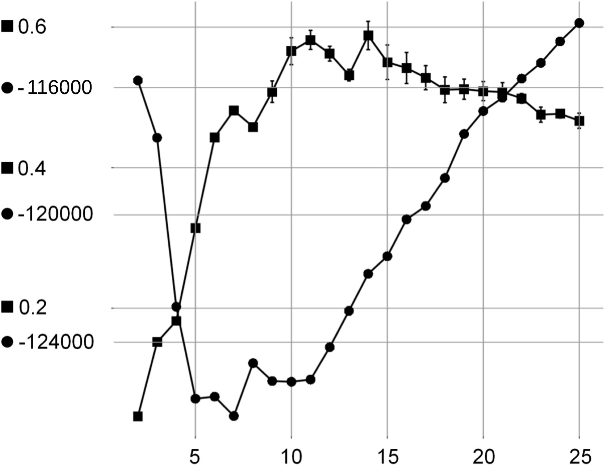
Super-imposed plots of the DI-ICL criterion (discs) and Rand index (squares) w.r.t. $K$ for the PENBASED data set. The displayed values average the results of 20 independent experiments.

Conversely, DI-ICL is outperformed by ZMP for the PENBASED data set, even though the number of clusters and Rand index obtained by DI-ICL are reasonably good. DBSCAN is significantly outperformed by both DI-ICL and ZMP for all data sets, in terms of clustering error and estimated number of clusters. In particular, $K^{*}$ is heavily over-estimated with PENBASED, and under-estimated with ISOLET and OPTICAL.

In Fig. 7, we expand the DI-ICL criterion w.r.t. $K$ for the PENBASED data set. Globally, the graph shows that DI-ICL is fairly well (negatively) correlated to the Rand index. It is thus a reasonable proxy to the clustering error in an unsupervised context. Looking first at the DI-ICL criterion curve, we see that before exhibiting its linear increasing tendency as $K$ grows, the criterion values plateau between $K=$ 5 and 11. Three local minima lie in this interval: at $K=$ 5, 7 and 10. $K=$ 10 is the ground truth for PENBASED. Also, the significant increase of DI-ICL between $K=$ 7 and 8 is exactly associated to a degradation of the Rand index. Hence, beyond merely outputting a point estimate of the selected number of clusters, plotting the DI-ICL curve helps identify a range of satisfactory $K$ values. This can be seen as an improvement over ZMP, that outputs a point estimate for $\hat{K}$ .

5. Discussion

Due to the need to compute the eigenvectors of a square similarity matrix, the naive algorithm is $O(N^{3})$ : it is brought down to $O(N^{2})$ using a Lanczos decomposition method, as clustering generally implies $K<<N$ .

The power iteration algorithm proposes a more efficient decomposition algorithm to tackle this eigenvector analysis [24]. Specifically, they claim that intermediate states of an iterative estimation procedure of the major eigenvector summarize the complete clustering structure, instead of requiring $K$ vectors as in our development. Specifically, Boutsidis et al. show that the power iteration method approximates the major eigenvectors in a meaningful way for k-means [9]. However both contributions do not address the automatic determination of $\hat{K}$ , and the framework developed in our paper is hardly adaptable to their method.

For experiments in this paper a naive implementation has been used, that recomputes k-means afresh for each possible $K$ in a range (typically $[2,30]$ ). Yet the problem has optimal substructure, i.e. up to a rotation factor the $K-1$ first eigenvectors do not depend on the $K^{\text{th}}$ . This feature is used extensively by Lanczos methods [4]. An analogous heuristic could be used in order to speed-up the k-means processes, as the $K-1$ first dimensions of $K-1$ seeds can be initialized with the previous solution.

The eigendecomposition of large matrices can be made even more efficient with the Nyström matrix completion [18]. Approximate similarity computation could also decrease the overall execution time of the algorithm [41]. However potential interactions between these approximation methods and our algorithm should be studied closely.

The Ek-means variant has been established as the best performing option in Section 4. However it has $O(K^{2})$ complexity, when baseline k-means is $O(K)$ . Execution time can then become prohibitive for the highest candidate values for $K$ . This problem could be partly mitigated by exploiting the substructure identified above, or spacing out the covariance matrix updates.

6. Conclusion

From the acknowledged ineffectiveness of classical probabilistic model selection methods in the context of spectral clustering, we derived a Dimensionality Independent Gaussian likelihood expression that restores their applicability. Thorough inspection of the properties of this expression showed that with appropriate parametrization, it yields a relevant model selection criterion.

After experimental validation on synthetic data sets, our method was applied to real-world high-dimensional data sets, and compared to the literature. The proposed technique performs well, and occasionally outperforms the reference methods from the literature. In addition, its probabilistic foundations make it viable for a more qualitative usage, such as identifying a suitable range for $\hat{K}$ rather than a point estimate, as shown by the end of Section 4.

The naive implementation used in the paper has high complexity, but Section 5 highlighted fairly straightforward keys for improvement. Other relevant perspectives certainly lie in combining such spectral clustering schemes with feature selection or metric learning techniques [6]. The proposed criterion and algorithm operate mostly in the latent space of the similarity matrix. Their generality is hence not limited a priori by the similarity function used – chosen as the RBF in Section 2.1. For example, in [39], depending on the data set at hand, experimental results using either the RBF or a similarity function specially adapted to video behavior analysis are given. Experimental confirmation using alternative similarity functions (e.g. cubic, k-NN, exponential) could be part of future work, though.

So far we did not investigate the relative quality of clusters, based on monitoring their shapes and densities. Cluster ranking approaches [5] focus on these features, and will also be considered in future work.

A. Multivariate gaussian properties

Let us recall the expression of the density of the $d$ -dimensional multivariate Gaussian distribution $\mathcal{N}(\mu,\Sigma)$ :

$\displaystyle p(\mathbf{x}|\mu,\Sigma)={(2\pi)^{-\frac{d}{2}}}|\Sigma|^{-\frac% {1}{2}}\exp\left(-\frac{1}{2}(\mathbf{x}-\mu)^{T}\Sigma^{-1}(\mathbf{x}-\mu)\right)$ (7)

In this appendix we investigate how Eq. (7) behaves as $d$ increases. First we focus on the term in the exponent:

.

Let $\mathbf{x}\sim\mathcal{N}(\mu,\Sigma)$ . Then $z=(\mathbf{x}-\mu)^{T}\Sigma^{-1}(\mathbf{x}-\mu)\sim\chi^{2}(d)$ .

Proof..

As $\mathbf{x}\sim\mathcal{N}(\mu,\Sigma)$ , $\mathbb{E}[\mathbf{x}]=\mu$ and $\text{cov}[\mathbf{x}]=\Sigma$ .

$\Sigma^{-1}$ can be factorized using the Cholesky decomposition as $\mathbf{R}^{T}\mathbf{R}$ , with $\mathbf{R}$ an upper triangular matrix. Let $\mathbf{y}=\mathbf{R}(\mathbf{x}-\mu)$ , so that $z=\mathbf{y}^{T}\mathbf{y}$ . The following holds:

$\displaystyle\mathbb{E}[\mathbf{y}]=\mathbb{E}[\mathbf{R}(\mathbf{x}-\mu)]=% \mathbf{R}(\mathbb{E}[\mathbf{x}]-\mu)=\mathbf{0}$ $\displaystyle\text{cov}[\mathbf{y}]=\mathbb{E}[\mathbf{y}\mathbf{y}^{T}]-% \mathbb{E}[\mathbf{y}]\mathbb{E}[\mathbf{y}]^{T}=\mathbb{E}[\mathbf{R}(\mathbf% {x}-\mu)(\mathbf{x}-\mu)^{T}\mathbf{R}^{T}]=\mathbf{R}(\mathbb{E}[\mathbf{x}% \mathbf{x}^{T}]-\mu\mu^{T})\mathbf{R}^{T}=\mathbf{R}\Sigma\mathbf{R}^{T}=% \mathbf{R}(\mathbf{R}^{-1}(\mathbf{R}^{T})^{-1})\mathbf{R}^{T}=\mathbf{I},$

Hence $\mathbf{y}\sim\mathcal{N}(\mathbf{0},\mathbf{I})$ , and $z$ is simply the sum of squares of $d$ independent zero-mean unit-variance Gaussian random variables: in other words $z\sim\chi^{2}(d)$ . ∎

$\mathbb{E}[z]$ and $\text{Cov}[z]$ are $d$ and $2d$ respectively: in other words, the squared Mahalanobis distance of a $d$ -dimensional multivariate Gaussian sample to its respective center appearing in the exponent of Eq. (7) is expected to be $d$ , as perceived intuitively in Fig. 2.

The actual scale and shape of Eq. (7) is controlled by the $|\Sigma|^{-1/2}$ term. Lemma 2 establishes the link between $|\Sigma|$ and $d$ :

.

Let $\Sigma$ be a $d\text{x}d$ positive semi-definite (PSD) matrix. At constant geometric mean of its eigenvalues, $|\Sigma|$ is exponentially increasing with d.

Proof..

Let $\{\lambda_{i}\}_{i\in 1\dots d}$ be the eigenvalues of $\Sigma$ . Then $|\Sigma|=\prod_{i=1}^{d}\lambda_{i}$ . The geometric mean of the $\lambda_{i}$ is defined as $\lambda_{m}=\bigl{(}\prod_{i=1}^{d}\lambda_{i}\bigr{)}^{1/d}$ . We trivially get $|\Sigma|=\lambda_{m}^{d}$ . Setting $\lambda_{m}$ as a constant closes the proof. ∎

$\lambda_{m}$ can be understood as the radius of a hyper-sphere whose volume equals that of the hyper-ellipsoid parametrized by the $\lambda_{i}$ . In this paper, $\lambda_{m}$ is referred to as the extent of the respective component, and serves as basis for comparing models determined on latent subspaces of varying dimension.

B. Proof for the DI likelihood theorem

Proof..

Taking the definition of random variable $z$ from Lemma 1, we have that $z_{1}\sim\chi^{2}_{d_{1}}$ , and $z_{2}\sim\chi^{2}_{d_{2}}$ . Hence, if $F_{\mathcal{N}_{1}}(\mathbf{x}_{1})=F_{\mathcal{N}_{2}}(\mathbf{x}_{2})$ , then a change of variables to polar coordinates yields $F_{\chi^{2}_{d_{1}}}(z_{1})=F_{\chi^{2}_{d_{2}}}(z_{2})$ . Terms within the exponent are then equal.

Lemma 2 established the exponential tendency of $|\Sigma|$ w.r.t. $d$ . Here, we have $|\Sigma_{1}|=\lambda_{m}^{d_{1}}$ and $|\Sigma_{2}|=\lambda_{m}^{d_{2}}$ . Hence the first terms of $h(\textbf{x}_{1})$ and $h(\textbf{x}_{2})$ both equal $1/{\lambda_{m}^{1/2}}$ . The $1/{(2\pi)^{d/2}}$ in Eq. (7) is dropped as it bears no dependence on the data. ∎

C. Corollaries to the DI likelihood theorem

.

Let $\mathcal{N}$ be a multidimensional Gaussian with density $p$ , and $\mathbf{x}_{1},\mathbf{x}_{2}\sim\mathcal{N}$ . If $p(\mathbf{x}_{1})>p(\mathbf{x}_{2})$ then $h(\mathbf{x}_{1})>h(\mathbf{x}_{2})$ . In other words, Theorem 1 preserves the order w.r.t. $p$ .

Proof..

Both $F^{-1}_{\chi^{2}_{c}}$ and $F_{\chi^{2}_{d}}$ in Eq. (5) are monotonically increasing. ∎

.

Let $\mathcal{N}_{1}$ and $\mathcal{N}_{2}$ be two multidimensional Gaussian laws of equal dimensionality, with respective densities $p_{1}$ and $p_{2}$ , and extents $\lambda_{1m}$ and $\lambda_{2m}$ , so that $\lambda_{1m}>\lambda_{2m}$ . We also have $\mathbf{x}_{1}\sim\mathcal{N}_{1}$ and $\mathbf{x}_{2}\sim\mathcal{N}_{2}$ . If $F_{\mathcal{N}_{1}}(\mathbf{x}_{1})=F_{\mathcal{N}_{2}}(\mathbf{x}_{2})$ then $p(\mathbf{x}_{1})<p(\mathbf{x}_{2})$ and also $h(\mathbf{x}_{1})<h(\mathbf{x}_{2})$ . Hence Theorem 1 preserves the order w.r.t. $\lambda_{m}$ .

Proof..

If $F_{\mathcal{N}_{1}}(\mathbf{x}_{1})=F_{\mathcal{N}_{2}}(\mathbf{x}_{2})$ , at constant $d$ Theorem 1 shows terms in the exponent in Eqs (7) and (5) are equal. The order is then fully determined by the $|\Sigma|$ term. ∎

D. Empirical study of the DI gaussian likelihood

In this appendix, we evaluate the ability of Expression (5) to fulfill its intended effect: at constant extent, DI likelihoods of Gaussian samples should be independent of $d$ . To do so we consider a set of dimensionalities taken as $\{2,\dots,10\}$ . In the experiment, this parameter varies jointly with the extent $\lambda_{m}$ in $\{0.5,1,2\}$ and the constant $c$ in $\{1,2,5,10\}$ (defined in Theorem 1, see Eq. (5)). For each possible resulting experimental condition, we sample 1000 data elements from $\mathcal{N}(\mathbf{0},\lambda_{m}\mathbf{I})$ , and compute the associated sum of log-DI-likelihoods using Eq. (5), by analogy to the first terms of the BIC and ICL criteria (Eqs (3) and (4), respectively). The experiment for each condition is repeated 20 times. The joint influence of parameters $d$ , $\lambda_{m}$ and $c$ is investigated with the ANOVA model. Results are displayed in Table 4.

Table 4

Summary of ANOVA applied to sums of log-DI-likelihoods. Joint effects of parameters are also analyzed (lines 4–6). Significance codes: o non-significant, *** high significance

	df	F	p-value	significance
$d$	1	$6.10^{-3}$	0.94	o
$\lambda_{m}$	1	$2.10^{4}$	$<10^{-10}$	***
$c$	1	$9.10^{5}$	$<10^{-10}$	***
$d*\lambda_{m}$	1	0.2	0.63	o
$d*c$	1	0.3	0.61	o
$\lambda_{m}*c$	1	0.2	0.62	o

As expected, log-DI-likelihoods are not affected by the dimensionality $d$ , neither alone nor in conjunction with $\lambda_{m}$ or $c$ . The latter, quite naturally, affect the results ( $p<10^{-10}$ ). However they have independent effects, as $\lambda_{m}*c$ is not significant. Variations in log-DI-likelihoods w.r.t. $d$ are then most likely due to stochastic sampling noise, or in other words, at constant extent the DI-likelihood is insensitive to $d$ .

Let us consider a collection of data items $\{\mathbf{x}_{n}\}_{n=1}^{N}$ so that $\mathbf{x}_{n}\sim\mathcal{N}(\mu,\Sigma)$ . We then study the consistency of the DI-likelihood expression (5), i.e. whether the following implication holds:

$\displaystyle\mathbf{x}_{n}\sim\mathcal{N}(\mu,\Sigma)\implies\operatorname*{% arg\,max}_{\mu}\prod_{n=1}^{N}h(\mathbf{x}_{n})\overset{\scriptscriptstyle N% \rightarrow+\infty}{\rightarrow}\bar{\mathbf{x}}\text{ and }$ $\displaystyle\operatorname*{arg\,max}_{\Sigma}\prod_{n=1}^{N}h(\mathbf{x}_{n})% \overset{\scriptscriptstyle N\rightarrow+\infty}{\rightarrow}\mathbf{S}$

with $\bar{\mathbf{x}}$ and $\mathbf{S}$ the sample mean and sample covariance, respectively, of the $\mathbf{x}_{n}$ . Considering $\mu$ , ideally we would obtain the Maximum Likelihood (ML) estimator via calculus using ${\partial h}/{\partial\mu}=0$ . However closed-form estimators cannot be obtained from Expression (5). Yet we can see that both $F_{\chi^{2}_{d}}$ and $F^{-1}_{\chi^{2}_{c}}$ are strictly increasing functions of $||\mathbf{x}-\mu||$ : hence each $h(\mathbf{x})$ term is maximized by $\mu=\mathbf{x}$ , supporting the relevance of $\bar{\mathbf{x}}$ as the ML estimator of $h$ w.r.t. $\mu$ . For $\Sigma$ , there is no equivalent qualitative argument.

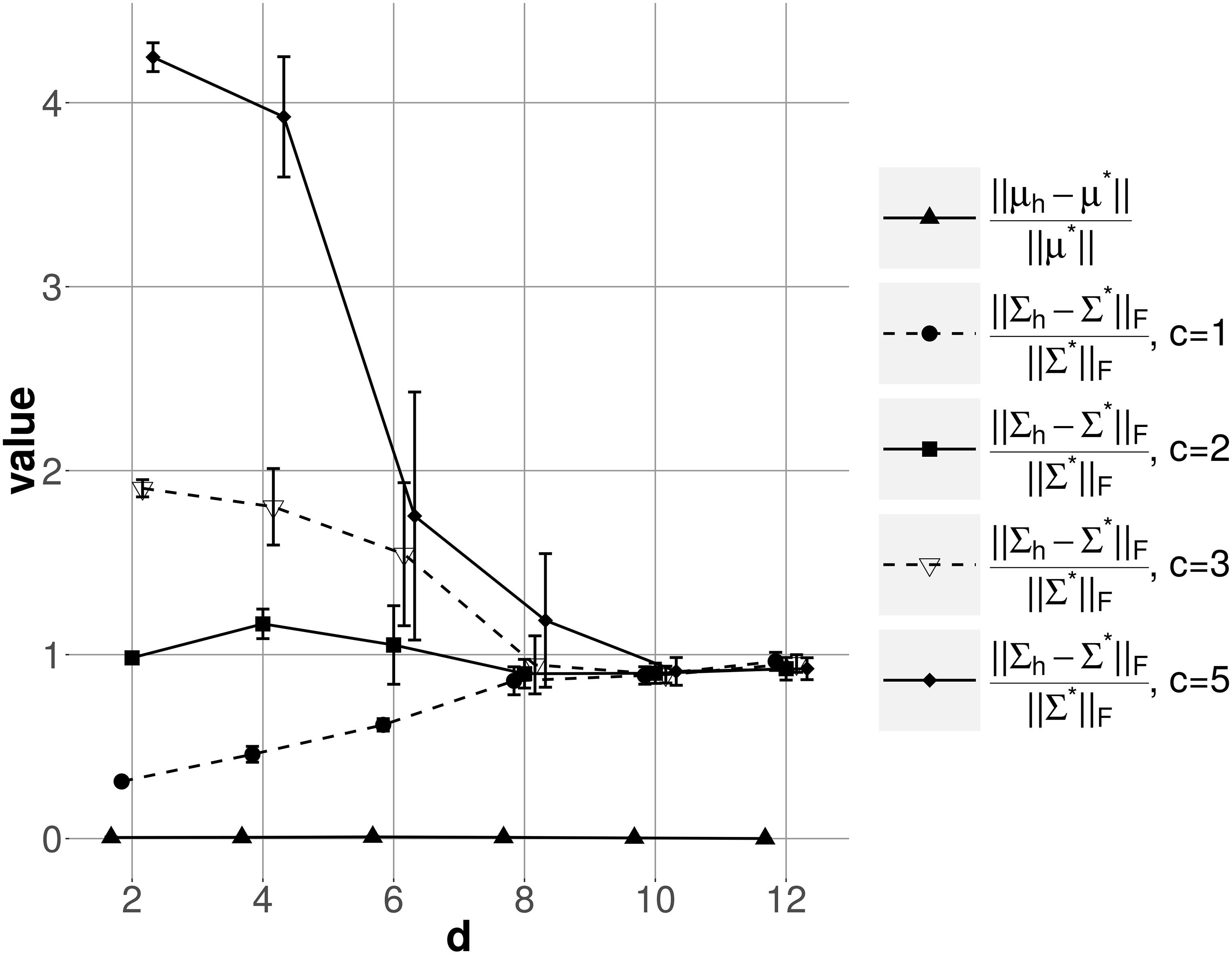
To further investigate the behaviour of $h$ in the context of parameter inference, we perform simulations relying on the numerical optimization of $h(\mathbf{x})$ w.r.t. $\mu$ and $\Sigma$ . The first experiments, reported in Fig. 8, estimate the bias of the ML estimators $\mu_{h}$ and $\Sigma_{h}$ of $h$ for $d$ and $c$ varying in $\{2,\dots,10\}$ and $\{1,2,5\}$ respectively. The true means, denoted as $\mu^{*}$ , are sampled uniformly in an identical range of $[-10,10]$ for all dimensions. The diagonals of the respective $\Sigma^{*}$ are sampled in $[3,5]$ , and off-diagonals in $[-2,2]$ . Even if this process has reasonable chances to yield non-degenerate covariance matrices, a projection on the PSD cone is also performed. They are then rescaled so that their extent equals 1. Each optimization uses sets of 1000 elements sampled independently from $\mathcal{N}(\mu^{*},\Sigma^{*})$ . The experiment for each joint configuration of $d$ and $c$ is repeated 20 times with independent covariance matrices, and averaged in Fig. 8.

Figure 8.

Norm deviations of ML estimators $\mu_{h}$ and $\Sigma_{h}$ w.r.t. $d$ and $c$ . Each measure is obtained by averaging 20 independent simulations. Confidence intervals are reflected by error bars.

In the figure the quality of $\mu_{h}$ is estimated by the scale-corrected deviation in L2-norm ${||\mu_{h}-\mu^{*}||}/$ ${||\mu^{*}||}$ , similarly for $\Sigma_{h}$ and the scale-corrected deviation in Frobenius norm ${||\Sigma_{h}-\Sigma^{*}||_{F}}/{||\Sigma^{*}||_{F}}$ . As expected, the consistency of $\mu_{h}$ is revealed as satisfactory, irrespective of $d$ and $c$ (the curve for $c=2$ is plotted in Fig. 8).

As confirmed by monitoring the respective scale-corrected deviations of $\Sigma_{h}$ , the latter systematically over-estimates $\Sigma^{*}$ . Expression (5) should thus not be used for maximum likelihood estimation of parameters. In Fig. 8 we see that $c$ has an incidence on the variation of this bias w.r.t. $d$ . With $c=$ 1, it is initially small but goes increasing, whereas $c=$ 3 or more yields very high bias for low $d$ . The bias is almost constant with $c=$ 2. However for a model selection purpose, consistency is not needed as long as:

orders induced by Gaussian density $p$ are preserved by respective $h$ . This is guaranteed by Corollary 1 (see Appendix C).

At constant $\lambda_{m}$ and $c$ the bias of $h$ is constant, i.e. orders between models w.r.t. $h$ are preserved over variations of $d$ . Reading Fig. 8, this property is true only for $c=$ 2. This value parametrizes Eq. (5) for the remainder of the paper.

At constant $c$ and $d$ , the bias is constant w.r.t. $\lambda_{m}$ , i.e. model orders w.r.t. $h$ do not depend on model extent. This is guaranteed by Corollary 2 (see Appendix C).

Footnotes

Appendix

References

Alimoglu

and Alpaydin

, Methods of combining multiple classifiers based on different representations for pen-based handwritten digit recognition, In TAINN, 1996.

Alpaydin

and Kaynak

, Cascading classifiers, Kybernetika 34(4) (1998), 369–374.

Attias

, A variational Bayesian framework for graphical models, Advances in Neural Information Processing Systems 12(1-2) (2000), 209–215.

Baglama

and Reichel

, Restarted block Lanczos bidiagonalization methods, Numerical Algorithms 43(3) (2006), 251–272.

Bar-Yossef

Guy

Lempel

Maarek

and Soroka

, Cluster ranking with an application to mining mailbox networks, Knowledge and Information Systems 14(1) (2008), 101–139.

Bellet

Habrard

and Sebban

, A survey on metric learning for feature vectors and structured data, CoRR, abs/1306.6709, 2013.

Biernacki

Celeux

and Govaert

, Assessing a mixture model for clustering with the integrated completed likelihood, IEEE Transactions on Pattern Analysis and Machine Intelligence 22(7) (2000), 719–725.

Bishop

C.M.

, Pattern recognition and machine learning, Springer, 2006.

Boutsidis

Gittens

and Kambadur

, Spectral clustering via the power method – provably, In Proceedings of the 32nd International Conference on Machine Learning (ICML), 2015, pages 40–48.

10.

Bruneau

and Otjacques

, Observations on latent distributions of graph Laplacians, In EGC, 2016, pages 93–104.

11.

Bruneau

Parisot

and Otjacques

, A Heuristic for the Automatic Parametrization of the Spectral Clustering Algorithm, In Proceedings of the 22nd International Conference on Pattern Recognition, 2014, pages 1313–1318.

12.

Cattell

R.B.

, The scree test for the number of factors, Multivariate Behavioral Research 1(2) (1966), 245–276.

13.

Chehreghani

Busetto

and Buhmann

, Information theoretic model validation for spectral clustering, In AISTATS, 2012, pages 495–503.

14.

Comaniciu

and Meer

, Mean shift: A robust approach toward feature space analysis, IEEE PAMI 24(5) (2002). 603–619.

15.

Dietterich

T.G.

and Bakiri

, Error-correcting output codes: A general method for improving multiclass inductive learning programs, In Proceedings of the 9th National Conference on Artificial Intelligence (AAAI), 1991, pages 572–577.

16.

Dupuy

Meignier

Deléglise

and Esteve

, Recent improvements on ILP-based clustering for broadcast news speaker diarization, In Odyssey, 2014.

17.

Ester

Kriegel

Sander

and Xu

, A density-based algorithm for discovering clusters in large spatial databases with noise, In ACM SIGKDD, 1996, pages 226–231.

18.

Fowlkes

Belongie

Chung

and Malik

, Spectral grouping using the Nystrom method, IEEE Transactions on Pattern Analysis and Machine Intelligence 26(2) (2004), 214–225.

19.

Fowlkes

Belongie

and Malik

, Efficient spatiotemporal grouping using the Nyström method, In IEEE Conference on Computer Vision and Pattern Recognition, volume 1, 2001, pages 231–238s.

20.

Frey

and Dueck

, Clustering by passing messages between data points, Science 315(5814) (2007), 972–976.

21.

Gordon

A.D.

, Classification, Chapman and Hall, 1999.

22.

Karatzoglou

Smola

Hornik

and Zeileis

, kernlab – an S4 package for kernel methods in R, Journal of Statistical Software 11(9) (2004), 1–20.

23.

Kohonen

, Essentials of the self-organizing map, Neural Networks 37 (2013), 52–65.

24.

Lin

and Cohen

W.W.

, Power iteration clustering, In Proceedings of the 27th International Conference on Machine Learning, 2010, pages 655–662.

25.

Liu

Latecki

and Yan

, Fast Detection of Dense Subgraphs with Iterative Shrinking and Expansion, IEEE Transactions on Pattern Analysis and Machine Intelligence 35(9) (2013), 2131–2142.

26.

Marlin

B.M.

Kale

D.C.

Khemani

R.G.

and Wetzel

R.C.

, Unsupervised pattern discovery in electronic health care data using probabilistic clustering models, In ACM SIGHIT International Health Informatics Symposium, 2012, pages 389–398.

27.

Nabney

I.T.

, NETLAB: Algorithms for Pattern Recognition, Springer, 2002.

28.

Neal

R.M.

, Markov chain sampling methods for Dirichlet process mixture models, Journal of Computational and Graphical Statistics 9(2) (2000), 249–265.

29.

A.Y.

Jordan

M.I.

and Weiss

, On spectral clustering: Analysis and an algorithm, In Advances in Neural Information Processing Systems, 2002, pages 849–856.

30.

Pieper

Manolakis

Truslow

Cooley

and Lipson

, Performance evaluation of cluster-based hyperspectral target detection algorithms, In Proceedings of the 19th IEEE International Conference on Image Processing, 2012, pages 2669–2672.

31.

Schwarz

, Estimating the dimension of a model, The Annals of Statistics 6(2) (1978), 461–464.

32.

Sheather

S.J.

and Jones

M.C.

, A reliable data-based bandwidth selection method for kernel density estimation, Journal of the Royal Statistical Society B(53) (1991), 683–690.

33.

Shi

and Malik

, Normalized cuts and image segmentation, IEEE Transactions on Pattern Analysis and Machine Intelligence 22(8) (2000), 888–905.

34.

Socher

Maas

and Manning

, Spectral Chinese Restaurant Processes: Nonparametric Clustering Based on Similarities, In AISTATS, 2011, pages 698–706.

35.

Strehl

and Ghosh

, Cluster ensembles-a knowledge reuse framework for combining multiple partitions, JMLR 3 (2002), 583–617.

36.

Sung

and Poggio

, Example-based learning for view-based human face detection, IEEE Transactions on Pattern Analysis and Machine Intelligence 20(1) (1998), 39–51.

37.

van Dongen

, Graph clustering via a discrete uncoupling process, SIAM Journal on Matrix Analysis and Applications 30(1) (2008), 121–141.

38.

von Luxburg

, A tutorial on spectral clustering, Statistics and Computing 17(4) (2007), 395–416.

39.

Xiang

and Gong

, Spectral clustering with eigenvector selection, Pattern Recognition 41(3) (2008), 1012–1029.

40.

Yan

Huang

and Jordan

, Fast approximate spectral clustering, In ACM SIGKDD, 2009, pages 907–916.

41.

Yianilos

P.N.

, Data structures and algorithms for nearest neighbor search in general metric spaces, In Proceedings of the ACM-SIAM Symposium on Discrete Algorithms, 1993, pages 311–321.

42.

Zelnik-Manor

and Perona

, Self-tuning spectral clustering, Advances in Neural Information Processing Systems 17 (2005), 1601–1608.

A probabilistic model selection criterion for spectral clustering

Abstract

Keywords

1. Introduction

1.1 Our contributions

2. Related work

2.1 The spectral clustering algorithm

.

3.1 A dimensionality-independent gaussian likelihood

.

Table 1 List of data sets used in the experiments, characterized by their nature, size N , dimensionality d and number of ground truth classes K

6. Conclusion

A. Multivariate gaussian properties

.

Proof..

.

Proof..

Proof..

C. Corollaries to the DI likelihood theorem

.

Proof..

.

Proof..

D. Empirical study of the DI gaussian likelihood

Footnotes

Appendix

References

Table 1
List of data sets used in the experiments, characterized by their nature, size $N$ , dimensionality $d$ and number of ground truth classes $K$