Feature selection using forest optimization algorithm based on contribution degree

Abstract

As a combinatorial optimization problem, feature selection has been widely used in machine learning and data mining. In this paper, a feature selection method using forest optimization algorithm based on contribution degree is proposed. The proposed method uses a contribution degree strategy which is embedded in forest optimization algorithm. The goal of the contribution degree is to guide the search process of the forest optimization algorithm to select features according to high class correlation and low redundancy between features. The proposed algorithm is verified on some data sets from the UCI repository and the experiments show that the proposed method improves the classification accuracy compared with some other methods.

Keywords

Feature selection forest optimization algorithm contribution degree

1. Introduction

With the development of big data, datasets with a large number of instances and features have brought a great challenges to machine learning. This challenge consists mainly of two aspects: firstly, a large number of redundant and irrelevant features have negative effects on classifier performance [13]. Secondly, calculating a large data set would be time consuming and computationally expensive. Therefore, feature selection is inevitable to deal with this problem by removing irrelevant and redundant features. Feature selection is a common dimensionality reduction technique in many fields such as machine learning, data mining and pattern recognition [18, 31, 12, 6, 38, 43, 49]. The purpose of feature selection is to select salient feature subset and construct the classification model to achieve satisfying prediction accuracy.

Feature selection is usually formulated as a searching optimization problem. For a n-dimension set of feature, there are $2^{n}$ different kinds of structures in the search space. Gheyas and Smith verified that searching the minimal feature subset is an NP problem [16]. In other words, the optimal feature subset can be found by evaluating and enumerating all the possible subsets of features in small datasets. Unfortunately, once the number of features become large in the practical application, the exhaustive search will not be achievable due to the huge computation cost [52]. Therefore, enumeration search methods are impractical for feature selection in large datasets with many features. To overcome this problem, many researchers have attempted to use heuristic algorithms and random search methods to find the optimal feature subset and ideal results have been achieved [53, 10, 7, 35, 44, 15, 51]. Up to now, existing feature selection methods can be classified into filter model, wrapper model, embedded model and hybrid model.

The filter methods use mathematical statistics to analyze the feature set which does not rely on any learning algorithm. The filter-based feature selection methods can be classified into univariate and multivariate methods [5]. In the univariate methods, the relevance of a feature is evaluated individually according to the specific criterion. The univariate algorithms include Information gain [21], Gain Ratio [42], Gini index [20], symmetrical uncertainty [17], Fisher Score (F-Score) [36] and Laplacian Score (L-Score) [46]. The univariate methods do not take the dependencies between the features in the feature selection process into account, and the multivariate approachs are the opposite. Thus, multivariate methods require more computational resources than univariate methods, but their performance is superior to univariate methods. There are numerous well-known multivariate filter methods, such as minimal redundancy-maximal-relevance [14], mutual correlation [27], random subspace method [5] and relevance-redundancy feature selection (RRFS) [2].

The wrapper methods have been widely used since it can achieve higher quality of the feature subsets. Wrapper methods assess the quality of feature subsets by using the classification performance of a specific classifier. The wrapper-based methods can be categorized into sequential and random search methods [28]. The sequential algorithms include Sequential Forward Selection (SFS), Sequential Backward Selection (SBS), sequential forward floating selection (SFFS), sequential backward floating selection (SBFS) and “plus l take away r method” [40]. SFS and SBS are two kinds of hill climbing methods. SFS starts from an empty set of features and at each step a feature is added to the feature set. After meeting the requirement, the feature set obtained is selected as the feature selection result. In fact, at each step of the algorithm, a feature is added to the current set, making the feature selection criterion the largest. The computational complexity of this algorithm is relatively small, but it does not take full account of the correlation between features. But, SBS starts from the full set of features and deletes a feature with the smallest contribution of the evaluation function at each step, until the number of remaining features meet the requirements. Its superiority lies in the full consideration of the relevant characteristics between the features. “plus l take away r method” is actually a compromise between SBS and SFS. Its operation speed is faster than SBS and its operation effect is better than SFS. Moreover, the floating search method uses the floating step to adaptively update the values of l and r. This is a very practical improvement mechanism. On the other hand, the random search method attempts to embed randomness into its search process to avoid local optimal solutions. For example, particle swarm optimization (PSO) [47], genetic algorithm (GA) [37], ant colony optimization (ACO) [33], artificial bee colony (ABC) [11] and forest optimization algorithm (FOA) [26] have been used to solve feature selection problems.

The embedded approach is intended for feature selection as part of the model building process. Thus, the method is associated with a particular learning algorithm, which means that the search for a good subset of features has been performed by a learning algorithm [50]. Support vector machine (SVM) [29], naïve Bayes (NB) [30], and decision tree algorithm [35] are well-known algorithms which are used to construct a learning model in the embedded approach. Therefore, the hybrid model combines a filter and a wrapper model to achieve the best possible performance.

The hybrid model combines the filter and wrapper method together. In the first step, a filter model is applied to reduce the original feature set. Then in the second step, this mode uses wrapper approach to select the optimal feature subset on the reduced feature set. Examples of hybrid approaches include a hybrid genetic algorithm for feature selection wrapper based on mutual information [19], a maximum relevance minimum redundancy feature selection method based on swarm intelligence for support vector machine classification [3] and a filter model for feature subset selection based on genetic algorithm [24].

In general, filter-based methods are usually faster than the wrapper-based ones due to lack of computational cost of the learning model. However, the filter-based methods usually return a relatively low quality. Moreover, the wrapper methods apply a given learning model to evaluate the quality of candidate feature subsets in each iteration. Although the wrapper methods usually achieve better the quality of feature subsets, it needs be at the expense of high computational costs for high dimensional data sets. On the other hand, the goal of the hybrid method is to take advantage of both the filter and the wrapper methods. The embedded approach seeks to subsume feature selection as part of the model building process. In other words, the filter-based feature selection methods usually take the computational time into account. While wrapper, embedded and hybrid approaches are usually concerned with the quality of the selected features. Therefore, a trade-off between these two issues has become an important and necessary goal to providing a good search method.

In this paper, we propose a contribution degree strategy based on forest optimization algorithm, which aims to achieve a high quality approximate solution within an acceptable computational time. We use contribution degree strategy to select some better trees as neighbor trees according to high class correlation and low redundancy between features. This strategy is able to effectively identify and remove the irrelevant and redundant features. We choose features instead of simply sorting the features according to the redundancy of the feature. In the process of searching the optimal solution, we select the features from two aspects: Firstly, in local and global seeding stage, our proposed algorithm randomly will select some features in each iteration. We use normalized mutual information as a metric to assess the correlation between the selected feature and other features. If the correlation is greater than a given threshold (Section 4.1), we consider the feature to be a redundant feature, and the feature will be filtered out. On contrary, we consider this feature as an irrelevant feature that is exactly what we need. For class correlation, if the correlation between the selected feature and class variable is greater than a given threshold, this means that the feature is class correlation, and the feature will be selected. Otherwise, the feature will be discarded. Secondly, In population limited stage, all feature subsets in the forest are sorted by their fitness value. The fitness function assesses the classification accuracy and the quality of the feature subsets. The quality of feature subsets depends on feature redundancy and class correlation. In other words, when the classification accuracy is roughly equal, only those feature subsets whose every feature has higher class correlation and lower redundancy between each other possess higher fitness values. This also means that these feature subsets will not be eliminated. The design of this fitness function removes the irrelevant and redundant features to some extent. In addition, we propose a distance adaptive strategy to effectively and quickly guide the search process to select features according to distance between the current tree and the current global optimal tree. This strategy accelerates the convergence speed of the algorithm. Finally, in order to further improve the performance of the algorithm, we adjust the fitness function. By applying our proposed fitness function, we make sure that each selected feature subset from candidate population satisfies the higher classification accuracy, and ensure that each of their features has higher class correlation and lower redundancy between each other.

The rest of this paper is organized as follows. Section 2 presents related work. Section 3 presents a brief overview of forest optimization algorithm for feature selection. Section 4 presents our method, called FSFOACD. In Section 5 we compare the experimental results of the proposed method to those of other feature selection algorithms. Finally, Section 6 presents the conclusion.

2. Related work

In this paper, the proposed algorithm is a hybrid-based approach. As mentioned above, the goal of the hybrid-based methods is to take advantage of the computational efficiency of the filter model and the proper performance of the wrapper methods. In which, the proposed contribution strategy is the filter model, which is based on information theory. Mutual information as one of filter methods is used to measure the quality of feature by assessing the correlation and redundancy of feature, which possesses a solid theoretical foundation. To date, the combination of mutual information, “relevance” and “redundancy” is widely used for feature selection. For example, Peng et al. [14] used the mutual information as a metric to measure the relationship between the features and class by minimum-Redundancy-Maximum-Relevancy (mRMR) analysis. However, their proposed algorithm is only suitable for interaction between two variables. To identify more complicated variable interactions, some solutions have been proposed. Such as, Bennasar et al. [23] proposed two new feature selection methods based on information theory: Joint Mutual Information Maximisation (JMIM) and Normalised Joint Mutual Information Maximisation (NJMIM). The two methods are designed to address the problem of choosing redundant and irrelevant features in certain circumstance. Vinh et al. [32] proposed a principled approach for deriving new higher-dimensional MI based feature selection approaches by relaxing the identified assumptions, and systematically investigated the issues of employing high-order dependencies for mutual information based features selection. Feature selection based on the relevant redundancy trade-off criteria has become a very popular method in the field of data mining. But the existing feature selection algorithms based on mutual information still have some limitations on common feature selection in practice. This type feature selection methods have the problem of overestimation or underestimation of feature significance. To overcome these limitations, Che et al. [18] proposed a novel mutual information feature selection method based on the normalization of the maximum relevance and minimum common redundancy (N-MRMCR-MI).

On the other hand, Forest optimization algorithm (FOA) is a wrapper model, which was firstly proposed by Ghaemi and Feizi-Derakhshi [26] to solve continuous search space problems. To date, FOA has been applied and developed. For example, Haindl et al. [27] proposed a discrete binary version of the FOA to solve the discrete problems. Yang et al. [37] used FOA to find the best answer for the multidimensional knapsack problem using low number of iterations and low computational effort. Truc [8] used FOA with discrete variables combined with local search to solve the Order Acceptance and Scheduling problem in single-machine environment so that producers gain the maximum profit based on available resources. Moreover, he developed discrete FOA combined with min-max algorithm and local search to solve the independent job scheduling on computational grids with the goal of minimizing makespan[9]. Moreover, FOA is an evolutionary algorithm that has been applied to feature selection. Ghaemi and Feizi-Derakhshi [25] used FOA to cope with discrete search space problems like feature selection and achieved satisfactory results. In addition, he combined FOA with a gradient method to improve the fuzzy c-means (FCM) algorithm [1].

3. Forest optimization algorithm for feature selection

FOA is inspired by the procedure of a few trees in the forests. FOA is an evolutionary algorithm, which is proposed to solve continuous search space problems. Then, FOA is used in discrete search space problems like feature selection. Forest optimization algorithm for feature selection (FSFOA) involves five main stages: (1) initialize trees, (2) local seeding, (3) population limiting, (4) global seeding and (5) update the best tree.

3.1 Initialize trees

The forest is initialized by generating trees randomly. At first, each feature of a tree is randomly generated by ‘0’ or ‘1’. In a dataset with n features, the size of each tree will be ( $n+1$ ) in which one of the features correspond to the “Age” of the tree as in Eq. (1). Each feature equaled ‘1’ indicates that the related feature is selected and each ‘0’ feature means the feature is not selected. The “Age” of each tree is unified to ‘0’. But, in local seeding stage, each iteration of the algorithm will increase the age of all trees except newly generated ones.

$\displaystyle\textit{Tree}=[f_{1},f_{2},f_{3},\ldots,\textit{age}]$ (1)

3.2 Local seeding

Some neighbors of each tree aged 0 are added into the forest in this stage. For each tree aged 0, some features are selected randomly (“Local Seeding Changes” (LSC) parameter determines the number of the selected features and also means the number of neighbor trees to be added). Then, the selected features change to the opposite values. This procedure is considered as local search by adding and removing those features ahead of learning algorithm. Once the local seeding stage finished, the “Age” of each tree except newly generated ones will be added by 1. Figure 1 shows an example of local seeding operator on one tree aged 0, where the dimension of the dataset is 5 and the value of “LSC” is assigned to 2.

Figure 1.

An example of local seeding operation on one tree with “LSC” $=$ 2.

3.3 Population limiting

There are two series of trees that will be omitted from the forest to form the candidate population: (1) trees older than “life time” parameter (“life time” means the maximum allowed “Age” of a tree in the forest) and (2) the extra trees out of the “area limit” parameter after sorted by their fitness value (“area limit” represents the largest number of the trees in the forest). These trees then be migrated to the candidate population and soon afterwards used in global seeding.

3.4 Global seeding

For each selected tree from the candidate population, a set of features are selected randomly (“Global Seeding Changes” (GSC) parameter determines the number of the selected features). Similar to the local seeding, the value of these selected features will be reversed (changing from 0 to 1 or vice versa). But this time, all features are simultaneously considered to be added or deleted and not just one feature at a time. Figure 2 shows an example of global seeding operator on one tree, where the value of “GSC” is assigned to 3.

Figure 2.

An example of global seeding operation on one tree with “GSC” 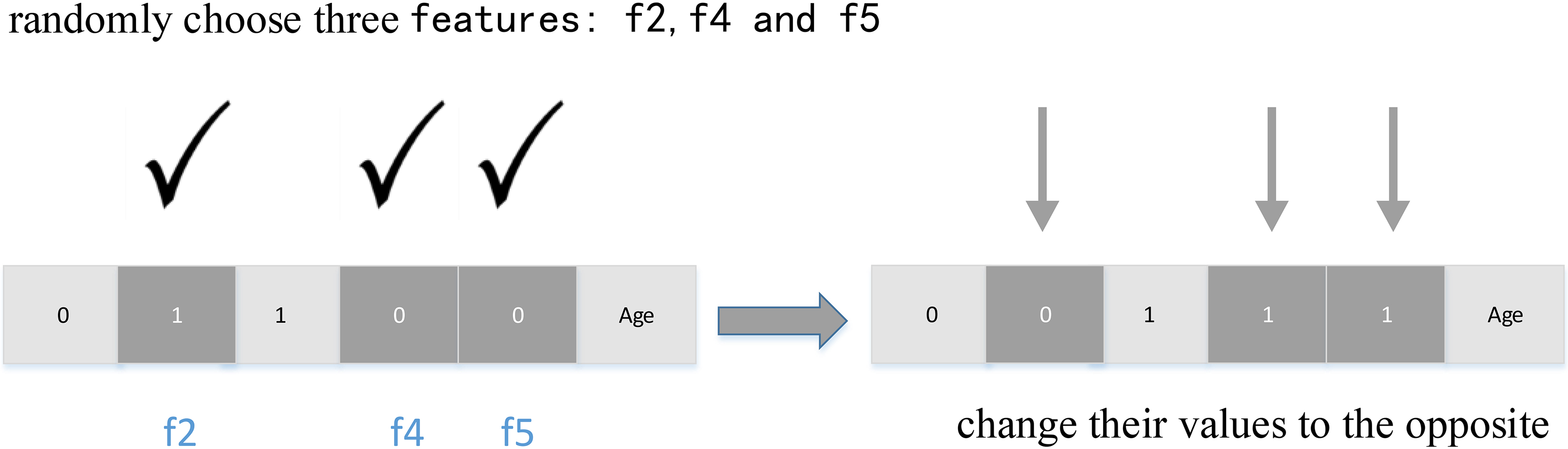$=$ 3.

3.5 Fitness function

The classification accuracy from KNN classifier was selected as the fitness function. For feature selection validation, classification accuracy is an effective measure and it is defined as Eq. (2).

$\displaystyle\textit{CA}=\frac{\textit{the number of correct classifications}}% {\textit{the number of all samples of the dataset}}\times 100\%$ (2)

3.6 Update the best tree

In the last stage, after sorted by the fitness value, the best tree will arise with the highest classification accuracy and its “Age” will be set to ‘0’. The above stages are iteratively performed until the stop condition is satisfied. The pseudo code of FSFOA is illustrated as Algorithm 1.

FSFOA (life time, transfer rate, area limit, LSC, GSC) Input: life time, transfer rate, area limit, LSC, GSC; Output: The best feature set with the highest fitness;[1] Initialize forest with random 0 or 1 trees Each tree is a ( $D+1$ )-dimensional vector $x$ ; (D means the number of all features, the last feature denotes the age of tree) Set the Age of all tree to 0; stop condition is not satisfied Perform local seeding on trees with Age 0; $i=1$ to “LSC” Randomly choose a feature of the selected tree; change from 0 to 1 or vice versa; Increase the Age of all trees by 1. Population limiting. Global seeding. Choose top “transfer rate” percent of trees from the candidate population. each selected tree Choose “GSC” features of the selected tree randomly. change from 0 to 1 or vice versa. Update the best so far tree. Sort trees according to their fitness value. Set the Age of the best tree to 0. Return the best feature subset.

4. Method

Although FSFOA has achieved satisfactory results compared with some other feature selection methods, but there are some shortcomings. Firstly, in local seeding, some features of tree aged 0 are randomly selected and changed and does not consider the class correlation and redundancy between features. Which leads to poor quality of trees in the forest and reduce the search efficiency of FSFOA. Secondly, the number of neighbor trees to be added in each iteration always depends on the number of the features of the dataset and neglects the relationship between the current tree and the current global optimal tree. For some trees close to the optimal tree, adding a lot of neighbor trees will result in a large number of unnecessary calculations and the convergence of the algorithm becomes slower. Thirdly, FSFOA only used the classification accuracy as a fitness function and did not take the contribution of a single feature to the entire feature subset into account. In other words, just using classification accuracy as a fitness function only reflects the performance of the entire feature subset, and cannot reflect the performance of each feature in the feature subset. This deficiency can easily lead to a local optimal solution. In order to solve the above shortcomings, we propose the following solutions.

4.1 Contribution degree

Every mature season in the nature, the grown-up trees produce some seeds that will fall into the mud beside them. Local seeding simulates this process of nature. This operator is mainly manifested in trees with age 0 and adding some neighbor trees around each tree aged 0 in the forest. Due to the limitation of total number of trees, some seeds with enough living space, water, nutrient and sunshine will have a better opportunity to grow up to a young tree. On contrary, they will finally be eliminated in the competition with other seeds. In our work, the neighbor trees are not completely randomly generated any longer, but selected on the basis of how many survival resources they have. The more living resources the tree have, the higher the selected rate will be. Each neighbor tree represents a new location in the feature space. To this end, we propose a contribution degree strategy to assess the quality of the seed. We update the location by choosing one feature of the feature subset and change the value of the feature. The updating formula is as follows:

$\displaystyle f_{i}=\left\{\begin{array}[]{ll}1,&\textit{Sigmoid(contribution}% (f_{i},S))>\textit{rand}\\ 0,&\textit{otherwise}\end{array}\right.$ (3)

$\displaystyle\textit{Sigmoid(x)}=\frac{1}{1+e^{-x}}$ (4)

Where $S$ is a feature subset, ${f_{i}}$ represents the feature of feature subset $S$ that is currently being calculated. Sigmoid(x) is an S-type monotonically increasing function whose value ranges from [0, 1]. We use contribution( ${f_{i}}$ , S) to measure the importance of feature ${f_{i}}$ to all features. Each feature in the optimal feature subset should satisfy minimal redundancy and maximal class relevance. Therefore, a feature with high class correlation and low redundancy between features should have a better opportunity to be selected. Based on this idea, the contribution( ${f_{i}}$ , S) is defined as follows:

$\displaystyle\textit{contribution}(f_{i},S)=C\_\textit{correlation}(f_{i},C)-% \textit{AvgMI}(f_{i},S)$ (5)

Where C_correlation( ${f_{i}}$ , C) is the correlation between feature ${f_{i}}$ and class attribute $C$ . The higher the correlation, the higher the effect of feature ${f_{i}}$ on classification, and vice versa. C_correlation( ${f_{i}}$ , C) is defined as follows:

$\displaystyle\textit{C\_correlation}(f_{i},C)=\textit{MI}(f_{i},C)$ (6)

In Eq. (5), AvgMI( ${f_{i}},S$ ) means the average of the mutual information of the feature ${f_{i}}$ for all the features in the feature subset $S$ . The lower the average mutual information of feature ${f_{i}}$ , the greater the effect of feature ${f_{i}}$ on the feature subset $S$ , and vice versa. AvgMI( ${f_{i}}$ ,S) is defined as follows:

$\displaystyle\textit{AvgMI}(f_{i},S)=\frac{1}{N}\sum_{f_{i}\in S}^{N}\textit{% MI}(f_{i},f_{j})$ (7) $\displaystyle\textit{MI}(F_{i},F_{j})=\sum_{y\in F_{i}}\sum_{x\in F_{j}}p(x,y)% \log\left(\frac{p(x,y)}{p(x)p(y)}\right)$ (8)

Where $N$ is the number of features in the feature subset $S$ . ${f_{i}}$ represents the feature that is currently being calculated. MI( ${F_{i}}$ , ${F_{j}}$ ) means mutual information. ${F_{i}}$ and ${F_{j}}$ represent the value set of ${f_{i}}$ and ${f_{j}}$ , respectively. Mutual information is one of the filter methods used to measure the quality of feature by assessing the correlation and redundancy of feature. Here we use normalized mutual information to measure the relative strength of mutual information and correlation. Mutual information also can be rewritten in terms of entropies and conditional entropies as follows:

$\displaystyle\textit{MI}(f_{i},f_{j})=H(f_{i})-H(f_{i}|f_{j})=H(f_{j})-H(f_{j}% |f_{i})$ (9)

In Eq. (9), ${H(f_{i})}$ and ${H(f_{j})}$ are entropies, and ${H(f_{i}|f_{j})}$ and ${H(f_{j}|f_{i})}$ represent conditional entropies. From Eq. (9), the MI can take values in the following interval:

$\displaystyle 0\leqslant\textit{MI}(f_{i},f_{j})\leqslant\textit{min}\left\{H(% f_{i}),H(f_{j})\right\}$ (10)

From Eq. (10), it follows that the MI between two random variables is bounded above by the minimum of their entropies. Since the entropy between features may vary greatly, this measure should be normalized. Therefore, normalized mutual information is defined as follows:

$\displaystyle\textit{NMI}(f_{i},f_{j})=\frac{\textit{MI}(f_{i},f_{j})}{\textit% {min}\left\{H(f_{i}),H(f_{j})\right\}}$ (11)

In Eq. (11), The NMI is a kind of correlation measure, which takes values in [0,1]. The relative strength of mutual information and correlation can be divided into weakly relevant, relevant and strongly relevant, which is respectively corresponding to the value of NMI belonging to [0, 0.4), [0.4, 0.6) and [0.6, 1] in our method. In feature selection, we are usually interested in features with high class correlation and low redundancy between features. Therefore, only those features whose value of NMI of the C_correlation over 0.6 and value of NMI of the AvgMI below 0.4 have a better opportunity to be selected, and which will be taken into Eq. (5) for calculation. It is worth noting that this assessment is only used for feature selection of local seeding and global seeding stage, and is not used in fitness function calculations.

The additional details of the contribution degree strategy are illustrated with an example as shown in Fig. 3. This strategy is able to effectively identify and remove the irrelevant and redundant features. To a certain extent, we make sure that each tree in the forest selects the features with minimum redundancy while it maximizes the dependency on the target class.

Figure 3.

Illustration of the contribution degree strategy of the proposed method.

4.2 Distance adaptive strategy

In the process of finding the optimal tree, over time, all the trees tend to get closer to the optimal position, eventually, all the trees will remain around the optimal tree. In FSFOA, the number of new neighbor tree added is affected by the “LSC” parameters in local seeding. The “GSC” parameter determines the location of some trees that are migrated to the candidate population and soon afterwards used in global seeding. In each iteration, “LSC” and “GSC” parameters depend on the number of the features of each dataset. Which results in a large number of unnecessary calculations and reduces the efficiency of algorithm search.

In our work, we believe that the number of neighbor trees added in each iteration to find the optimal tree should be related to the distance between the current tree and the current global optimal tree. Therefore, we propose a distance adaptive strategy. We determine the number of neighbor trees to be added based on the distance between the current tree and the global optimal tree. For the trees far from the optimal tree, we need more neighbor trees to speed up space searches. For some tree near by the optimal tree, we only need a small number of neighbor trees to approximate the optimal tree.

The distance here refers to the number of different bits between the current tree and the current global optimal tree. In other words, the “LSC” and “GSC” parameters no longer depend on the number of features of each dataset, but depend on the distance between the current tree and the global optimal tree in each iteration. This distance adaptive strategy can effectively and quickly guide the algorithm to search the optimal tree and accelerate the convergence speed of the algorithm. An illustration of the distance adaptive strategy of the proposed method is shown as Fig. 4. The distance formula is defined as follows:

$\displaystyle\textit{Value}=\textit{distance(Tree, BestTree)}$ (12)

Where Tree means the current tree, BestTree is current global optimal tree. For example, Tree $=$ [1 0 1 0 1 1 0 1 1 1], BestTree $=$ [0 1 0 0 1 1 0 1 1 1]. The distance between the current tree and the global optimal tree is 3. It also means that the current tree needs to add 3 neighbor trees in local seeding stage.

Figure 4.

An illustration of the distance adaptive strategy of the proposed method.

4.3 Improved fitness function

In population limited stage, all trees in the forest are sorted by their fitness value. Then, some trees with the lower fitness value are moved to the candidate population and soon afterwards used in global seeding. Just using classification accuracy as a fitness function only reflects the performance of the entire feature subset, and cannot reflect the performance of each feature in the feature subset. This deficiency is easy to lead to the whole algorithm into the local optimal solution. Therefore, we hope that each feature subset in candidate population satisfies the higher classification accuracy, and ensures that each of their features has higher class correlation and lower redundancy between each other. We define the fitness function as follows:

$\displaystyle\textit{Fitness}=\alpha*\textit{Socres(Tree)}+\beta*\textit{% Accuracy(Tree)}$ (13) $\displaystyle\textit{Scores(Tree)}=\sum_{(f_{i}=1)\in\textit{Tree}}^{N}\textit% {Contribution}(f_{i},S)$ (14)

Where Scores(Tree) is used to measure the importance of the current tree (the current feature subset) by evaluating the correlation and redundancy of each selected feature. Accuracy(Tree) denotes the classification accuracy of the current feature subset on the classifier. $\alpha$ and $\beta$ are two parameters corresponding to the importance of the scores and accuracy, $\alpha$ , $\beta$ $\in$ [0,1] and $\alpha+\beta=$ 1. We have done experiments on the optimal value of $\alpha$ parameter and the related results are presented as Table 2. It can be concluded from Table 2 that the optimal value of $\alpha$ parameter is 0.3. The quality of each tree is evaluated by this fitness function. The purpose of this design is to maximize the fitness value. The details of our FOA-based contribution degree algorithm are provided in Algorithm 2.

[h] FSFOACD (life time, transfer rate, area limit) Input: life time, transfer rate, area limit; Output: The best feature set with the highest classification accuracy; [1] each feature of each tree is initialized randomly by 0 or 1; each tree is composed of (D $+$ 1) dimension vectors; (D means the number of all feature, the last feature denotes the age of tree) Set the Age of tree to 0; stop condition is not satisfied Perform local seeding on trees with Age 0; each tree aged 0 LSC $=$ distance(tree, BestTree); $i$ $=$ 1: LSC Randomly choose a feature $f_{\textit{index}}$ of the tree; $\textit{sigmoid(significance}(f_{\textit{index}},\textit{tree}))>\textit{rand}$ set the value of the $f_{\textit{index}}$ to 1; set the value of the $f_{\textit{index}}$ to 0; Set the Age of tree to 0 and put the tree into forest; The “Age” of each tree except new generated ones will be added by 1; Population limiting; Global seeding; Choose top “transfer rate” percent of trees from the candidate population; tree in selected trees GSC = distance(tree, BestTree); Choose “GSC” features of the current tree randomly; $f_{i}$ in selected features $\textit{sigmoid(significance}(f_{i},\textit{tree}))>\textit{rand}$ set the value of the $f_{i}$ to 1; set the value of the $f_{i}$ to 0; Set the Age of tree to 0 and put the tree into forest; Update the best so far tree; Sort trees according to their fitness value; Set the Age of the best tree to 0; Return the best feature set with the highest classification accuracy;

5. Experiments

In order to verify the efficiency of the proposed method, several experiments are performed on 10 benchmark datasets obtained from the UCI Machine Learning Repository. We compare FSFOACD with several other feature selection algorithms, including Feature selection using Forest Optimization Algorithm(FSFOA)[25], Unsupervised probabilistic feature selection using ant colony optimization (UPFS) [4], Integration of graph clustering with ant colony optimization for feature Selection(GCACO) [34] and Unsupervised FS algorithm based on ACO(UFSACO) [41]. All the experiments are implemented using Matlab on an Intel Core-i3 CPU (2.40 GHz) with 4 GB of RAM. Moreover, in our work, SMO, IBK and J48 in WEKA are embedded into Matlab for implementing SVM, KNN and DT.

Table 1
Characteristics of the datasets used in the experiments

Dataset name	Number of features	Number of classes	Number of instances
Glass	9	7	214
Heart-statlog	13	2	270
Wine	13	3	178
Vehicle	18	4	946
Hepatitis	19	2	155
Parkinsons	23	2	197
Ionosphere	34	2	351
Dermatology	34	6	366
SpamBase	57	2	4601
Sonar	60	2	208

Table 2

Performance evaluation of FSFOACD on the average accuracy of SVM, KNN and J48 classifiers on the whole datasets according to different values of parameter (average over 10 independent runs)

Value of $\alpha$	Accuracy (%)	Value of $\alpha$	Accuracy (%)
0.0	86.12	0.6	83.81
0.1	86.58	0.7	82.92
0.2	84.91	0.8	85.48
0.3	89.21	0.9	82.88
0.4	88.18	1.0	80.43
0.5	85.12

5.1 Datasets

In the experiments, we select several benchmark datasets with different properties to evaluate the performance of the feature selection methods, including Glass, Heart-statlog, Wine, Vehicle, Parkinsons, Ionosphere, Dermatology, SpamBase and Sonar datasets. The datasets can be distributed into three types: small, medium and large in accordance with their feature sizes. In the feature selection problem, the datasets with the number of features belonging to [0, 19], [20, 49] or [50, $\infty$ ] are corresponding to small-scale, medium-scale or large-scale datasets, respectively[22]. Table 1 shows the characteristics of datasets including number of features, number of classes, and number of instances. According to the definition above, Glass, Heart-statlog, Wine, Vehicle and Hepatitis are regarded as the small category. On the other hand, Parkinsons, Ionosphere, Dermatology belong to the medium category. Finally, SpamBase and Sonar are classified into the large category. Among all the data sets, Glass is rather special and is widely used to test the efficiency of feature selection algorithms, which has 9 features, 7 classes and 214 instances. The feature of this data set have certain typicality. Most of the features of this data set are continuous and distributed relatively evenly. Some features of this data set are sparse. The data set has seven class classes, so the dataset can be used for multiclass classification. In this paper, we use classification accuracy as part of the fitness function to evaluate the quality of feature subset, so the multi-class data sets need to be considered. It cannot be ruled out that the attributes in some datasets contain missing values. At this moment, the mean value of available data on corresponding feature can be used to fill in the blank of each missing value.

Table 3
Performance evaluation of FSFOACD on the average accuracy of SVM, KNN and J48 classifiers on the whole datasets according to different values of “area limit”. The value of “life time” and “transfer rate” are considered to 6 and 10%, respectively (average over 10 independent runs)

Area limit	Accuracy (%) standard deviation
30	86.74 $\pm$ 2.73
50	87.23 $\pm$ 1.84
70	85.34 $\pm$ 2.14
90	86.78 $\pm$ 1.07

Table 4

Performance evaluation of FSFOACD on the average accuracy of SVM, KNN and J48 classifiers on the whole datasets according to different values of “transfer rate”. The value of “area limit” and “life time” are considered to 50 and 6, respectively (average over 10 independent runs)

Transfer rate	Accuracy (%) standard deviation
5	88.67 $\pm$ 1.03
10	87.02 $\pm$ 1.12
15	86.91 $\pm$ 2.14
20	87.27 $\pm$ 3.12
25	88.01 $\pm$ 1.44
30	86.24 $\pm$ 1.78

Table 5

Performance evaluation of FSFOACD on the average accuracy of SVM, KNN and J48 classifiers on the whole datasets according to different values of “life time”. The value of “area limit” and “transfer rate” are considered to 50 and 5%, respectively (average over 10 independent runs)

Life time	Accuracy (%) standard deviation
5	87.27 $\pm$ 1.13
10	87.78 $\pm$ 2.18
15	89.19 $\pm$ 1.04
20	86.47 $\pm$ 1.82
25	86.01 $\pm$ 1.64

5.2 Parameter settings

Before conducting the experiment, we need to set the parameters of the proposed method. Based on domain expert experience, the number of trees in the forest is initialized to 30–50, which is satisfied for most data sets [25, 26]. Meanwhile, we have also done experiments to prove this. From the results of experiments in Tables 3 and 4, we find that the values of “area limit” and “transfer rate” have little effect on the performance of our algorithm. The appearance of this phenomenon is understandable. The value of the “transfer rate” parameter indicates that a certain number of trees will be migrated to the candidate population and soon afterwards used in global seeding. The purpose of this operation is to avoid the algorithm to fall into the local optimal solution. The fitness value of these trees is relatively low. So only a relatively small number of these trees need to be added at each iteration of the algorithm. “Life time” means the maximum allowed “Age” of a tree in the forest. Once a tree’s “Age” is greater than the “life time” parameter, it will be omitted is omitted from the forest and added to the candidate population. If we choose a big number for this parameter, the forest will be full of old trees, which will affect the performance of the algorithm. On contrary, if we choose a very small value for this parameter, the trees will get old very soon and they will be eliminated soon. So this parameter affects the performance of the algorithm. We have done experiments on the optimal value of “life time” parameter and the related results are presented in Table 5. In order to reach the best performance, the value of “life time” parameter, “transfer rate” and “area limit” are set to 15, 5% and 50, respectively. The value of “LSC” and “GSC” parameters are no longer determined by the number of the feature of each dataset, but are evaluated by Eq. (12).

Table 6
Average classification accuracy and standard deviation on each dataset using SVM classifier under 10-fold cross validation. The best result for each dataset between all feature selection algorithms is shown in bold face. The last row of the table shows the average value of each algorithm over the whole datasets

Dataset	FSFOACD	FSFOA	UPFS	GCACO	UFSACO
Glass	70.56 $\pm$ 0.01	68.22 $\pm$ 0.14	61.70 $\pm$ 2.22	66.52 $\pm$ 0.82	60.44 $\pm$ 2.58
Heart-Statlog	87.07 $\pm$ 0.03	84.07 $\pm$ 0.74	83.70 $\pm$ 0.89	84.52 $\pm$ 1.42	77.40 $\pm$ 1.46
Wine	99.17 $\pm$ 0.02	96.06 $\pm$ 0.21	93.29 $\pm$ 1.22	94.09 $\pm$ 2.50	94.26 $\pm$ 2.58
Vehicle	80.16 $\pm$ 1.02	62.41 $\pm$ 1.56	63.01 $\pm$ 2.67	70.42 $\pm$ 3.64	61.70 $\pm$ 1.56
Hepatitis	85.26 $\pm$ 0.14	83.46 $\pm$ 0.01	84.46 $\pm$ 1.34	84.52 $\pm$ 2.10	83.25 $\pm$ 1.30
Parkinsons	89.56 $\pm$ 0.01	87.22 $\pm$ 0.04	87.21 $\pm$ 0.01	91.52 $\pm$ 0.43	82.05 $\pm$ 2.30
Ionosphere	95.87 $\pm$ 0.07	94.58 $\pm$ 0.34	86.91 $\pm$ 1.01	90.42 $\pm$ 1.50	87.92 $\pm$ 0.81
Dermatology	98.63 $\pm$ 0.04	96.07 $\pm$ 0.64	97.70 $\pm$ 0.46	95.28 $\pm$ 0.89	95.38 $\pm$ 1.01
SpamBase	92.69 $\pm$ 0.02	88.07 $\pm$ 1.21	88.21 $\pm$ 0.24	88.58 $\pm$ 1.20	87.92 $\pm$ 0.75
Sonar	88.46 $\pm$ 0.03	67.56 $\pm$ 2.20	80.29 $\pm$ 0.32	82.38 $\pm$ 1.40	76.12 $\pm$ 2.40
Average	88.74 $\pm$ 0.139	82.77 $\pm$ 0.71	82.64 $\pm$ 1.03	84.16 $\pm$ 1.59	80.64 $\pm$ 1.67

Figure 5.

The average accuracy of proposed algorithms and other wrapper-based algorithms on the whole datasets using SVM classifier under 10-fold cross validation.

5.3 Results and comparisons

In the experiments, we used different classifiers to evaluate the performance of the proposed method, including k-nearest neighbor (KNN), decision tree (J48) and support vector machine (SVM). In order to obtain fair results, 10-fold cross validation are introduced to measure the accuracy of feature selection algorithms. Tables 6–8 report the average and the standard deviation of classification accuracy over 10 independent runs for FSFOA, UPFS, GCACO, UFSACO and FSFOACD methods using SVM, KNN and J48 classifiers.

Table 7
Average classification accuracy and standard deviation on each dataset using KNN classifier under 10-fold cross validation. The best result for each dataset between all feature selection algorithms is shown in bold face. The last row of the table shows the average value of each algorithm over the whole datasets

Dataset	FSFOACD	FSFOA	UPFS	GCACO	UFSACO
Glass	76.30 $\pm$ 0.07	71.88 $\pm$ 1.56	68.76 $\pm$ 2.37	72.84 $\pm$ 2.91	68.84 $\pm$ 3.83
Heart-Statlog	87.25 $\pm$ 0.05	85.12 $\pm$ 1.28	76.67 $\pm$ 2.25	84.84 $\pm$ 1.32	74.82 $\pm$ 2.87
Wine	98.91 $\pm$ 0.003	98.87 $\pm$ 0.05	96.12 $\pm$ 0.82	93.11 $\pm$ 2.83	93.93 $\pm$ 2.63
Vehicle	78.59 $\pm$ 0.09	73.98 $\pm$ 1.02	65.02 $\pm$ 2.42	74.74 $\pm$ 2.24	68.20 $\pm$ 3.46
Hepatitis	89.20 $\pm$ 0.05	87.09 $\pm$ 1.37	78.71 $\pm$ 0.12	85.84 $\pm$ 1.23	85.90 $\pm$ 1.58
Parkinsons	88.92 $\pm$ 0.19	85.98 $\pm$ 1.28	91.26 $\pm$ 1.07	92.84 $\pm$ 2.14	96.42 $\pm$ 1.33
Ionosphere	93.43 $\pm$ 0.07	92.30 $\pm$ 0.54	89.48 $\pm$ 1.67	89.74 $\pm$ 2.04	86.46 $\pm$ 1.44
Dermatology	99.19 $\pm$ 0.18	97.27 $\pm$ 0.58	97.56 $\pm$ 0.98	95.84 $\pm$ 1.24	93.82 $\pm$ 1.64
SpamBase	93.02 $\pm$ 0.06	89.10 $\pm$ 0.85	89.66 $\pm$ 1.23	88.94 $\pm$ 1.06	85.16 $\pm$ 1.49
Sonar	93.44 $\pm$ 0.12	84.33 $\pm$ 1.86	85.12 $\pm$ 2.58	82.41 $\pm$ 2.14	78.10 $\pm$ 3.67
Average	89.82 $\pm$ 0.08	86.59 $\pm$ 1.03	83.83 $\pm$ 1.55	86.11 $\pm$ 1.91	83.16 $\pm$ 2.39

Table 8

Average classification accuracy and standard deviation on each dataset using J48 classifier under 10-fold cross validation. The best result for each dataset between all feature selection algorithms is shown in bold face. The last row of the table shows the average value of each algorithm over the whole datasets

Dataset	FSFOACD	FSFOA	UPFS	GCACO	UFSACO
Glass	79.07 $\pm$ 0.07	75.71 $\pm$ 1.67	71.15 $\pm$ 2.58	73.13 $\pm$ 1.69	69.10 $\pm$ 3.92
Heart-Statlog	86.29 $\pm$ 0.08	85.15 $\pm$ 0.97	84.15 $\pm$ 1.17	83.13 $\pm$ 1.22	76.10 $\pm$ 4.88
Wine	97.77 $\pm$ 0.03	96.06 $\pm$ 0.24	94.09 $\pm$ 1.47	93.76 $\pm$ 2.87	92.94 $\pm$ 3.11
Vehicle	76.01 $\pm$ 0.04	73.04 $\pm$ 1.09	69.02 $\pm$ 2.78	74.24 $\pm$ 0.93	67.88 $\pm$ 1.98
Hepatitis	89.11 $\pm$ 0.01	86.45 $\pm$ 0.94	86.51 $\pm$ 0.75	84.33 $\pm$ 2.16	83.07 $\pm$ 1.06
Parkinsons	90.89 $\pm$ 0.18	87.91 $\pm$ 1.03	86.95 $\pm$ 2.01	87.43 $\pm$ 1.13	83.10 $\pm$ 2.24
Ionosphere	95.45 $\pm$ 0.09	93.16 $\pm$ 0.67	90.16 $\pm$ 1.04	91.24 $\pm$ 2.01	86.88 $\pm$ 1.56
Dermatology	98.09 $\pm$ 0.12	96.99 $\pm$ 0.87	95.13 $\pm$ 1.23	96.13 $\pm$ 1.56	92.10 $\pm$ 2.91
SpamBase	93.58 $\pm$ 0.17	88.79 $\pm$ 1.89	88.95 $\pm$ 1.57	89.21 $\pm$ 1.01	88.01 $\pm$ 1.22
Sonar	84.20 $\pm$ 0.02	82.69 $\pm$ 0.73	84.09 $\pm$ 1.39	83.27 $\pm$ 0.19	80.60 $\pm$ 1.37
Average	89.04 $\pm$ 0.08	86.59 $\pm$ 1.01	85.02 $\pm$ 1.59	85.58 $\pm$ 1.47	81.97 $\pm$ 2.42

Figure 6.

The average accuracy of proposed algorithms and other wrapper-based algorithms on the whole datasets using KNN classifier under 10-fold cross validation.

Table 6 compares the mean and standard deviation of classification accuracy (average over 10 independent runs) of our proposed FSFOACD method with other wrapper based methods over SVM classifier. It is clear from Table 6 and Fig. 5 that FSFOACD achieved the highest average classification accuracy compared to other feature selection methods on the most of datasets. But for Parkinsons dataset, our proposed algorithm obtained the second place with the classification accuracy of 89.56%, and the GCACO achieved first rank with the classification accuracy of 91.52%. Parkinsons dataset is the only dataset where the difference between the features is extremely small. This makes it difficult to select the proper features for prediction. In addition, our proposed algorithm has significantly improved the accuracy of the classification compared with other algorithms when applied on Vehicle and Sonar datasets.

Figure 7.

The average accuracy of proposed algorithms and other wrapper-based algorithms on the whole datasets using J48 classifier under 10-fold cross validation.

Table 7 reported similar results over the KNN classifier. It can be concluded from Table 7 and Fig. 6 that our proposed FSFOACD method outperforms the other feature selection methods on the most of datasets. For example, for datasets Glass, Heart-Statlog, Wine, Vehicle, Hepatitis, Ionosphere, Dermatology, SpamBase and Sonar, the proposed algorithm returned the highest average classification accuracy. Unfortunately, in the case of Parkinsons dataset, the proposed algorithm did not show good performance. Because as we mentioned before, the difference between the characteristics of the Parkinsons dataset is extremely small, resulting in poor classification. For Glass, Vehicle and Sonar datasets, our proposed algorithm has significantly improvement. It achieved the average classification accuracy 89.82% on all the datasets and lies on the first place among the methods.

Figure 8.

Average classification accuracy on all datasets, with respect to the wrapper-based methods for classifiers SVM, KNN and J48.

Table 8 shows the mean and standard deviation of classification accuracy of the J48 classifier of the proposed algorithm. As can be seen from the Table 8 and Fig. 7, the proposed method achieved the best classification accuracy compared with other methods in each dataset. In addition, the standard deviation of the proposed method is the lowest among all the methods. That means that our proposed method produced robust results. This is due to the fact that the contribution degree strategy of FSFOACD result in selecting more discriminative and high class correlation features and removing irrelevant and redundant features in local and global seeding stage.

Figure 8 provides the average accuracy of SVM, KNN and J48 classifiers on the whole datasets for the proposed algorithm and wrapper-based methods including FSFOA, UPFS, GCACO and UFSACO. For SVM classifier, our proposed method with 0.8874% average accuracy is superior to other methods and the GCACO algorithm obtained 0.8416% average accuracy ranked second. The same result for the KNN and J48 classifiers is shown, where the proposed method outperformed all other algorithms with the average accuracy of 0.8982% and 0.8904%, respectively. While the FSFOA method won the second place with the average accuracy of 0.8659% and 0.8659%, respectively.

6. Conclusion

Feature selection using forest optimization algorithm based on contribution degree was proposed in this paper. This method introduces a contribution degree strategy which is embedded in forest optimization algorithm. The goal of the contribution degree technique is to guide the search process of forest optimization algorithm to select features according to high class correlation and low redundancy between features. To measure performance, SVM, KNN and DT classifiers were applied to some well-known datasets from the UCI repository including Glass, Heart-statlog, Wine, Vehicle, Parkinsons, Ionosphere, Dermatology, Spam Base and Sonar datasets. In addition, the proposed method was compared with some wrapper-based algorithms including FSFOA, UPFS, GCACO and UFSACO. Our results show that the proposed algorithm outperforms those wrapper-based algorithms on 10 benchmark datasets.

Footnotes

Acknowledgments

This work was supported in part by National Science Foundation of China (No. 61572259), supported by the National Social Science Foundation of China (No. 16ZDA054), Special Public Sector Research Program of China (No. GYHY201506080), and was also supported by PAPD.

References

Chaghari

Feizi-Derakhshi

M.R.

and Balafar

M.A.

, Fuzzy clustering based on Forest optimization algorithm, Journal of King Saud University – Computer and Information Sciences 30(1) (2016).

Ferreira

A.J.

and Figueiredo

M.A.T.

, An unsupervised approach to feature discretization and selection, Pattern Recognition 45(9) (2012), 3048–3060.

Unler

Murat

and Chinnam

R.B.

, mr2PSO: A maximum relevance minimum redundancy feature selection method based on swarm intelligence for support vector machine classification, Information Sciences 181(20) (2011), 4625–4641.

Dadaneh

B.Z.

Markid

H.Y.

and Zakerolhosseini

, Unsupervised probabilistic feature selection using ant colony optimization, Expert Systems with Applications 53 (2016), 27–42.

Lai

Reinders

M.J.T.

and Wessels

, Random subspace method for multivariate feature selection, Pattern Recognition Letters 27(10) (2006), 1067–1076.

Pascoal

Oliveira

M.R.

Pacheco

et al., Theoretical evaluation of feature selection methods based on mutual information, Neurocomputing 226 (2016), 168–181.

Paul

Romain

et al., Feature selection for outcome prediction in oesophageal cancer using genetic algorithm and random forest classifier, Compute Med Imaging Graph 60 (2016), 42.

Truc

DV.

, Enhancing forest optimization algorithm for order acceptance and scheduling, Proceedings of the Asia Pacific Industrial Engineering & Management Systems Conference, 2015.

Truc

DV.

, Using discrete forest optimization algorithm for independent jobs scheduling on computational grids with local search, Proceedings of the Asia Pacific Industrial Engineering & Management Systems Conference, 2015.

10.

Hancer

Xue

and Karaboga

et al., A binary ABC algorithm based on advanced similarity scheme for feature selection, Applied Soft Computing 36(0)(2015), 334–348.

11.

Zorarpacı

and Özel

S.A.

, A hybrid approach of differential evolution and artificial bee colony for feature selection, Pergamon Press, Inc. 2016.

12.

Miao

and Pedrycz

, Granular multi-label feature selection based on mutual information, Elsevier Science Inc, 2017.

13.

Chandrashekar

and Sahin

, A survey on feature selection methods, Pergamon Press, Inc. 2014.

14.

Peng

Long

and Ding

, Feature selection based on mutual information: Criteria of max-dependency, max-relevance, and min-redundancy, IEEE Computer Society, 2005.

15.

Wang

and Niu

, A novel bacterial algorithm with randomness control for feature selection in classification, Neurocomputing (2017), 228.

16.

Gheyas

I.A.

and Smith

L.S.

, Feature subset selection in large dimensionality domains, Pattern Recognition 43(1) (2010), 5–13.

17.

Biesiada

and Duch

, Feature selection for high-dimensional data – a pearson redundancy based filter, Advances in Soft Computing 45 (2007), 242–249.

18.

Che

Yang

et al., Maximum relevance minimum common redundancy feature selection for nonlinear data, Information Sciences (2017), 409.

19.

Huang

and Rong

, A hybrid genetic algorithm for feature selection based on mutual information, Pattern Recognition Letters 28(13) (2007), 1825–1844.

20.

Raileanu

L.E.

and Stoffel

, Theoretical comparison between the gini index and information gain criteria, Annals of Mathematics & Artificial Intelligence 41(1) (2004), 77–93.

21.

and Liu

, Feature selection for high-dimensional data: A fast correlation-based filter solution, Twentieth International Conference on International Conference on Machine Learning, AAAI Press, 2003, pp. 856–863.

22.

Tahir

M.A.

Bouridane

and Kurugollu

, Simultaneous feature selection and feature weighting using Hybrid Tabu Search/-nearest neighbor classifier, Pattern Recognition Letters 28(4) (2007), 438–446.

23.

Bennasar

Hicks

and Setchi

, Feature selection using Joint Mutual Information Maximisation, Expert Systems with Applications 42(22) (2015), 8520–8532.

24.

Elalami

M.E.

, A filter model for feature subset selection based on genetic algorithm, Knowledge-Based Systems 22(5) (2009), 356–362.

25.

Ghaemi

and Feizi-Derakhshi

M.R.

, Feature selection using forest optimization algorithm, Pattern Recognition 60 (2016), 121–129.

26.

Ghaemi

and Feizi-Derakhshi

M.R.

, Forest Optimization Algorithm, Expert Systems with Applications 41(15) (2014), 6676–6687.

27.

Haindl

Somol

Ververidis

et al., Feature selection based on mutual correlation, Lecture Notes in Computer Science, 2006.

28.

Kabir

M.M.

Shahjahan

and Murase

, A new local search based hybrid genetic algorithm for feature selection, Neurocomputing 74(17) (2011), 2914–2928.

29.

Pal

and Foody

G.M.

, Feature selection for classification of hyperspectral data by SVM, IEEE Transactions on Geoscience & Remote Sensing 48(5) (2010), 2297–2307.

30.

Friedman

Geiger

and Goldszmidt

, Bayesian network classifiers, Machine Learning 29(2–3) (1997), 131–163.

31.

Hoque

Bhattacharyya

D.K.

and Kalita

J.K.

, MIFS-ND: A mutual information-based feature selection method,Expert Systems with Applications 41(14)(2014), 6371–6385.

32.

Vinh

N.X.

Zhou

Chan

et al., Can high-order dependencies improve mutual information based feature selection? Pattern Recognition 53 (2016), 46–58.

33.

Castillo

Soria

Melin

et al., New approach using ant colony optimization with ant set partition for fuzzy control design applied to the ball and beam system,Information Sciences 294 (2015),203–215.

34.

Moradi

and Rostami

,Integration of graph clustering with ant colony optimization for feature selection, Knowledge-Based Systems 84 (2015), 144–161.

35.

Shunmugapriya

and Kanmani

,A hybrid algorithm using ant and bee colony optimization for feature selection and classification (AC-ABC Hybrid), Swarm & Evolutionary Computation, 2017, 36.

36.

and Han

, Generalized fisher score for feature selection, Twenty-Seventh Conference on Uncertainty in Artificial Intelligence, AUAI Press, 2011, pp. 266–273.

37.

Yang

Wang

Xiao

et al., Feature selection using a combination of genetic algorithm and selection frequency curve analysis, Chemometrics & Intelligent Laboratory Systems 148 (2015), 106–114.

38.

Sheikhpour

Sarram

M.A.

Gharaghani

et al., A survey on semi-supervised feature selection methods, Pattern Recognition 64(2) (2016), 141–158.

39.

Mahmoudi

and Lailypour

, A discrete binary version of the forest optimization algorithm, International Conference on Information Technology, Computer & Communication, 2015.

40.

Moustakidis

S.P.

and Theocharis

J.B.

, SVM-FuzCoC: A novel SVM-based feature selection method using a fuzzy complementary criterion, Pattern Recognition 43(11) (2010), 3712–3729.

41.

Tabakhi

Moradi

and Akhlaghian

, An unsupervised feature selection algorithm based on ant colony optimization, Engineering Applications of Artificial Intelligence 32(6) (2014), 112–123.

42.

Mitchell

T.M.

, Machine learning, McGraw-Hill, NewYork, 1997.

43.

Wang

Tang

et al., LED: A fast overlapping communities detection algorithm based on structural clustering, Neurocomputing 207 (2016), 488–500.

44.

Zhang

Cao

et al., KDVEM: A k-degree anonymity with vertex and edge modification algorithm, Computing 97(12) (2015), 1165–1184.

45.

Sugumaran

Muralidharan

and Ramachandran

K.I.

, Feature selection using decision tree and classification through proximal support vector machine for fault diagnostics of roller bearing, Mechanical Systems & Signal Processing 21(2) (2007), 930–942.

46.

Cai

and Niyogi

, Laplacian score for feature selection, International Conference on Neural Information Processing Systems, MIT Press, 2005, pp. 507–514.

47.

Liu

and Shang

, A fast wrapper feature subset selection method based on binary particle swarm optimization, Evolutionary Computation, IEEE, 2013,, pp. 3347–3353.

48.

Farzi

and Rezazadeh

, A new forest optimization algorithm for solving multidimensional knapsack problem, The International Conference in New Research of Industry & Mechanical, 2015.

49.

Tang

et al., An efficient and scalable density-based clustering algorithm for datasets with complex structures, Neurocomputing 171 (2016), 9–22.

50.

Saeys

Inza

and Larrañaga

, WLD: Review of feature selection techniques in bioinformatics, Bioinformatics 23(19) (2007), 2507–2517.

51.

Xue

Jiang

Zhao

et al., A self-adaptive artificial bee colony algorithm based on global best for global optimization, Soft Computing 8 (2017).

52.

Zhang

Gong

et al., Feature selection algorithm based on bare bones particle swarm optimization, Neurocomputing 148(1) (2015), 150–157.

53.

Beheshti

and Shamsuddin

S.M.

, A review of population-based meta-heuristic algorithm, International Journal of Advances in Soft Computing & Its Applic 5(1) (2013), 1–35.

Feature selection using forest optimization algorithm based on contribution degree

Abstract

Keywords

1. Introduction

2. Related work

3. Forest optimization algorithm for feature selection

3.1 Initialize trees

3.4 Global seeding

4. Method

4.1 Contribution degree

Table 1 Characteristics of the datasets used in the experiments

Footnotes

Acknowledgments

References

Table 1
Characteristics of the datasets used in the experiments