A framework for generating condensed co-location sets from spatial databases

Abstract

Spatial co-location mining is a useful tool for discovering spatial association patterns of feature sets which are frequently observed together in nearby geographic space. Most of co-location mining techniques aim to find all prevalent co-located feature sets which satisfy a given prevalence threshold. However the result is often large, especially when the prevalence threshold is set low, or long co-location patterns present. Moreover the output has many redundant information which makes it difficult for users to filter useful patterns. This work introduces the problem of mining reduced sets of co-location patterns in order to concisely represent interesting spatial relationship patterns. With aiming two such outputs in the form of maximal and closed co-locations, this paper proposes an algorithmic framework to discover maximal co-location patterns and closed co-location patterns as well as all prevalent co-location patterns, and presents the algorithm details for each pattern discovery. The developed algorithms are correct and complete in finding maximal co-locations and closed co-locations. The experiment result shows that the framework reduces candidate feature sets effectively and finds co-location patterns efficiently.

Keywords

Spatial association pattern mining condensed patterns maximal co-location closed co-location

1. Introduction

The evolution of location sensing, wireless networks and ubiquitous computing is generating large quantities of rich spatial data with geographic references. Spatial data mining has been used for extracting interesting, previously unknown, and potentially useful patterns or knowledge from large spatial databases [26, 28, 11, 7]. In spatial data analysis, spatial proximity is an important concept to determine spatial dependencies or spatial auto correlations among objects since nearby objects are more related than distant objects [32, 28]. As family of spatial data mining, co-location mining has been used to uncover implicit spatial dependency patterns from large spatial datasets.

Given a data set of spatial objects, where each object is presented with a tuple $<$ feature type $f$ , instance $i d$ , location ( $x$ , $y$ ) $>$ , spatial co-location mining problem is to discover all subsets of features which are frequently observed together in nearby areas [29]. For example, in Fig. 1a, each data point is represented by its feature type and instance id, e.g., A.1. The data points may represent the locations of local stores/facilities, plant species, or crime instances in the area. In Fig. 1b, identified neighboring objects are connected by a dotted line. We can notice that objects of features A, B, and C often make neighbor relationships. For example, {A.2, B.4, C.2} and {A.3, B.3, C.1} are the co-location instances of {A, B, C}. The strength of a co-location pattern is measured using the prevalence metric such as participation index [29]. If the prevalence value of a co-located feature set is greater than a given prevalence threshold, the feature set becomes a co-location pattern.

Figure 1.

Spatial data and neighbor relationships.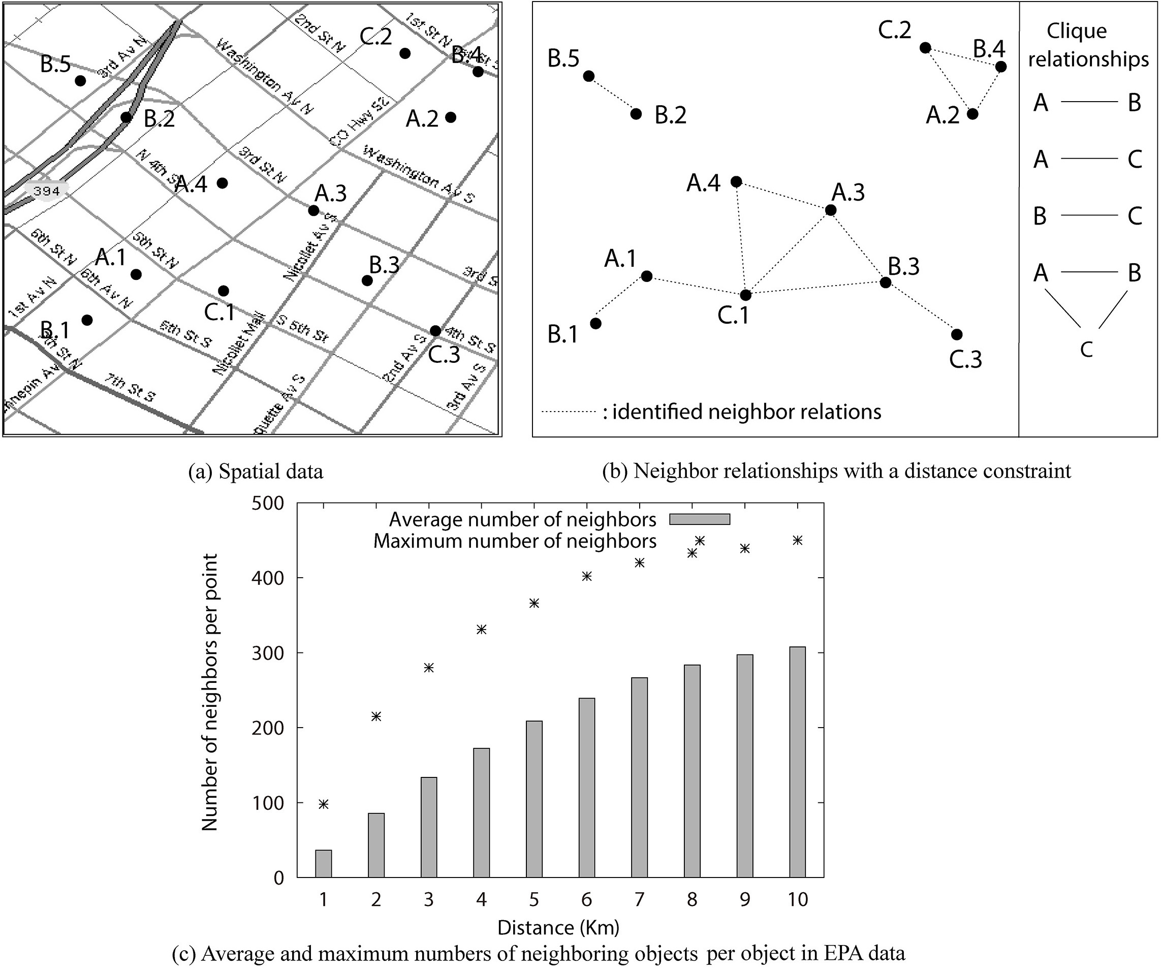

Spatial co-location mining is useful in many application domains including geographic information systems [17], public safety [19], public health [6], ecology [30], agriculture [36], social science [35], environmental science [3, 20], Earth science [9], criminology [24, 18], urban planning [16, 21], and business [23, 42]. For example, co-located plant species discovered from plant distribution data sets can contribute to plant geography and phytosociology study. As another application, consider location-based services. Finding what services are frequently requested by users in geographic proximity is an interesting problem. For example, consider an E-commerce service company which provides different types of services, such as weather, movie timetabling, ticketing and parking queries [23]. The requests for those services may be sent from different locations by mobile users. The service provider may be interested in discovering types of services that are requested by geographically neighboring users, in order to provide location-sensitive advertisement and recommendation. For instance, having known that ticketing requests are frequently asked close to timetabling requests, the provider may choose to advertise the ticketing service to all customers that ask for a timetabling service.

Spatial co-location mining is a computationally expensive and resource intensive task. Figure 1c shows the average and maximum numbers of neighbor objects per object by different neighbor distances, with the facility data of two counties from the Environmental Protection Agency (EPA) databases [1]. It is computationally expensive to search all possible co-location instances directly from such dense spatial data sets. Moreover, the number of co-located feature sets discovered is often large, especially when the prevalence threshold is set low, or when there exist long patterns present in the spatial neighborhoods. A length $l$ co-location pattern with $l$ features implies the presence of additional $2^{l}-l-1$ co-location patterns as well, with being explicitly examined during the mining process. In addition, the complete set of co-location patterns has many redundant information, which makes it difficult for users to filter useful patterns from it. Therefore, reducing the number of output patterns is desirable for the understandability of the mining result as well as the computation cost.

This work studies the problem of finding compact sets of co-location patterns in order to concisely represent interesting relationship patterns in spatial data. We adopt relevant models from frequent itemset mining literature [12], and present the compact representation of co-location patterns with the terms of maximal and closed co-locations. A maximal co-location is a prevalent co-located feature set for which none of its immediate supersets are prevalent. The result of maximal co-location discovery makes the smallest output of co-location mining from which all co-location patterns can be derived. They are useful for spatial datasets which have long length co-location patterns; however maximal co-locations lead to a loss of information since the prevalence values of all co-locations cannot be specified with the maximal result set. In contrast, the output of closed co-locations provides the minimal representation of co-located feature sets that preserves the prevalence information of all co-location patterns.

The contributions of this paper are summarized like following: First, we introduce the problem to find the compact representation set of co-location patterns with maximal co-locations or closed co-locations. Second, we aim to develop an algorithmic framework which can discover maximal co-locations and closed co-locations as well as all prevalent co-located feature sets. The common mining procedures of three different outputs are identified for the framework. Third, two algorithms, MaxColoc and ClosedColoc, for mining maximal co-locations and closed co-locations, respectively, are developed on the framework. The proposed algorithms adopt several schemes for reducing the number of candidate sets examined, efficiently searching their co-location instances, and effectively determining the maximality or closeness of a prevalent co-located feature set. Forth, we prove that the proposed algorithms are correct and complete in finding maximal co-locations and closed co-locations. Moreover they are experimentally evaluated with real data and synthetic data. The experiment result shows that the framework reduces candidate feature sets effectively and finds maximal co-location and closed co-location patterns efficiently.

The remainder of the paper is organized as follows. Section 2 begins with an introduction to the traditional co-location model, and defines maximal co-location and closed co-location patterns for the compact representations of co-locations. Section 3 describes an algorithmic framework for mining maximal and closed co-locations as well as all prevalent co-located feature sets. Section 4 presents the MaxColoc algorithm and ClosedColoc algorithm. The analysis of the proposed algorithms is given in Section 5. The experimental results are presented in Section 6. In Section 7, we conclude this paper by discussing related work and future work.

2. Co-location patterns

This section describes key terms used in co-location mining, and then gives the formal definitions of maximal co-locations and closed co-locations.

2.1 General co-location semantics

Let a set of $m$ spatial features be $F=\{f_{1},\ldots,f_{m}\}$ and a set of their instance objects be $S=S_{f_{1}}\cup\ldots\cup S_{f_{m}}$ , where $S_{f_{i}}$ is a set of objects whose feature type is $f_{i}$ , $1\leqslant i\leqslant m$ . An object $o_{i}\in S$ is represented with a tuple $<$ feature type $f$ , instance $i d$ , location ( $x$ , $y$ ) $>$ . Let $R$ be a neighbor relationship over the locations of objects in $S$ . When Euclidean metric is used for the neighbor relationship $R$ , two objects, $o_{i},o_{j}\in S$ , are neighbors each other when the distance between them is not greater than a given distance threshold $d$ ; that is, $R(o_{i},o_{j})=$ true $\Leftrightarrow$ Euclidean distance $(o_{i},o_{j})\leqslant d$ . We assume that the relationship $R$ is symmetric and reflexive.

.

Co-location instance: A set of spatial objects, $I=\{o_{1},\ldots,o_{l}\}\subseteq S$ , is the co-location instance of a feature set $X=\{f_{1},\ldots,f_{l}\}\subseteq F$ , if (1) $I$ contains an object of each feature in $X$ , i.e., $o_{i}\in S_{f_{i}}$ , and (2) all objects in $I$ are neighbors each other, i.e., $R(o_{i},o_{j})=$ true for $1\leqslant i<l$ , $i<j\leqslant l$ .

For example, in Fig. 2a, {A.2, B.4, C.2} is a co-location instance of {A, B, C} because the instance includes objects of the three features, A, B and C, and they are neighbors each other. A co-location instance with $l$ features is called a length $l$ co-location instance. We also call co-location instances to clique instances.

Figure 2.

Co-locations, closed co-locations, and maximal co-locations.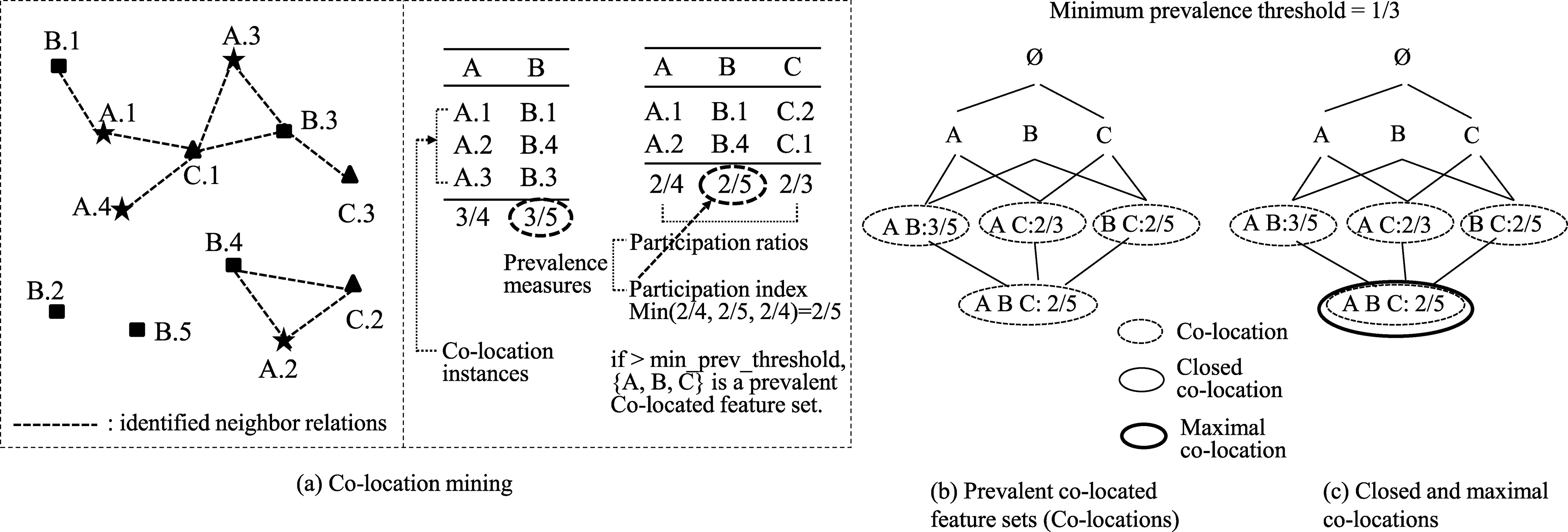

The prevalence strength of a co-location pattern is often measured with participation ratio and participation index [29].

.

Prevalence measure: The participation index $PI(X)$ of a co-located feature set $X=\{f_{1},\ldots,f_{l}\}$ is defined as $PI(X)=\min_{f_{i}\in X}\{PR(X,f_{i})\}$ , where $PR(X,f_{i})$ is the participation ratio of feature $f_{i}$ in $X$ . The participation ratio of feature $f_{i}$ in $X$ , $PR(X,f_{i})$ , is the probability that $f_{i}$ presents in the neighborhood of co-location instances of $X\setminus\{f_{i}\}$ , i.e., $PR(X,f_{i})=\frac{\textit{Number of distinct objects of }f_{i}\textit{ in co-location instances of }X}{\textit{Number of objects of% }f_{i}}$ , $1\leqslant i\leqslant l$ .

Participation index measure indicates wherever a feature $f_{i}$ in $X=\{f_{1},\ldots,f_{l}\}$ is observed, with a probability of at least $PI(X)$ , all the other features in $X$ are observed in its neighborhood. For example, with the data of Fig. 2a, compute the prevalence value of a feature set {A, B, C}. The example shows two co-location instances of {A, B, C}. They are {A.2, B.4, C.2} and {A.3, B.3, C.1}. The participation ratio of feature A in $X=$ {A, B, C}, $P R$ ( $X$ , A), is $\frac{2}{4}$ since among total four objects of feature A in the example, only A.2 and A.3 are included in the co-location instances. In the same way, $P R$ ( $X$ , B) is $\frac{2}{5}$ and $P R$ ( $X$ , C) is $\frac{2}{3}$ . Thus, the participation index of $X$ , $PI(X)$ , is $\min$ { $P R$ ( $X$ , A), $P R$ ( $X$ , B), $P R$ ( $X$ , C)} $=$ $\frac{2}{5}$ .

.

Co-location: A co-located feature set $X=\{f_{1},\ldots,f_{l}\}$ , $l\geqslant 2$ is a prevalent co-located feature set (co-location pattern), if the participation index value of $X$ satisfies a minimum prevalence threshold, $\theta$ , that is, $PI(X)\geqslant\theta$ .

2.2 Co-location models for reduced sets

The closed co-location and maximal co-location patterns we propose are defined as following:

.

Closed co-location: A prevalent co-located feature set $X$ is a closed co-location if there is no proper super set $X^{\prime}\supset X$ such that $PI(X^{\prime})=PI(X)$ .

A closed co-location is a prevalent co-located feature set if none of its immediate supersets has exactly the same prevalence value as it. For example, in Fig. 2, when the minimum prevalence threshold $\theta$ is 0.2, {A, B}, {A, C} and {A, B, C} are closed co-locations. {B, C} is prevalent but not a closed co-location because its participation index value is the same as its superset {A, B, C}.

.

Maximal co-location: A prevalent co-located feature set $X$ is a maximal co-location if no super set of $X$ is prevalent, i.e., for $X^{\prime}\supset X$ , $PI(X^{\prime})<\theta$ , where $\theta$ is a minimum prevalence threshold.

A maximal co-location is a prevalent co-located feature set that does not appear as a subset of other co-location patterns. For example, in Fig. 2c, only {A, B, C} is a maximal co-location.

3. Algorithmic framework

Co-location pattern discovery is challenging because spatial objects are distributed on continuous space, and share complex spatial relationships with each others [28]. A large fraction of the computation time in mining co-location patterns is devoted to finding co-location instances. This section presents an algorithmic framework to efficiently discover maximal and closed co-location patterns as well as all prevalent co-located feature sets. The framework focuses on reducing the number of candidate sets examined, efficiently searching their co-location instances, and effectively checking the maximality or closedness of prevalent co-locations. Figure 3 shows the framework proposed with main components.

Figure 3.

An algorithmic framework of mining co-location patterns.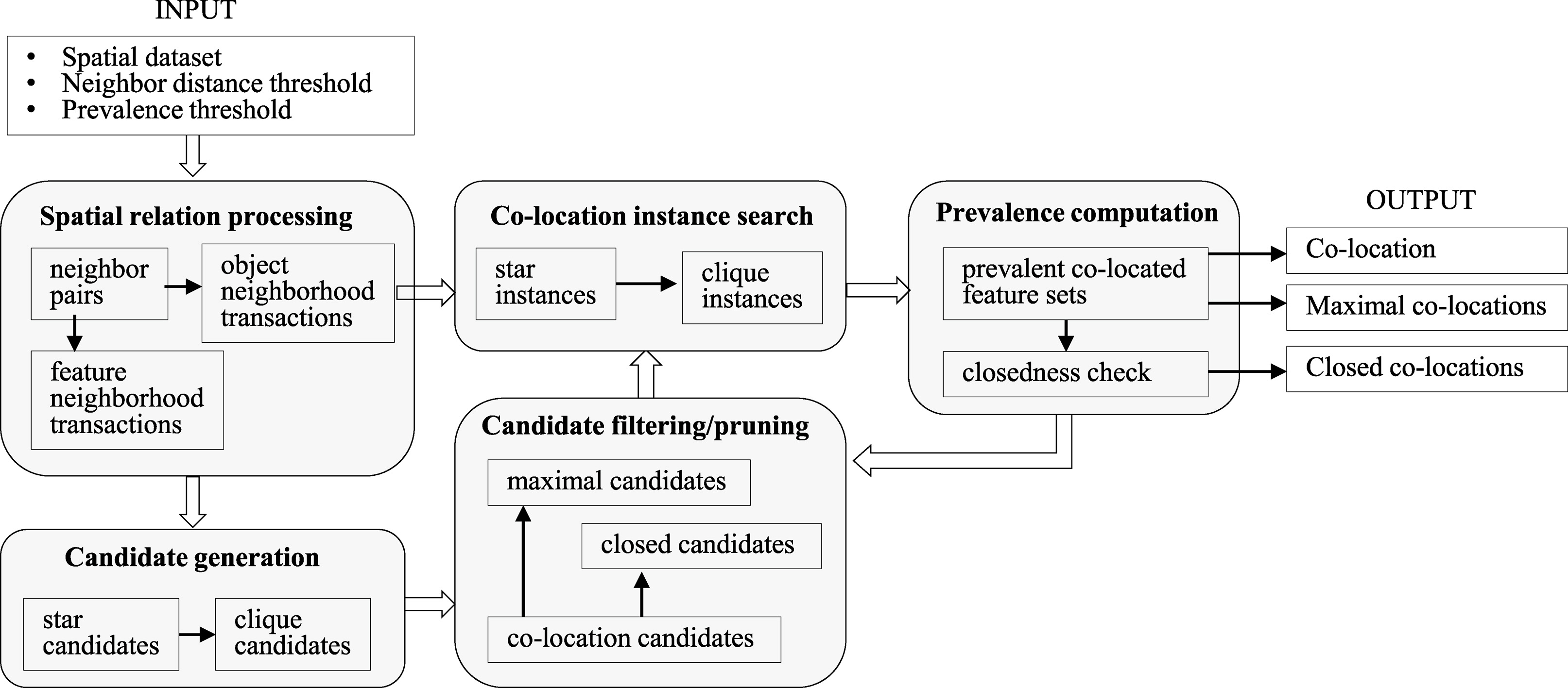

3.1 Spatial relationship preprocess

As pointed out by Shekhar and Chawla [28], the cost of fully exploring a spatial dataset for finding all co-location instances having clique neighbor relationships can, in some cases, be more expensive than co-location pattern search. Our framework adopts the idea of neighborhood materialization [41] in order to effectively handle spatial relations for co-location mining, but organize spatial relations in two different data structures: feature neighborhood transaction record, and neighborhood transaction record. Feature neighborhood records are used for generating candidate co-located feature sets. Neighborhood records are used for finding potential co-location instances.

Given a set of spatial features $F=\{f_{1},\ldots,f_{m}\}$ and a set of their instance objects $S=S_{f_{1}}\cup\ldots\cup S_{f_{m}}$ , where an object $o_{i}\in S$ is represented with a tuple $<$ feature type $f$ , instance $i d$ , location ( $x$ , $y$ ) $>$ , the data structures are defined like following:

.

The feature neighborhood transaction record of an object of feature $f$ , $o\in S_{f}$ , is defined to $ft_{f}(o)=$ { $f$ , $E$ } where $f$ is the feature of the reference object $o$ and $E\subseteq F\setminus\{f\}$ is a set of distinct features of objects which have neighbor relationships with $o_{i}$ .

The feature neighborhood transaction of each object gives the information of other features presented in its neighborhood area. In the example with Fig. 4a, $ft_{c}$ (C.1) is {C, A, D, E} because A.1, D.2 and E.1 are neighbors of the reference object, C.1. The set of feature neighborhood transactions of all objects of feature $f$ , $FT(f)=$ { $ft_{f}(o_{1}),\ldots,ft_{f}(o_{k})$ }, is called a $f$ -feature neighborhood transaction set. As shown in Fig. 4b, the $C$ -feature neighbor transaction set $F T$ (C) is { $ft_{c}$ (C.1), $ft_{c}$ (C.2), $ft_{c}$ (C.3)}.

Figure 4.

Different data structures to store spatial neighbor relations.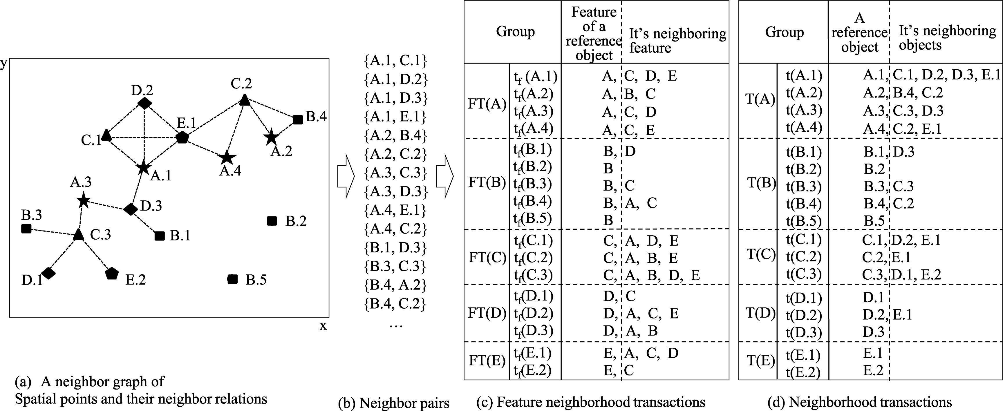

.

The neighborhood transaction record of an object $o\in S$ , $t(o)$ , is defined to $t(o)=$ { $o$ , $J$ } where $J=$ { $o_{i}|o_{i}\in S$ , $o$ .feature $<o_{i}$ .feature, and $R(o_{i},o)=$ true}.

We assume there is a total ordering of feature types, such as lexicographic. The neighborhood transaction informs conditional neighboring objects presented in the neighborhood of each object. For example, in Fig. 4c, the neighborhood transaction record of C.1, $t$ (C.1), is {C.1, D.2, E.1}. Although A.1 is a neighbor of C.1, A.1 is not included in $t$ (C.1) because the feature type of A.1 is not greater than the feature type of C.1 in a lexicographical order (i.e., A $\ngtr$ C). In fact, the relation between A.1 and C.1 is already reflected in the neighborhood transaction of A.1. Therefore this data structure can store all neighbor relations without duplication. The set of neighborhood transactions of objects of feature $f$ is called a $f$ -neighborhood transaction set $T(f)=\{t(o_{1}),\ldots,t(o_{k})\}$ .

Algorithm 1 shows the pseudo code of the spatial relation processing. All neighboring object pairs can be found using a geometric method such as plane sweep [5], a spatial range query method using quaternary trees or R-trees [28]or a grid-based neighbor search [43]. We use a plane sweep algorithm [5] for neighbor pair search (Line 1 in Algorithm 1) because as argued in [15], it might be more beneficial to operate on raw spatial data than spatial query methods which requires building indexes especially for the operation. The neighborhood transactions are simply generated by grouping the neighboring objects per each object and checking the condition of the neighborhood transaction by Definition 7 (Line 2 in Algorithm 1). The feature neighborhood transactions are also generated by grouping the neighboring objects per each object, extracting distinct feature types from them according to Definition 6 (Line 3 in Algorithm 1).

Algorithm 1 Algorithm for neighborhood preprocess
Input
$F=\{f_{1},\ldots,f_{m}\}$ : a set of distinct spatial features
$S$ : a spatial dataset
$d$ : a neighbor distance threshold
Output
$N P$ : a set of all neighbor pairs.
FNT: a set of feature neighborhood transaction records.
$N T$ : a set of neighborhood transaction records.
Neighborhood preprocess
1) $NP=$ find_neighbor_pairs ( $S$ , $d$ );
2) $\textit{FNT}=$ gen_feature_neighborhood_transactions ( $N P$ , $F$ );
3) $NT=$ gen_neighborhood_transactions ( $N P$ , $F$ );

3.2 Candidate generation

The search space of co-location patterns has 2 ${}^{m}-m-1$ candidates, where $m$ is the number of features. The number of candidates is exponentially increased with increase of features. Therefore rather than identifying all instances of candidates, our framework filters out false candidates, i.e., candidates that are not patterns, without identifying all of their instances. We use a divide-and-conquer approach, which first divides feature transaction records by reference features, generates potential candidate feature sets per reference feature from them, and then generates true co-location candidates with combining them. The following details the candidate generation process. Algorithm 2 shows the pseudo code.

Algorithm 2 Algorithm for candidate generation
Input
$F=\{f_{1},\ldots,f_{m}\}$ : a set of spatial features
$\theta$ : a minimum prevalence threshold
Output
$C$ : a set of clique candidates
Variables
FNT: a set of feature neighborhood transactions.
$\textit{Tree}_{i}$ : CP-tree of feature $f_{i}$
${SC}_{i}$ : a set of star candidates which start with feature $i$
Candidate generation
4) for $i=$ 1 to $m$ do
5) $\textit{Tree}_{i}=$ build_CP-tree ( $e_{i}$ , FNT);
6) ${SC}_{i}=\textit{gen\_star\_candidates}(\textit{Tree}_{i},\theta)$ ;
7) for each star candidate $sc\in SC_{i}$ do
8) if starPR ( $s c$ ) $<$ $\theta$ then $SC_{i}=SC_{i}-sc$
9) end do
10) end do
11) $C=$ gen_clique_candidates ( $SC_{1},\ldots,SC_{m}$ );

3.2.1 Generation of star candidates

Potential candidate feature sets are generated with feature neighborhood records using a tree structure called Candidate Pattern tree. A Candidate Pattern tree (CP-tree) is a prefix tree structure defined like followings: (1) It consists of one root labeled as a reference feature and a set of prefix subtrees of neighbor features of the reference feature as the children of the root. (2) Each node keeps following information: feature, count, and node links to its parent node, children nodes and other nodes containing the same feature. The count of a node registers the number of objects of the node feature neighboring with other features on the path reaching the node from the root. The CP-tree rooted with a feature $f_{i}$ is called to $f_{i}$ -based CP-tree (simply, $f_{i}$ -CP-tree).

CP-tree is a tree data structure similar with FP-tree [13], which is used for finding frequent itemsets in general association rule mining. We use this tree structure for co-location candidate generation. We construct one CP-tree per each feature $f_{i}\in F$ for storing its neighbor features in the compress manner (Line 5 in Algorithm 2). For building a $f_{i}$ -CP-tree, we read one record in a $f_{i}$ -feature neighborhood transaction set at a time, sort all items except the first item (i.e., the reference feature) in the record, and add the record with extending the branches of the CP-tree. When different neighborhood records have same feature items, their paths on the tree are overlapped. The counter of a node is used to register the number of feature neighborhood records containing features listed from the root to the node. Figure 5a shows all CP-trees built from the feature neighborhood transactions in Fig. 4c.

Figure 5.

Generation of co-location candidates.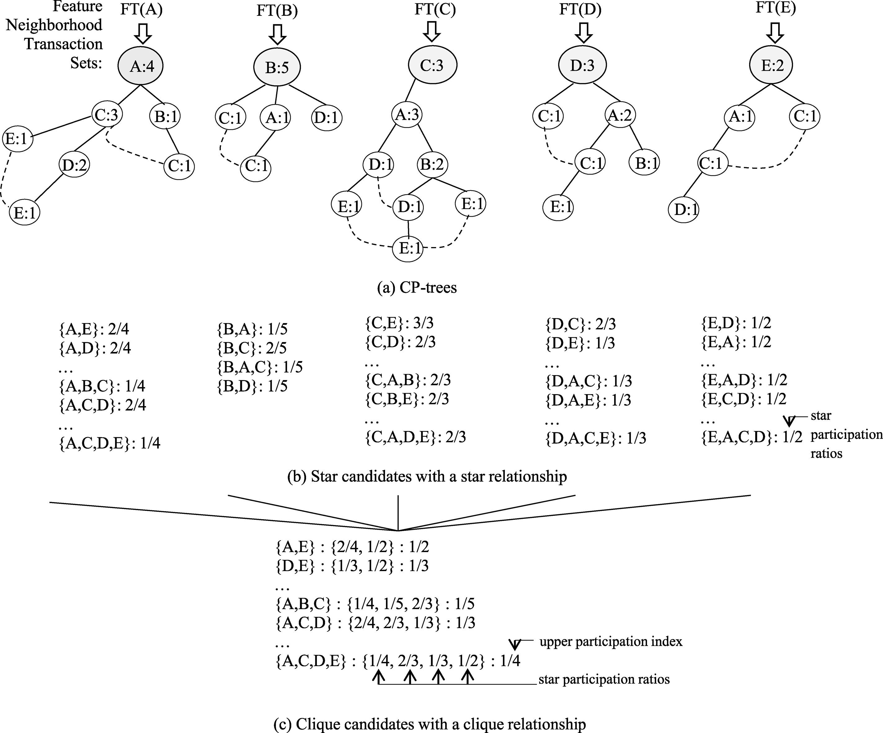

Next, we accumulate all possible subsets of features with following each branch path of the CP-tree (Line 6 in Algorithm 2). The feature type of the root node is added to each sub set as the first element of the set. The feature subsets generated are called to star candidates because the first item in a candidate set has neighbor relationships with all other items in the set. For example, in Fig. 5a, all star candidates generated from $D$ -CP-tree are {D, A}, {D, B}, {D, C}, {D, E}, {D, A, B}, {D, A, C}, {D, A, E} and {D, A, C, E}. The count information in the tree node gives the frequency of a feature set which has a star relation with the root node’s feature. For example, {D, A, C}’s frequency is 1 because the last element’s node count is 1.

.

Star participation ratio: Let $X$ be a set of features $X=\{f_{i},f_{1},\ldots,f_{i-1},f_{i+1},\ldots,f_{l}\}$ . The star participation ratio of feature $f_{i}$ in $X$ where $f_{i}$ is the first item, $\textit{StarPR}(X,f_{i})$ , is the fraction of $f_{i}$ -feature neighborhood transactions which include all items in the candidate $X$ , that is, $\frac{\textit{Number of }f_{i}-\textit{feature neighborhood transactions }\supseteq X}{\textit{Number of }f_{i}-\textit{feature % neighborhood transactions}}$ .

$\textit{StarPR}(X,f_{i})$ is computed with the count information in $f_{i}$ -CP-tree. Let $t$ be the count number of root node $f_{i}$ , and $s$ be the count of the node of the last feature of $X$ in the branch with all features in $X$ . $\textit{StarPR}(X,f_{i})$ is $\frac{s}{t}$ . For example, in the $D$ -CP-tree in Fig. 5c. The count of node E reached via nodes D, A and C is 1. That means, among three D feature objects, only one D object has neighbor relationships with all three A, C and E objects. Thus StarPR ({D, A, C, E}, D) $=$ $\frac{1}{3}$ . If $\textit{StarPR}(X,f_{i})$ is less than a given prevalence threshold $\theta$ , the feature set $X$ is not considered as a star candidate (Line 7–9 in Algorithm 2).

3.2.2 Generation of clique candidates

Co-location candidates (also called clique candidates) are generated with combining the star candidates survived from the star participation ratio-based pruning (Line 11 in Algorithm 2). For examples, a candidate {A, B, C} is generated with combining star candidates with three features A, B, and C, i.e., {A, B, C}, {B, A, C} and {C, A, B}.

.

Upper participation index: The $\textit{UpperPI}(X)$ of a candidate $X=\{f_{1},\ldots,f_{l}\}$ is defined as $\textit{UpperPI}(X)=\min_{f_{i}\in X}\{\textit{StarPR}(X,f_{i})\}$ .

We already know that each star participation ratio of a co-location candidate satisfies the prevalence threshold (line 11 in Algorithm 2). Thus the upper participation ratio index of the candidate is always greater than or equal to a given minimum prevalence threshold.

3.3 Candidate pruning

The co-location candidates generated can be presented using an enumeration tree. The co-location pattern search strategy is relevant to how the search space is traversed for the pattern discovery. This framework can adopt different search strategies. First, the general-to-specific search traverses the candidate space in a breadth-first manner and finds length $l-1$ co-locations before looking for length $l$ co-locations. Using the monotonicity property of participation index measure [14], if a candidate is determined as a non-prevalent set during the pattern discovery process, its all super sets are pruned out. This traversal method is used for finding closed co-locations and all prevalent co-located feature sets in this framework. Second, the specific-to-general search traverses in a depth-first manner, and looks for more specific prevalent co-located feature sets such as maximal co-locations. If a length $l$ candidate is a maximal co-location, we can prune out all subsets of length $l-1$ of the maximal.

3.4 Co-location instance search

To discover co-location patterns, we need to find the co-location instances of each candidate. This framework uses a filter-and-refine approach for efficiently finding the instance of co-locations.

.

A set of spatial objects, $I=\{o_{1},\ldots,o_{l}\}$ is a star instance of a feature set $X=\{f_{1},\ldots,f_{l}\}$ , if (1) $I$ contains an object of each feature in $X$ , and (2) the first object $o_{1}$ in $I$ has a neighbor relationship with each other object in $I$ , i.e., $R(o_{1},o_{j})=$ true for $2\leqslant j\leqslant l$ .

In the filter step, potential co-location instances of candidates (which are called star instances) are collected with scanning the neighborhood transaction records. To reduce the search space of star instances of candidates, we consider only “relevant” neighborhood transaction records. The star instances of a candidate $\{f_{1},f_{2},\ldots,f_{l}\}$ are collected from neighborhood records whose first item is the same with the first item $f_{1}$ in the candidate set, for example, $f_{1}$ -neighborhood transactions for a candidate $\{f_{1},f_{2},\ldots,f_{l}\}$ . For example, Fig. 6 shows the relevant neighborhood transactions based on the first element in candidates.

Figure 6.

Co-location instance search with relevant neighborhood transactions and subinstance lookups.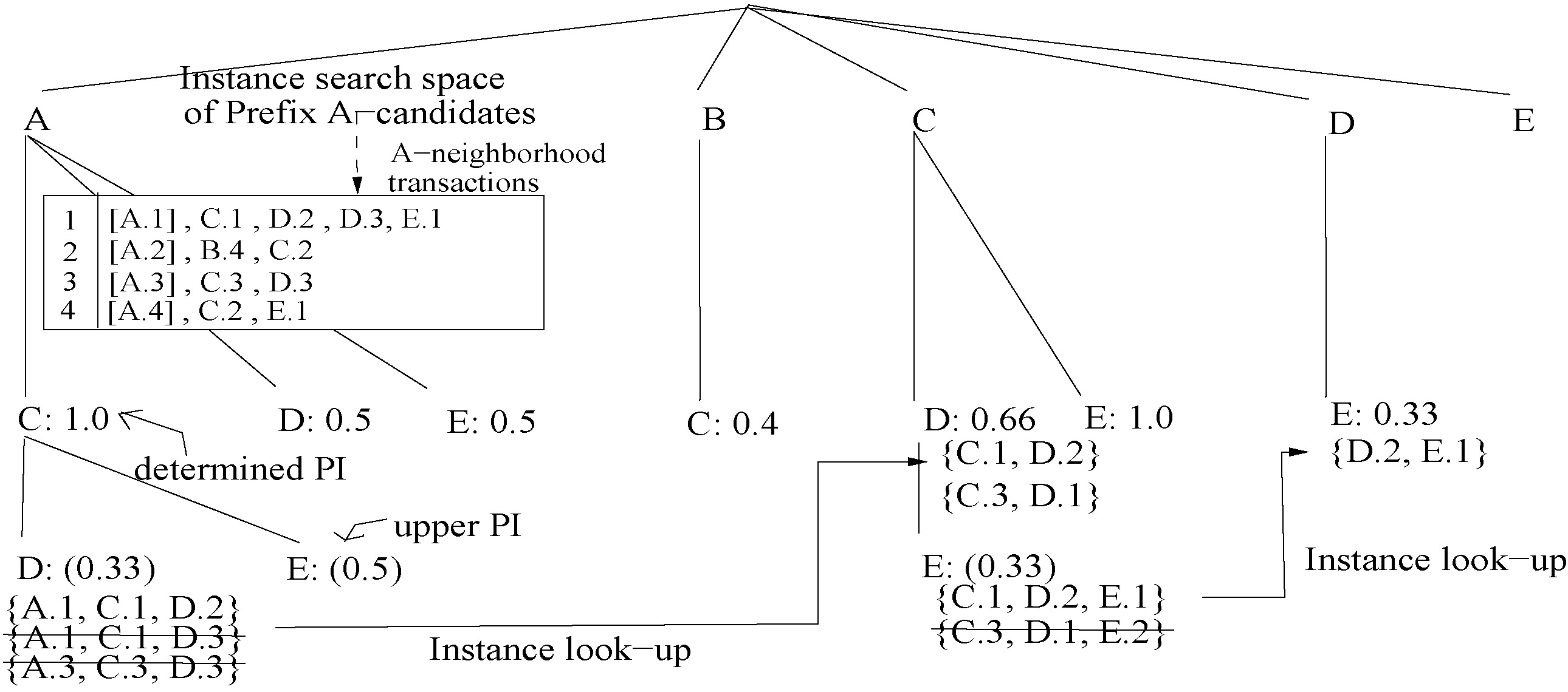

In the refine step, true co-location instances of a candidate can be filtered from its star instances. A star instance $\{o_{1},o_{2},\ldots,o_{l}\}$ is a co-location instance if all objects in its subset $\{o_{2},\ldots,o_{l}\}$ are neighbors each other because we know that $o_{1}$ has already neighbor relationships with each other objects $o_{2},\ldots,o_{l-1}$ and $o_{l}$ (Definition 7 and 10). The refine procedure depends on the traversal method of the candidate tree. If the candidate tree is traversed in a breadth-first manner, the instance-lookup scheme proposed in [40] is used for the refinement stage. The idea is to reuse length $l$ -l co-location instances for finding length $l$ co-location instances. A star instance $\{o_{1},o_{2},\ldots,o_{l}\}$ becomes a co-location instance of $\{f_{1},f_{2},\ldots,f_{l}\}$ , if $\{o_{2},\ldots,o_{l}\}$ is one of the co-location instances of $\{f_{2},\ldots,f_{l}\}$ .

3.5 Prevalence computation

The participation index value of a candidate is computed with its true co-location instances. If the prevalence value is greater than a given minimum threshold, the candidate becomes a prevalent co-located feature set.

4. Maximal and closed co-location mining

So far, we showed the main procedure of the algorithmic framework and how to find all prevalent co-location feature sets. Next, we present how maximal co-locations and closed co-locations are discovered in this framework. This section describes additional algorithmic strategies for mining maximal co-locations and closed co-locations in three parts: 1) candidate space browsing and pruning, 2) instance search, and 3) maximality or closeness check.

4.1 Maximal co-location mining algorithm

Algorithm 3 shows the pseudo codes of Maximal Co-location mining algorithm (MaxColoc).

Algorithm 3 MaxColoc algorithm
Input
$C$ : a set of clique candidates.
$N P$ : a set of all neighbor pairs.
$N T$ : a set of neighborhood transaction records.
Output
$R$ : a set of maximal co-location patterns
Variables
$\theta$ : a minimum prevalence threshold
$l$ : pattern length
$C_{l}$ : a set of length $l$ candidates
$MC_{l}$ : a set of length $l$ maximal candidate sets
tree: a subset tree for candidates
$c$ : a candidate set $<$ feature-set, pi, upperpi, ctl, instances, status $>$
$SI_{c}$ : a set of star instances of a candidate set $c$
$SI_{l}$ : a set of star instances of length $l$ feature sets $SI_{c}\in SI_{l}$
$CI_{c}$ : a set of true co-location instances of a candidate set $c$
Maximal co-location mining
1)–11) Neighborhood preprocess & candidate generation – Algorithms 1 and 2
12) $\textit{tree}=$ Build_candidate_tree ( $C$ );
13) $l=$ Max_length ( $C$ );
14) while ( $l\geqslant 2$ or $\textit{tree}\neq\emptyset$ ) do
15) $MC_{l}=$ Get_length_l_candidates (tree, $l$ );
16) $SI_{l}=$ Find_star_instances ( $MC_{l}$ , tree);
17) for each candidate $c\in MC_{l}$ do
18) $\textit{c.instances}=$ Find_clique_instances ( $SI_{l}$ , $c$ , $N P$ );
19) $c.pi=$ Calculate_pi (c.instances);
20) if $c.pi>\theta$ then Insert ( $c$ , $R_{l}$ );
21) end do
22) $R=R\cup R_{l}$ ;
23) $\textit{tree}=$ Subset_pruning_supersets ( $R_{l}$ , tree);
24) $l=l-1$ ;
25) end do
26) return $R$ ;

4.1.1 Candidate space browsing and pruning

MaxColoc traverses the enumeration tree of candidates in a hybrid manner, using both depth-first and breadth-first traversals as shown in Fig. 7. The depth-first traversal is used for quickly determining maximal co-located feature sets. We consider only maximal candidates.

Figure 7.

Candidate set pruning by a maximal set.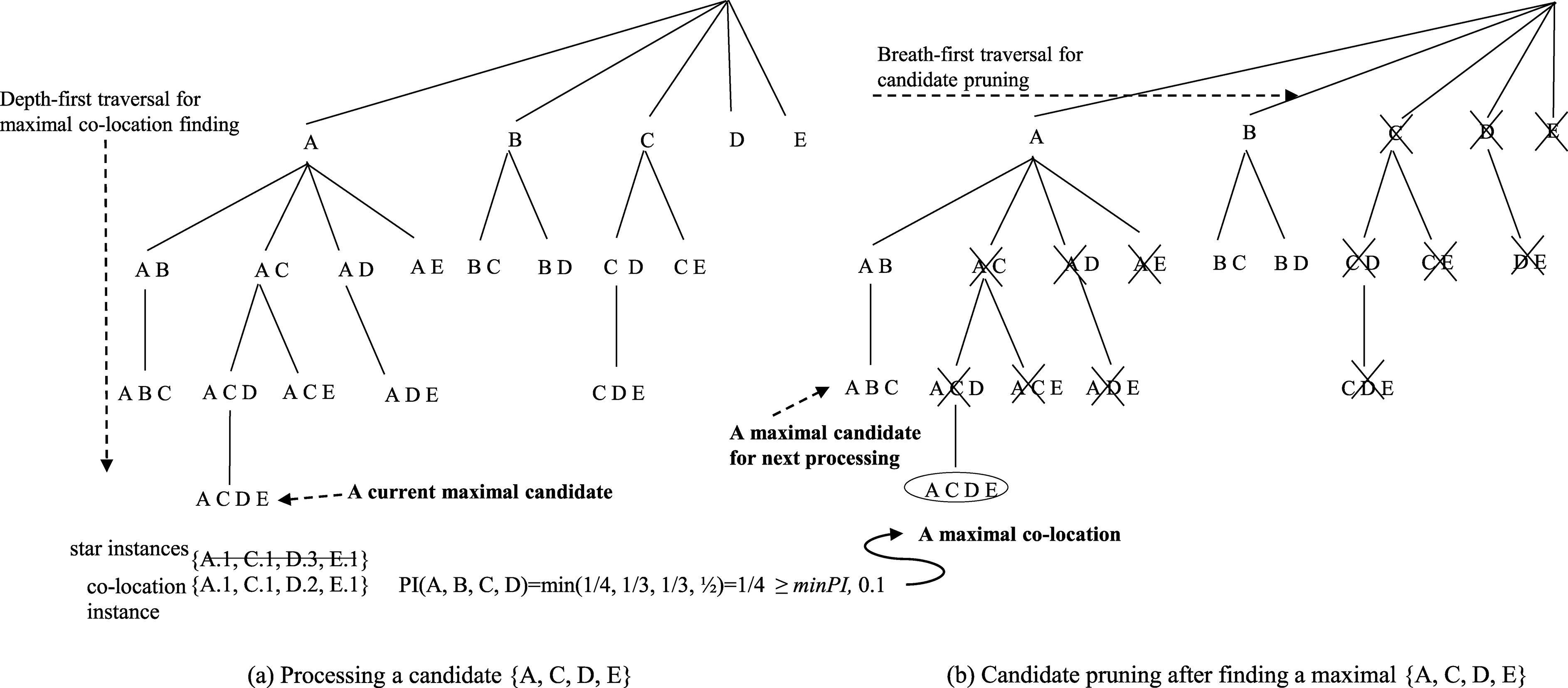

.

Maximal co-location candidate: A candidate set $X=\{f_{1},\ldots,f_{l}\}$ is a maximal co-location candidate if no super set of a co-location candidate $X$ is prevalent, i.e., for $X^{\prime}\supset X$ , $PI(X^{\prime})<\theta$ , where $\theta$ is a minimum prevalence threshold.

After uncovering maximal co-locations in the level, MaxColoc prunes out all sub candidate sets of the maximal co-location for further reducing candidate feature sets using the subset-pruning-by-supersets scheme (Line 23 in Algorithm 3). For the subset pruning, the candidate tree is navigated in the top-down and breadth-first manner. Let the feature set of a node in the candidate tree be termed the node’s head, and the possible extensions of the node be the tail. Let the head union tail of a node be HUT. The subsets of a maximal co-location are pruned out by determining whether or not the HUT of each node in the tree is a subset of the maximal co-location. If the HUT of a node is a subset of a maximal co-location, the subtree rooted at the node is pruned out. In the example of Fig. 7a, suppose that {A, C, D, E} is a maximal co-location. In the first level of the co-location candidate tree, the HUT of node A is {A, B, C, D, E} because its head is {A} and its tail is the set {B, C, D, E}. We cannot prune out the subtree of node A because its HUT is not a subset of {A, C, D, E}. However, the HUT of the node of C, {C, D, E}, is a subset of the maximal {A, C, D, E}. Thus, the subtree rooted at C is pruned out. Figure 7b shows the status of the subset tree after finding a maximal co-location {A, C, D, E}. This pruning scheme ensures we consider only maximal candidates for co-location instance search in the next step.

4.1.2 Instance search

For finding the instances of maximal co-location candidates, we follow the filter-and-refine idea. The star instances of candidates are first collected from their relevant neighborhood transactions (Line 16 in Algorithm 3). The refinement step filters out co-location instances from the star instances with the information of neighbor pair relations prepared in the preprocess stage (Line 18 in Algorithm 3).

4.1.3 Maximality check

MaxColoc finds prevalent co-located feature sets from only maximal candidates because non-maximal candidates are pruned out in the step of the subset-pruning-by-supersets. If a maximal candidate set is prevalent, it becomes a maximal co-location without any other check (Line 20 in Algorithm 3).

4.2 Closed co-location mining algorithm

Algorithm 4 shows the pseudo codes of Closed Co-location mining algorithm (ClosedColoc).

Algorithm 4 ClosedColoc algorithm
Input
$F=\{f_{1},\ldots,f_{m}\}$ : a set of spatial features.
$C$ : a set of clique candidates.
$N T$ : a set of neighborhood transaction records.
Output
$R$ : a set of closed co-located patterns
Variables
$\theta$ : a minimum prevalence threshold
$l$ : pattern length
tree: a subset tree for candidates
$C_{l}$ : a set of length $l$ candidates
$CC_{l}$ : a set of length $l$ closed candidates in a subset tree
$c$ : a candidate set $<$ feature-set, pi, upperpi, ctl, instances, status $>$
$SI_{l}$ : a set of candidate instances of length $l$ co-located feature-sets
Closed co-location mining
1)–11) Neighborhood preprocess & candidate generation – Algorithms 1 and 2
12) $P_{1}=F$ ;
13) $l=$ 2;
14) while $P_{l-1}\neq\emptyset$ do
15) $CC_{l}=$ Filter_Candidates ( $P_{l-1}$ , $C_{l}$ , $l$ , tree);
16) $SI_{l}=$ Find_star_instances ( $CC_{l}$ , tree);
17) for each candidate $c$ in $CC_{l}$ do
18) $\textit{c.instances}=$ Find_clique_instances ( $SI_{l}$ , $c$ , tree);
19) $c.pi=$ Calculate_pi (c.instances);
20) if $c.pi\geqslant\theta$ then
21) Insert ( $c$ , $P_{l}$ );
22) Insert_with_subsume_check ( $c$ , $R$ );
23) end if
24) end do
25) $l=l+1$ ;
26) end do
27) return $R$ ;

Algorithm 5 Generate_Candidates()
Generate_Candidates ( $P_{l-1}$ , $C_{l}$ , $l$ , tree);
1) while $CC_{l-1}\neq\emptyset$ do
2) $T=$ Generate_length_l_feature_sets ( $P_{l-1}$ );
3) for each event $c$ in $T$ do
4) for each length $l-1$ subset $s$ in $c$ do
5) if $s$ subset $\notin P_{l-1}$ then Remove ( $T$ , $c$ ); break;
6) end do
7) if $c\notin C_{l}$ then Remove ( $T$ , $c$ ); continue;
8) for all length $l-1$ subset $s$ in $c$ do
9) if $c$ ’s upperpi $<$ $s$ ’pi then $c$ .status $=$ ‘released’;
10) end do
11) $CS=$ Get_length2_subsets ( $c$ , $C_{2}$ );
12) for each subset $s$ in $C S$ do
13) end do
14) $\textit{c.ctl}=$ $\textit{c.ctl}\bigcap\textit{s.ctl}$ ;
15) Add_to_subsetTree ( $c$ , tree);
16) end do
17) end do
18) return $T$

Algorithm 6 Insert_with_subsume_check()
Insert_with_subsume_check ( $c$ , $R$ )
1) if $c$ .status $==$ ‘closed candidate’ then Insert ( $c$ , $R$ ); exit;
2) if $R$ ’s entry value $==$ $c$ .pi then
3) subsets $=$ Search_subsets ( $c$ );
4) if subsets $!=$ $\emptyset$ then
5) Remove (subsets, $R$ ); Insert ( $c$ , $R$ );
6) else Insert ( $c$ , $R$ );
7) else Insert ( $c$ , $R$ );

4.2.1 Candidate space browsing and pruning

ClosedCloc processes the candidate at each level of the candidate tree in a top-down and breadth-first manner. For further reducing candidates, ClosedColoc filters length $l$ candidates whose length $l-1$ sub feature sets are all prevalent, where $l\geqslant 2$ (Line 12 in Algorithms 4 and 5). Furthermore, we differentiate closed candidates from candidates. The closed candidate is defined as following:

.

Closed candidate: A candidate $X=\{f_{1},\ldots,f_{l}\}$ is a closed candidate if $X$ ’s UpperPI $<$ all PI values of its immediate (length $l-1$ ) prevalent sets.

4.2.2 Instance search

ClosedColoc finds co-location instances using the filter-and-refine method explained in the framework. In the filter step, the star instances of candidates are collected form their relevant neighborhood records (Line 16 in Algorithm 4). In the refinment step, ClosedColoc reuses co-location instance information from the previous level output. A star instance $\{o_{1},o_{2},\ldots,o_{l}\}$ of $\{f_{1},f_{2},\ldots,f_{l}\}$ becomes a clique instance if its sub instance $\{o_{2},\ldots,o_{l}\}$ is a co-location instance of $\{f_{2},\ldots,f_{l}\}$ as shown in Fig. 8a (Line 18 in Algorithm 4).

Figure 8.

Length 2 and Length-3 closed co-location mining.

4.2.3 Closedness check

If a candidate’s participation index satisfies a given prevalence threshold, the candidate is a prevalent co-located feature set (Line 21 in Algorithm 4). However we need to check whether the prevalent set is a closed set or not. We use two strategies for that. First, we use a hash-based subsumption check strategy (Line 22 in Algorithms 4 and 6). Let $X$ and $Y$ be two feature sets. We say that $X$ subsumes $Y$ , if and only if $Y\subset X$ and $PI(Y)=PI(X)$ . For quickly retrieving subsumed feature sets, potential closed co-location sets are stored in a hash data structure, and their PIs are used for the hash function. As shown in Fig. 8b we first retrieve an entry from the hash table with the hash key of PI of a prevalent co-located set $X$ , and next check if there is a feature set in the bucket which is a subset of $X$ . If there is a subsumed set, it is replaced with $X$ . The second strategy is, when we generate candidates, we examined whether the candidate is a closed candidate or not. Thus, if the prevalent co-located feature set was from a closed candidate, the set is included in the result set of possible closed co-locations without any further check.

5. Correctness and completeness

In this section, we prove the proposed algorithms are correct and complete in finding maximal and closed co-location patterns, respectively. We first give related lemmas.

.

Let $X=\{f_{1},\ldots,f_{l}\}$ be a set of spatial features. $PR(X,f_{i})\leqslant\textit{StarPR}(X,f_{i})$ where $1\leqslant i\leqslant l$ .

Proof: According to Definition 2, the participation ratio of feature $f_{i}$ in $X$ , $PR(X,f_{i})$ , is $\frac{\textit{Number of distinct objects of }f_{i}\textit{ in co-location instances of }X}{\textit{Number of objects of% }f_{i}}$ . According to Definition 8, the star participation ratio of feature $f_{i}$ in $X$ , $\textit{StarPR}(X,f_{i})$ , is $\frac{\textit{Number of }f_{i}-\textit{feature neighborhood transactions }\supseteq X}{\textit{Number of }f_{i}-\textit{feature % neighborhood transactions}}$ . Because one feature neighbor transaction is generated per each object, the number of $f_{i}$ -feature neighborhood transactions is the same with number of objects of $f_{i}$ . Let consider the case where $f_{i}$ is $f_{1}$ . The number of $f_{1}$ -feature neighborhood transactions which include all feature items in $X=\{f_{1},\ldots,f_{l}\}$ is the number of star instances of $X$ . Thus we can show that the number of objects of $f_{1}$ in co-location instances of $X$ is less than or equal to the number of star instances of $X$ . According to Definitions 10 and 1, the condition of a co-location of $X$ (i.e., $R(o_{i},o_{j})=$ true for $1\leqslant i<l$ , $i<j\leqslant l$ ) is more restrictive with including the condition of a star instance of $X$ (i.e., $R(o_{1},o_{j})=$ true for $2\leqslant j\leqslant l$ ). Thus the number of objects of $f_{1}$ in co-location instances of $X$ cannot be greater than the number of objects of $f_{1}$ in star instances of $X$ . Therefore, $PR(X,f_{1})\leqslant\textit{StarPR}(X,f_{1})$ . This can be generalized for all $f_{i}$ in $X$ where $1\leqslant i\leqslant l$ . Thus we conclude that $PR(X,f_{i})\leqslant\textit{StarPR}(X,f_{i})$ .

.

Let $X=\{f_{1},\ldots,f_{l}\}$ be a set of spatial features. $PI(X)\leqslant\textit{UpperPI}(X)\leqslant\textit{StarPR}(X,e_{i})$ , where $1\leqslant i\leqslant l$ .

Proof: According to Definition 2, $PI(X)=\min\{PR(X,f_{1}),\ldots,PR(X,f_{l})\}$ . According to Definition 9, $\textit{UpperPI}(X)=\min\{\textit{StarPR}(X,f_{1}),\ldots,\textit{StarPR}(X,f_% {l})\}$ . According to Lemma 1, $PR(X,f_{i})\leqslant\textit{StarPR}(X,f_{i})$ where $1\leqslant i\leqslant l$ . Therefore, $PI(X)\leqslant\textit{UpperPI}(X)\leqslant\textit{StarPR}(X,e_{i})$ , where $1\leqslant i\leqslant l$ .

.

Let $I=\{o_{1},\ldots,o_{l}\}$ be a star instance of a feature set $X=\{f_{1},\ldots,f_{l}\}$ . If the sub instance of $I$ excluding the first item $o_{1}$ , $\{o_{2},\ldots,o_{l}\}$ , is a co-location instance of $X=\{f_{2},\ldots,f_{l}\}$ , $I$ is a co-location instance of $X$ .

Proof: Please refer to [41].

.

The MaxColoc algorithm is complete and correct.

Proof: Completeness means that MaxColoc finds all maximal co-locations which satisfy Definition 5. Correctness means that all co-located feature sets, discovered by MaxColoc, are maximal co-locations. The completeness is explained by showing that the candidate generation and pruning procedure does not drop any potential maximal feature sets. The procedures to build CP-trees with feature neighborhood records, collect star candidates from each CP-tree, and generate co-location candidates with combining the star candidates are correct and do not miss any potential co-location candidates. According to Lemma 2, the StarPR based pruning does not remove any potential co-location candidates. Additional candidate pruning scheme, the subset-pruning-by-supersets, deletes only the subsets of maximal co-locations, since the comparison with the HUT of a node in the enumeration tree of candidates is correct, and the subsets of maximal co-locations cannot be maximal patterns by Definition 5. On the other hand, the correctness of the MaxColoc algorithm can be guaranteed by the co-location instance search method, prevalence check, and maximality check as well as the proof for the completeness. The filter step of instances is correct with gathering the potential instances (i.e., star instances) of candidates from their relevant neighborhood transactions according to Definitions 7 and 10. The refinement step to check the star instances with neighbor pair relations does not miss any true co-location instances. The value of the participation index of a candidate is computed with its true co-location instances. The participation index value is checked with the given prevalence threshold. By the subset-pruning-by-supersets scheme in MaxColoc, only maximal candidates are considered in the instance search and prevalence check. Therefore all prevalent candidate feature sets are maximal co-locations.

.

The ClosedColoc algorithm is complete and correct.

Proof: Completeness means that ClosedColoc finds all closed co-locations which satisfy Definition 4. Correctness means that the co-located feature sets discovered by ClosedColoc are closed co-locations. ClosedColoc uses the candidate generation procedure which is the same in the MaximalColoc. As shown in the proof of Theorem 1, the procedure does not miss any potential co-location candidates. Additional candidate pruning scheme in the CloseColoc is based on the property of anti-monotonicity of the participation index [14]. Because of participation index is monotonically non-increasing as the length of co-location increases, if a candidate is not prevalent, its super sets are pruned out. The subsumption check procedure removes only subsumed feature sets $Y$ by closed co-location $X$ such that $Y\subset X$ and $PI(Y)=PI(X)$ . The subsumed feature sets cannot be closed co-location by Definition 4. Therefore ClosedColoc finds a complete set of closed co-locations. On the other hand, the correctness of the ClosedColoc algorithm can be guaranteed by the co-location instance search method, prevalence check, and closeness check. The filter step of instances is correct because it gathers the potential instances (i.e., star instances) of candidates from their relevant neighborhood transactions by Definitions 7 and 10. Lemma 3 ensures the refinement procedure with the subinstance-lookup scheme does not miss any true co-location instance. The participation index value computed with true co-location instances is correct. The subsumption check is used to remove only non closed features in the result set. Thus, the final result set includes only closed co-locations.

6. Experiment result

This section presents the result of experimental evaluation of proposed MaxColoc and ClosedColoc algorithms.

6.1 Experimental setting

We used real data as well as synthetic data for this experiment. We generated synthetic data on a study area of 1,000 $\times$ 1,000 using a spatial point generator similar to a tool used in [41]. The synthetic dataset (DATA#1) has 20 event types and 14,639 data points. For real data, we used two data sources. A dataset (DATA#2) with 12,000 data points of 40 features was prepared from the points-of-interest (POI) data in California [31]. Category types such as church and school were used as feature types. The other real data is from the Environmental Protection Agency (EPA) databases [1]. This data contains information relative to environmental activities that affect air, water, and land within the United States. The forth dataset, DATA#3, includes the environmental facilities of Allen and Dekalb Counties in the state of Indiana extracted from the EPA database. The dataset has 663 data points of 17 features.

Figure 9.

Experimental procedure.

We compared MaxColoc and ClosedColoc with GeneralColoc+Maximal and GeneralColoc+Closed, which are based on a state-of-art co-location mining algorithm [29] but have a post-processing module for the final result pattern, maximal co-locations or closed co-locations. Figure 9 diagrams the experiment procedure. All the experiments were performed on a PC Linux system with 2.0 GB main memory.

Figure 10.

Comparisons of candidates.

6.2 Comparison of pattern candidates

To examine the effect of our candidate pruning schemes, we counted candidate feature sets considered for finding maximal co-locations and closed co-locations. In this experiment, the prevalence thresholds were 0.1 for DATA#1 and 0.1 for DATA#2. The prevalence threshold for DATA#3 was 0.4 because this dataset is a dense dataset. As shown in Fig. 10, the proposed approach generated significantly smaller number of candidates than the alternative methods in all the experimental settings. The comparison algorithm (GeneralColc) is one of co-location mining algorithms based on Apriori [12] which is a generation-and-test approach. It first finds prevalent length 2 ( $l=2$ ) co-location patterns, and then generates length $l+1$ candidates with frequent length $l$ co-located feature sets, searches their co-location instances and finds co-location patterns in a level-wise manner. The candidate generation is the same with apriori_gen in [2] for general frequent itemset mining. GeneralColc generates candidates with two main steps: candidate generation and pruning. After generating length $l+1$ candidates with joining length $l$ co-located feature sets, check whether their all subsets are frequent or not. If any subset of the candidate is not frequent, the candidate is pruned using the monotonic property of participation index. However, our candidate generation step generates candidates from data and filters using monotonic property of upper participation index (upperPI), and then further prunes candidates using additional schemes: subset-pruning-by-supersets for maximal co-locations and the monotonicity of participation index for closed co-locations.

In the result with DATA#2 (Fig. 10b), MaxColoc considered no length-2 candidates, because it processes long candidates in advance and prunes out all the subsets of discovered maximal co-locations. In contrast, MaxColoc+Maximal examined all possible pair feature sets. ClosedColoc also considered much fewer candidates compared to GeneralColoc+Closed. ClosedColoc started with small number of length-2 candidate sets which are generated in the preprocess stage. In contrast, the alternative method considers all possible length-2 feature sets. In Fig. 10f, the number of length 3 candidates of GeneralColoc+Closed was 40% less than ClosedColoc. This case happened when the number of length $l$ candidates survived from the upperPI based pruning in the preprocess was large even if some candidates in the candidate pool were pruned after finding length $l-1$ frequent patterns. When we see the length 4 case in the figure, both algorithms considered similar numbers of candidates because candidates generated using apriori_gen was similar with our candidates from the preprocess. When the difference of upperPI and PI values of candidates is large, ColosedColoc can consider more candidates than GeneralColoc+Closed. Although ColosedColoc shows overall better performance than the alternative method, to further reduce the candidates in ColosedColoc, we may consider a hybrid approach which chooses a smaller one among a set of candidates from preprocess and a set of candidates generated by apriori_gen at each level.

Figure 11.

Comparisons of performance.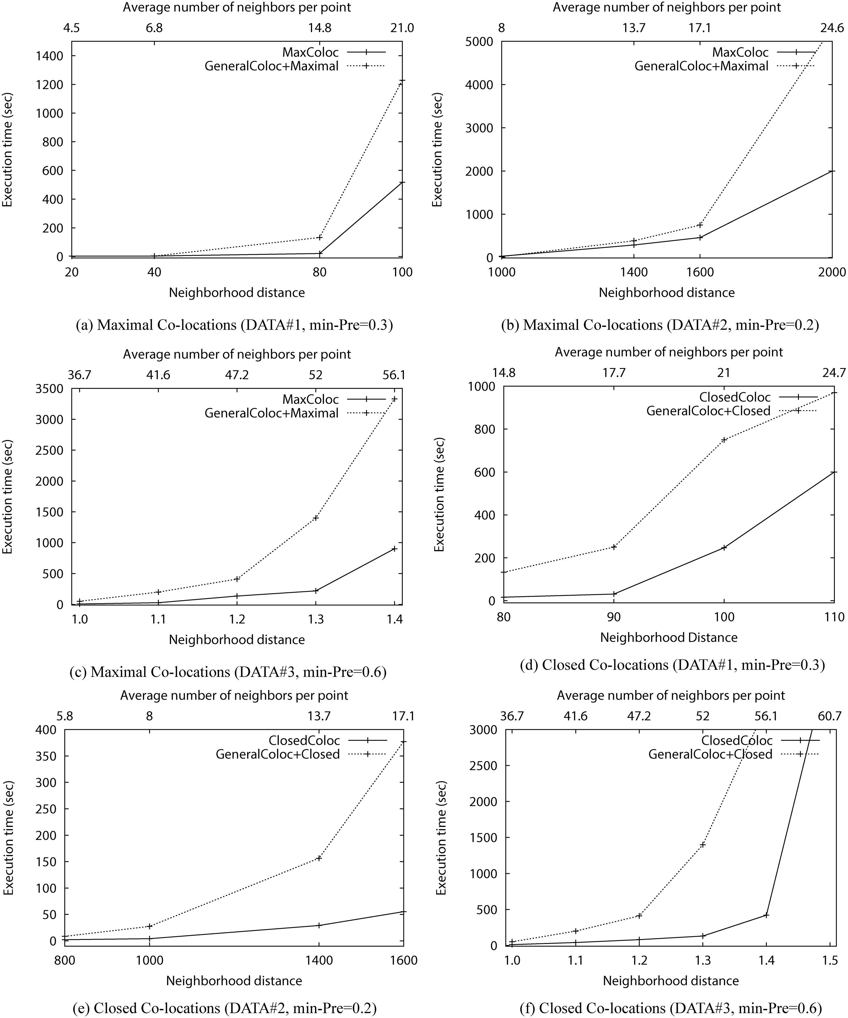

6.3 Performance evaluation

Next, we examined the effect of performance by neighborhood size. When the neighborhood size is larger, an object has a chance to have more neighbors. Figure 11 shows the results in finding maximal co-location and closed co-location patterns. X axis shows two values, neighbor distance threshold in the bottom X axis, and in the upper X axis, average number of neighbors per data object at each distance threshold. Different distance units were used on experiment datasets depending on the coordinate system of the real data or the data generator setting of the synthetic data. In the experiment with DATA#1, we used various distance thresholds from 20 to 110 units. When the distance was 20, the max number of neighboring objects of a data object was 17, and the average number of neighboring objects was 4.5. When the distance was 100, the max number of neighboring objects was 63, and the average number of neighbors per data object was 21. The prevalence threshold value was fixed to 0.3. In the experiment of DATA#2, we used 1,000, 1,400, 1,600 and 2,000 unites for the neighbor distance. When the distance was 2,000, the max number and average number of neighboring objects per data object were 184 and 24.6, respectively. In experiments with DATA#2, the prevalence threshold was 0.2, The difference between the running times of the two algorithms dramatically increased in larger distances, i.e., after distance 1600. In the last experiment with DATA#3, we increased the distance to a very small proportion, i.e., from 1.0 to. 1.5, because the EPA data is very dense. We also set a high prevalence threshold of 0.6. As shown in Fig. 11, MaxColoc always shows better performance than GeneralColoc+Maximal. In Fig. 11a, both MaxColoc and GeneralColoc+Maximal showed similar running times until distance value of 40. However, the difference of the running times dramatically increases after distance 80. Figure 11 also shows the results with ClosedColoc. The proposed algorithm also showed better performance than GeneralCloloc+Closed in the execution time.

7. Discussion

This section first describes the related works and then concludes this paper.

7.1 Related work

The problem of mining association rules, based on spatial relationships such as proximity and adjacency, is first discussed in Koperski and Han [17]. The work discovers subsets of spatial features frequently associated with a specific reference feature, e.g., the incidence of cancer. First, transaction records are created around instances of the reference feature. Then spatial association rules are derived using the apriori algorithm [2]. Morimoto [23] proposes a problem which finds frequent neighboring class sets using space partitioning and non-overlap grouping schemes for identifying neighboring objects. Since Shekhar and Huang [29] formalized spatial co-location mining problem, the problem has been popularly studied in spatial data mining literature [14, 39, 38, 41, 8, 23, 34, 37, 22, 33]. Huang et al. [14] define participation index which is statistically meaningful for co-location patterns and propose a spatial join-based co-location algorithm. Some studies indicates that the join-based method becomes inefficient with increasing data size because it requires massive amount of the pattern instance generation operations. Approaches to reduce expensive spatial join operations in co-location mining are proposed in the partial join method [39] and the join-less method [41]. The partial join approach [39] partitions the space with a set of neighborhood size grids disjointly, and keeps track of only neighbor relationships split across partitions using the spatial join operation. Xiao et al. [37] propose a density based approach which uses a clustering technique to find co-location patterns with a definition of density ratio to describe the neighbor relationship. Xiong et al. [38] study the co-location pattern mining problem for extended objects, such as lines and polygons. Zhang et al. [43] generalized the co-location mining problem to discover three types of patterns: star, clique, and generic patterns. Eick et al. [8] work on the problem of finding regional co-location patterns for sets of continuous variables in spatial datasets. Mohan et al. [22] propose a graph based approach to regional co-location pattern discovery. Qian et al. [25] find regional co-location patterns with $k$ -nearest neighbor graph. Wang et al. [33] study the problem of mining co-location rules from interval data. Flouvat et al. [10] propose a domain-driven co-location mining approach that combines constraint-based mining and cartographic visualization. Sengstock et al. [27] presents a new class of spatial interestingness measures of co-location pattern mining. Although Al-Naymat [4] worked for maximal co-location mining problems, there is no work to provide a common algorithmic framework for mining both maximal co-locations and closed co-locations as well as general co-location patterns.

7.2 Conclusion

Spatial co-location mining is a useful tool for uncovering implicit spatial relationship patterns in spatial data. However, identifying all prevalent co-located feature sets is computationally expensive, and many of result patterns have redundant information. This paper proposes the problem to discover compact sets of co-location patterns with maximal co-locations and closed co-locations. Our work focuses on developing an algorithmic framework to discover these reduced sets of co-location patterns as well as all prevalent co-locations. Two co-location algorithms, MaxColoc and ClosedColoc, are presented on the common framework. They use several schemes for reducing the number of candidate sets examined, efficiently searching co-location instances, and effectively determining the maximality or closedness of prevalent co-located feature sets. We proved that MaxColoc and ClosedColoc algorithms are correct and complete in finding maximal co-locations and closed co-locations, respectively. The empirical evaluation with real and synthetic datasets showed that the proposed framework is effective in generating the reduced sets of co-location patterns.

In the future, we plan to develop a unified framework for mining various co-location patterns in cloud computing environment. We expect that our algorithmic schemes such as the divide-and-conquer method for candidate generation and the filter-and-refine method for co-location instance search can be easily parallelized in a modern distributed computing platform such as Hadoop and Spark.

Footnotes

Acknowledgments

We thank Yeisol Woo for her support to help improve the presentation of this paper.

References

United States EPA (Environmental Protection Agency-FRS (Facility Registry System) Facilities. http://www.epa.gov/enviro/html/frs_demo/geospatial_data/geo_data_state_single.html.

Agarwal

and Srikant

, Fast algorithms for Mining association rules, in: Proc. of Int’l Conference on Very Large Databases (VLDB), 1994.

Akbari

Samadzadegan

and Weibel

, A generic regional spatio-temporal co-occurrence pattern mining model: A case study for air pollution, Journal of Geographical Systems 17(3) (2015), 249–274.

Al-Naymat

, Enumeration of Maximal Clique for Mining Spatial Co-location Patterns, in: Proc. of IEEE/ACS International Conference on Computer Systems and Applications, 2008.

Berg

Kreveld

Overmars

and Schwarzkopf

, Computational Geometry, Springer, 2000.

Dijkstra

Janssen

De Bakker

Bos

Lub

Van Wissen

L.J.G.

and Hak

, Using spatial analysis to predict health care use at the local level: A case study of type 2 diabetes medication use and its association with demographic change and socioeconomic status, PLoS ONE 8 (2013), e72730, 08.

Easter

Kriegel

and Sander

, Knowledge discovery in spatial databases, in: Proc. of International Conference on Artificial Intelligence, 1999.

Eick

C.F.

Parmar

Ding

Stepinski

T.F.

and Nicot

, Finding regional co-location patterns for sets of continuous variables in spatial datasets, in: Proc. of 16th Finding Regional Co-location Patterns for Sets of Continuous Variables in Spatial Datasets (ACM-GIS), 2008.

Flouvat

Selmaoui-Folcher

Gay

Rouet

and Grison

, Constrained colocation mining: Application to soil erosion characterization, in: Proceedings of the ACM Symposium on Applied Computing, 2010, pp. 1054–1059.

10.

Flouvat

Van Soc

J.-F.N.

Desmier

and Selmaoui-Folcher

, Domain-driven co-location mining, Geoinformatica 19(1) (2015), 147–183.

11.

Miller

H.J.

and Han

, Geographic Data Mining and Knowledge Discovery, Taylor and Francis, 2001.

12.

Han

Kamber

and Pei

, Data Mining: Concepts and Techniques, Second Edition, Morgan Kaufmann, 2005.

13.

Han

Pei

and Yin

, Mining Frequent Patterns Without Candidate Generation, in: Proc. of the ACM SIGMOD Conference on Management of Data, 2000.

14.

Huang

Shekhar

and Xiong

, Discovering colocation patterns from spatial data sets: A general approach, IEEE Transactions on Knowledge and Data Engineering 16(12) (2004), 1472–1485.

15.

Patel

D.J.D.J.M.

, Partition Based Spatial-Merge Join, in: Proc. of the ACM SIGMOD Conference on Management of Data, Montreal, Canada, June 1996, pp. 259–270.

16.

Jung

and Sun

, Development of a giservice based on spatial data mining for location choice of convenience stores in taipei city, Geoinformatics 2016: Spatial Information Technology, 2006, p. 6421.

17.

Koperski

and Han

, Discovery of Spatial Association Rules in Geographic Information Databases, in: Proc. of International Symposium on Large Spatial Data Bases, Maine, 1995, pp. 47–66.

18.

Lee

and Phillips

, Urban crime analysis through areal categorized multivariate association mining, Applied Artificial Intelligence 22(5) (2008), 483–499.

19.

Leibovici

Claramunt

Guyader

D.L.

and Brosset

, Local and global spatio-temporal entropy indices based on distance-ratios and co-occurrences distributions, Journal of Geographical Information Science 28(5) (2014), 1061–1084.

20.

Adilmagambetov

Mohomed Jabbar

M.S.

ZaÃ¯ane

O.R.

Osornio-Vargas

and Wine

, On discovering co-location patterns in datasets: A case study of pollutants and child cancers, Geoinformatica 20(4) (2016), 651–692.

21.

Mennis

and Liu

J.W.

, Mining association rules in spatio-temporal data: An analysis of urban socioeconomic and land cover change, Transactions in GIS 9(1) (2005), 5–17.

22.

Mohan

Shekhar

Shine

ROgers

Jiang

and Wayant

, A Neighborhood Graph based Approach to Regional Co-location Pattern Discovery: A Summary of Results, in: Proc. of the ACM SIGSPATIAL International Conference on Advances in Geographic Information Systems (ACM SIGSPATIAL GIS), 2011.

23.

Morimoto

, Mining Frequent Neighboring Class Sets in Spatial Databases, in: Proc. ACM SIGKDD Int’l Conference on Knowledge Discovery and Data Mining, 2001.

24.

Phillips

and Lee

, Mining top-k and bottom-k correlative crime patterns through graph representations, in: Proceedings of the IEEE International Conference on Intelligence and Security Informatics, 2009, pp. 25–30.

25.

Qian

Chiew

and Huang

, Mining regional co-location patterns with knns, Journal of Intelligent Information Systems 42(3) (2014), 485–505.

26.

Roddick

and Spiliopoulou

, A Bibliography of Temporal, Spatial and Spatio-Temporal Data Mining Research, In Proc. SIGKDD Explorations 1(1) (1999): 34–38.

27.

Sengstock

Gertz

and Canh

T.V.

, Spatial interestingness measures for co-location pattern mining, in: Proceedings of IEEE International Conference on Data Mining Workshop, 2012, pp. 821–826.

28.

Shekhar

and Chawla

, Spatial Databases: A Tour, Prentice Hall, ISBN 0130174807, 2003.

29.

Shekhar

and Huang

, Co-location Rules Mining: A Summary of Results, in: Proc. of Int’l Symposium on Spatio and Temporal Database (SSTD), 2001.

30.

Sierra

and Stephens

C.R.

, Exploratory analysis of the interrelations between co-located boolean spatial features using network graphs, Journal of Geographical Information Science 26(3) (2012), 441–468.

31.

Survey

U.G.

, http://www.usgs.gov/.

32.

Tobler

, A computer movie simulating urban growth in the detroit region, Economic Geography 46(2) (1970), 234–240.

33.

Wang

Chen

Zhao

and Zhou

, Efficiently mining co-location rules on interval data, in: Proceedings of International Conference on Advanced Data Mining and Applications: Part I, 2010, pp. 477–488.

34.

Ding

Jiamthapthaksin1

Parmar

Jiang

Stepinski

T.F.

and Eick

C.F.

, Towards Region Discovery in Spatial Datasets, in: Proc. of International Pacific-Asia Conference on Knowledge Discovery and Data Mining (PAKDD), 2008.

35.

Weiler

Schmid

K.A.

Mamoulis

and Renz

, Geo-social co-location mining, in: Proc. of International ACM Workshop on Managing and Mining Enriched Geo-Spatial Data, 2015, pp. 19–24.

36.

wen Hsiao

shu Tsai

and chiang Wang

, Spatial data mining of colocation patterns for decision support in agriculture, Asian Journal of Health and Information Sciences 1(1) (2006), 61–72.

37.

Xiao

Xie

Luo

and Ma

, Density based co-location pattern discovery, in: Proc. of 16th Finding Regional Co-location Patterns for Sets of Continuous Variables in Spatial Datasets (ACM-GIS), 2008.

38.

Xiong

Shekhar

Huang

Kumar

and Yoo

J.S.

. A Framework for Discovering Co-location Patterns in Data Sets with Extended Spatial Objects, in: Proc. of SIAM International Conference on Data Mining (SDM), 2004.

39.

Yoo

J.S.

and Shekhar

, A Partial Join Approach for Mining Co-location Patterns, in: Proc. of ACM International Symposium on Advances in Geographic Information Systems (ACM-GIS), 2004.

40.

Yoo

J.S.

and Shekhar

, A Join-less Apporach for Spatial Co-location Mining: A Summary of Results, in: Proc. of IEEE International Conference on Data Mining (ICDM), 2005.

41.

Yoo

J.S.

and Shekhar

, A join-less approach for mining spatial co-location patterns, IEEE Transactions on Knowledge and Data Engineering 18(10) (2006).

42.

, Spatialco-location pattern mining for location-based services in roadnetworks, Expert Systems With Applications 46 (2016), 324–335.

43.

Zhang

Mamoulis

Cheung

and Shou

, Fast Mining of Spatial Collocations, in: Proc. of ACM SIGKDD International Conference on Knowledge Discovery and Data Mining, 2004.