Canal-LASSO: A sparse noise-resilient online linear regression model

Abstract

Least absolute shrinkage and selection operator (LASSO) is one of the most commonly used methods for shrinkage estimation and variable selection. Robust variable selection methods via penalized regression, such as least absolute deviation LASSO (LAD-LASSO), etc., have gained growing attention in works of literature. However those penalized regression procedures are still sensitive to noisy data. Furthermore, “concept drift” makes learning from streaming data fundamentally different from the traditional batch learning. Focusing on the shrinkage estimation and variable selection tasks on noisy streaming data, this paper presents a noise-resilient online learning regression model, i.e. canal-LASSO. Comparing with the LASSO and LAD-LASSO, canal-LASSO is resistant to noisy data in both explanatory variables and response variables. Extensive simulation studies demonstrate satisfactory sparseness and noise-resilient performances of canal-LASSO.

Keywords

LASSO variable selection noise-resilient streaming data online learning

1. Introduction

Selecting significant explanatory variables is one of the most vital issues in statistical analysis and data mining [1]. Penalized regression methods consisting of loss function and penalized term (also known as regularization term) are widely used to select variables, such as LASSO [2], SCAD [3], and adaptive LASSO [4], etc. However, most of those methods are closely related to the least squares method. As far as we know that the ordinary least squares (OLS) method is sensitive to outliers in the scenario of finite samples, and consequently, the outliers may cause serious problems for the least squares based methods for variable selection. It is desirable to replace the least squares criterion with a noise-resilient one. To construct a robust objective function for regression, Fan and Li proposed a general framework of penalized objective function, i.e. to minimize following objective function with respect to $\boldsymbol{\beta}$ [3].

$\displaystyle L=\sum^{n}_{i=1}\ell(y_{i}-\boldsymbol{x}^{T}_{i}\boldsymbol{% \beta})+n\sum^{d}_{j=1}{p_{\lambda_{nj}}(|{\beta}_{j}|)},$ (1)

where $\ell(\cdot)$ is the Huber’s function. Since then, various noise-resistant loss functions $\ell(\cdot)$ and regularization terms $p_{\lambda_{nj}}(|{\beta}_{j}|)$ have been proposed and studied widely. Among them, based on the least absolute deviation (LAD) criterion [5], Wang et al. proposed the LAD-LASSO where $\ell(z)=|z|$ and $p_{\lambda_{nj}}(|{\beta}_{j}|)=\lambda_{nj}|{\beta}_{dj}|$ [6]. This procedure was proved to be able to reduce the impact of outliers to a certain extent. However, the impact of outliers is not eliminated completely. A loss function with a superior robustness performance is very fascinating and in urgent need. As discussed above, the motivation aims to study a noise-resilient procedure for variable selection, which inspires us to introduce a more robust loss function.

Besides, due to the rapid development of the Internet and the Internet of things, an ever increasing amount of data is available in streaming fashion [7]. It has been a critical problem to learn the prediction model from streaming data [8, 9]. Moreover, the statistical properties of the target variable, i.e. $p(y|\boldsymbol{x})$ , which the model is trying to predict, may vary over time. It would reduce the accuracy of the prediction model as time goes by [10]. Thus, learning from streaming data has become increasingly critical [11, 12, 13] in the community of machine learning and data mining.

To tackle the above issues, in this paper, we have proposed a new noise-resilient online linear regression method that is robust to outliers for streaming data. Specifically, we introduce a noise-resilient loss function named as canal loss $\ell^{\delta}_{\epsilon}$ to resist the negative impact of the noisy data and further put forward the canal-LASSO method for noise-resilient variable selection. Employing the online gradient descent (OGD) algorithm, we optimize the objective function (canal-LASSO) in the online setting. Furthermore, to reduce the impact of noisy data effectively, an adjusting strategy is given to dynamically tune the threshold parameters $\epsilon$ and $\delta$ of canal loss in the proposed algorithm. Assuming large-scale examples arrive consecutively one by one, in the online learning process, the regression coefficients $\boldsymbol{\beta}$ and regularization parameters $\boldsymbol{\lambda}$ are updated iteratively with sequential incorporated examples. The noise-resilient online canal-LASSO we proposed in this paper has three major merits:

Model sparsity: as can be seen from Fig. 2, only a fraction of examples (with the residual error in ( $-\epsilon-\delta,-\epsilon$ ) and ( $\epsilon,\epsilon+\delta$ )) will be used to adjust regression coefficients. It is designed to reduce the computational cost and enjoy the perfect scalability property.

Noise-resilient: by tuning threshold parameter $\delta$ dynamically, the noisy data which would lead to large absolute error (larger than the threshold parameter $\epsilon+\delta$ ) will be identified and not be used to adjust regression coefficients.

Real-time: the proposed canal-LASSO tunes the regularization parameters $\boldsymbol{\lambda}$ and updates the regression coefficients $\boldsymbol{\beta}$ for regularized linear model dynamically in real time.

The remainder of this paper is organized as follows. In Section 2, we review the related work along LASSO-type procedures and then introduce the noise-resilient online learning algorithm for linear regression. In Section 3, we conduct numerical simulations and experiment on benchmark datasets to compare the performance of the proposed canal-LASSO with LASSO and LAD-LASSO. Finally, Section 4 concludes the paper with a short discussion.

2. Related works

In this section, we review the related work from two aspects: robust regression estimators and online learning.

variable selection has a rich history in statistics. Various insights of variable selection were proposed (Non-negative Garrote, Bridge regression) before Tibshirani introduced the celebrated LASSO estimator [14, 15, 2]. Due to the lack of desired statistical properties, different penalties that satisfy some criteria such as sparsity, persistency, etc. were introduced in the past decades, like SCAD [3], MCP [16] and Adaptive LASSO [4]. On the other hand, the variable selection methods with structured penalties (e.g. features are dependent and/or there exists group structures between features) have become more popular because of the ever-increasing need to deal with complicated data, such as Elastic Net [17], Group LASSO [18], and so forth. The robust variable selection is a new topic by incorporating the robust losses in robust statistics area into the model, which performs well under noisy scenarios empirically [19, 20, 21]. For instance, LAD-LASSO is a typical example of consistent variable selection method that is noise-resilient [6].

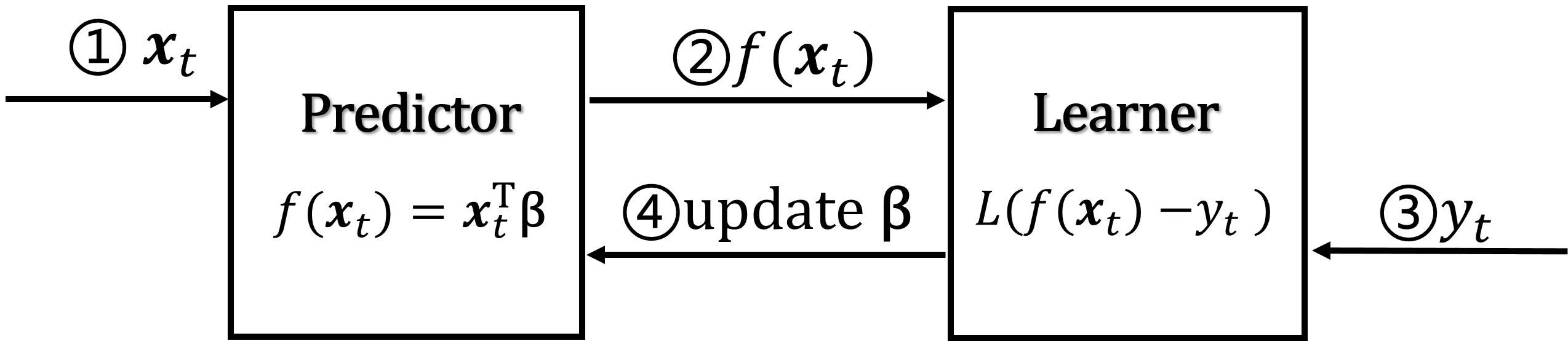
In the past decades, a great deal of research has been performed on inductive learning methods such as LASSO [2], artificial neural networks [22, 23], and support vector regression [24], etc. All of these techniques have been successfully applied to a lot of real-world problems. However, their standard application requires the availability of all of the training data at the same time [25], which makes them problematic in large-scale data mining applications and streaming data mining tasks [26, 27]. Comparing with the traditional batch learning framework, online learning algorithm (shown in Fig. 1) is another learning framework for samples learning in the streaming fashion so that it enjoys good properties of scalability and real-time. In recent years, great attentions have been paid to develop online learning methods in the machine learning community, such as online ridge regression [28, 29], adaptive regularization for LASSO [30], Projectron [31] and bounded online gradient descent algorithm [32], etc.

Figure 1.

An illustration schematic of the online regression learning procedure.

3. Method

Most of the existing online regression algorithms are primarily designed to learn information from clean data [30, 33]. However, due to the imperfect human labeling process and the sensor fault, noisy data is inevitable and ruinous. In this section, we have proposed a noise-resilient online learning algorithm for linear regression on streaming data. Motivated by the ramp loss designed for classification problem [34], we have proposed a noise-resilient loss function, named canal loss, for regression based on the well-known $\epsilon$ -insensitive loss [24]. Furthermore, we have exploited a novel strategy to adjust the canal loss parameters $\epsilon$ and $\delta$ dynamically.

3.1 Canal-LASSO

Consider the linear regression model

$\displaystyle y_{i}=\boldsymbol{x}_{i}^{T}\boldsymbol{\beta}+\varepsilon_{i},i% =1,2,\ldots,n,$ (2)

where $\boldsymbol{x}_{i}=[x_{1i},x_{2i},\ldots,x_{di}]^{T}\in\mathbb{R}^{d}$ is d-dimensional explanatory variable, $\boldsymbol{\beta}=[\beta_{1},\beta_{2},\ldots,\beta_{d}]^{T}\in\mathbb{R}^{d}$ are the associated regression coefficients, $\epsilon_{i}$ are iid random errors with mean of 0. Usually, regression coefficients of Eq. (2) can be estimated by minimizing the ordinary least squares (OLS) criterion. Meanwhile, to shrink insignificant coefficients to 0, Tibshirani proposed the primary LASSO criterion [2]:

$\displaystyle{\rm LASSO}^{1}:L(\boldsymbol{\beta})=\sum^{n}_{i=1}(y_{i}-% \boldsymbol{x}^{T}_{i}\boldsymbol{\beta})^{2}+n\lambda\sum^{d}_{j=1}|\beta_{j}|,$ (3)

where $\lambda>0$ is a fixed tuning parameter. Since all regression coefficients are penalized by the same regularization parameter $\lambda$ , the resulting estimators of $\boldsymbol{\beta}$ may suffer an apparent bias. To deal with this issue, Zou developed the following adaptive LASSO criterion [4]:

$\displaystyle{\rm LASSO}^{2}:L(\boldsymbol{\lambda},\boldsymbol{\beta})=\sum^{% n}_{i=1}(y_{i}-\boldsymbol{x}^{T}_{i}\boldsymbol{\beta})^{2}+n\sum^{d}_{j=1}% \lambda_{j}|\beta_{j}|,$ (4)

which allows for different tuning parameters $\lambda_{j}$ corresponding to different coefficients $\beta_{j}$ . As a result, the modified ${\rm LASSO}^{2}$ is able to produce sparse solutions more effectively than ordinary ${\rm LASSO}^{1}$ . Since the OLS criterion used in ${\rm LASSO}^{1}$ and ${\rm LASSO}^{2}$ is more sensitive to outliers than the LAD criterion [5], Wang et al. further modified the ${\rm LASSO}^{2}$ as following [6]:

$\displaystyle{\rm LAD-LASSO}:L(\boldsymbol{\lambda},\boldsymbol{\beta})=\sum^{% n}_{i=1}|y_{i}-\boldsymbol{x}^{T}_{i}\boldsymbol{\beta}|+n\sum^{d}_{j=1}% \lambda_{j}|\beta_{j}|.$ (5)

As can be seen, the LAD-LASSO combines the LAD criterion and the $\ell_{l}$ regularization, hence the resulting estimator is expected to be more robust than LASSO and also enjoys the property of sparse representation. After replacing the OLS criterion with the LAD criterion, the LAD-LASSO become more robust than ${\rm LASSO}^{2}$ . Unfortunately, LAD-LASSO can not eliminate the negative influence of noise data completely.

To obtain a noise-resilient LASSO-type estimator, we propose the following canal loss by modifying the classical $\epsilon$ -insensitive loss function $\ell_{\epsilon}(z)=\max\{0,|z|-\epsilon\}$ with a noise-resilient parameter $\delta$ :

$\displaystyle\ell_{\epsilon}^{\delta}(z_{i})=\text{min}\{\delta,\text{max}\{0,% |z_{i}|-\epsilon\}\}$ (6)

where $z_{i}=y_{i}-\boldsymbol{x}^{T}_{i}\boldsymbol{\beta}$ , $\epsilon>0$ and $\delta>0$ are the threshold tuning parameters.

Figure 2.

I. Absolute loss; II. $\epsilon$ -insensitive loss; III. Canal loss.

The illustration of three loss functions is shown in Fig. 2. Both the absolute loss function and the $\epsilon$ -insensitive loss function are sensitive to outliers. The upper bound of the proposed canal loss function is fixed as a constant, i.e. $\delta$ , which would significantly reduce the negative impact of outliers and make it a noise-resilient loss function. Taking advantage of canal loss, we have modified the LAD-LASSO and proposed the following canal-LASSO:

$\displaystyle{\rm canal-LASSO}:L=\sum^{n}_{i=1}\ell_{\epsilon}^{\delta}(z_{i})% +n\sum^{p}_{j=1}\lambda_{j}|\beta_{j}|.$ (7)

It is obvious that canal loss approximates to the absolute loss under the process of $\epsilon\to 0$ and $\delta\to+\infty$ , which is shown more clearly in the following equation:

$\displaystyle\lim_{\epsilon\to 0,\delta\to+\infty}\ell_{\epsilon}^{\delta}(z_{% i})=\lim_{\epsilon\to 0,\delta\to+\infty}\min\{\delta,\text{max}\{0,|z_{i}|-% \epsilon\}\}=|z_{i}|.$ (8)

It is expected that the proposed canal-LASSO is robust against outliers and also enjoys the property of sparse representation.

3.2 Online learning algorithm for canal-LASSO

In order to solve the canal-LASSO model effectively, we have employed the online gradient descent (OGD) algorithm proposed our optimization strategy by minimizing

$\displaystyle L(\boldsymbol{\lambda},\boldsymbol{\beta})=\sum^{n}_{t=1}\ell_{% \epsilon}^{\delta}(z_{t})+n\sum^{d}_{j=1}\lambda_{j}|{\beta}_{j}|,$ (9)

where $z_{t}=\boldsymbol{x}^{T}_{t}\boldsymbol{\beta}-y_{t}$ .

Firstly, many methods have been put forward to determine the regularization parameter $\boldsymbol{\lambda}$ in literatures, such as cross-validation, AIC, BIC, etc. In order to facilitate the computation and ensure the consistent variable selection, we have optimized the regularization parameter by minimizing a BIC-type objective function [6], i.e.,

$\displaystyle\min_{\boldsymbol{\lambda}}\sum^{n}_{t=1}\ell_{\epsilon}^{\delta}% (z_{t})+n\sum^{d}_{j=1}\lambda_{j}|\beta_{j}|-\log(0.5n\lambda_{j})\log(n).$ (10)

This leads to $\lambda_{j}=\frac{\log(n)}{n|{\beta}_{j}|}$ , i.e., $\boldsymbol{\lambda}=\left[\frac{\log(n)}{n|{\beta}_{1}|},\frac{\log(n)}{n|{% \beta}_{2}|},\ldots,\frac{\log(n)}{n|{\beta}_{d}|}\right]$ . Note that the update of $\boldsymbol{\lambda}$ is dependent on the estimation of $\boldsymbol{\beta}$ .

Secondly, Eq. (9) is not a convex optimization problem but it can be reformulated as a difference of convex (DC) programming. The Concave-Convex Procedure (CCCP) may be applied to solve this problem. However, CCCP belongs to the category of batch learning algorithms and does not satisfy the real-time requirement when dealing with streaming data. To find a near-optimal solution, in this work, we have employed the well-known OGD framework. It is a trade-off between the accuracy and scalability. In order to minimize Eq. (9) by OGD, we reformulate it to be

$\displaystyle\arg\min_{\boldsymbol{\beta}}L(\boldsymbol{\beta})\Leftrightarrow% \arg\min_{\boldsymbol{\beta}}\sum^{n}_{t=1}{[\underbrace{\ell_{\epsilon}^{% \delta}(z_{t})+\sum^{d}_{j=1}\lambda_{j}|\beta_{j}|}_{\mathcal{J}_{t}(% \boldsymbol{\beta})}]},$ (11)

and then we solve the optimization problem under the basic framework of OGD algorithm,

$\displaystyle\boldsymbol{\beta}^{(t)}=\boldsymbol{\beta}^{(t-1)}-\eta_{t}% \nabla_{\boldsymbol{\beta}}{\mathcal{J}_{t}(\boldsymbol{\beta})}|_{\boldsymbol% {\beta}=\boldsymbol{\beta}^{(t-1)}}.$ (12)

Here, $\eta_{t}$ is the t-th stepsize satisfying the following constraints $\sum^{n}_{t=1}\eta^{2}_{t}<\infty$ and $\sum^{n}_{t=1}\eta_{t}=\infty$ when $n\to\infty$ [35]. Instead of computing the full gradient of $L(\boldsymbol{\lambda},\boldsymbol{\beta})$ exactly, the notation $\nabla_{\boldsymbol{\beta}}{\mathcal{J}_{t}(\boldsymbol{\beta})}|_{\boldsymbol% {\beta}=\boldsymbol{\beta}^{(t-1)}}$ stands for the derivative of ${\mathcal{J}_{t}(\boldsymbol{\beta})}$ with regard to $\boldsymbol{\beta}=\boldsymbol{\beta}^{(t-1)}$ . We can deduce $\nabla_{\boldsymbol{\beta}}{\mathcal{J}_{t}(\boldsymbol{\beta})}|_{\boldsymbol% {\beta}^{(t)}=\boldsymbol{\beta}^{(t-1)}}$ as following

$\displaystyle\nabla_{\boldsymbol{\beta}}{\mathcal{J}_{t}(\boldsymbol{\beta})}|% _{\boldsymbol{\beta}=\boldsymbol{\beta}^{(t-1)}}=\left\{\begin{array}[]{ll}-% \boldsymbol{x}_{t}+\boldsymbol{\lambda}^{(t-1)}{\rm sign}(\boldsymbol{\beta}^{% (t-1)}),&\text{if }-\epsilon-\delta\leqslant z_{t}<-\epsilon,\\ \boldsymbol{x}_{t}+\boldsymbol{\lambda}^{(t-1)}{\rm sign}(\boldsymbol{\beta}^{% (t-1)}),&\text{if }\epsilon\leqslant z_{t}<\epsilon+\delta,\\ \boldsymbol{\lambda}^{(t-1)}{\rm sign}(\boldsymbol{\beta}^{(t-1)}),&\text{% otherwise},\\ \end{array}\right.$ (13)

where $z_{t}=\boldsymbol{x}^{T}_{t}\boldsymbol{\beta}^{(t-1)}-y_{t}$ . Substituting the gradient Eq. (13) into Eq. (12),

$\displaystyle\boldsymbol{\beta}^{(t)}=\left\{\begin{array}[]{ll}\boldsymbol{% \beta}^{(t-1)}-\eta_{t}(\boldsymbol{x}_{t}{\rm sign}(z_{t})+\boldsymbol{% \lambda}^{(t-1)}{\rm sign}(\boldsymbol{\beta}^{(t-1)})),&\text{if }\epsilon% \leqslant|z_{t}|<\epsilon+\delta,\\ \boldsymbol{\beta}^{(t-1)}-\eta_{t}(\boldsymbol{\lambda}^{(t-1)}{\rm sign}(% \boldsymbol{\beta}^{(t-1)})),&\text{otherwise}.\\ \end{array}\right.$ (14)

Note that the update of $\boldsymbol{\beta}$ is dependent on $\boldsymbol{\lambda}$ .

Finally, as shown in Eq. (14), there are a sparse parameter $\epsilon\geqslant 0$ and a noise-resilient parameter $\delta\geqslant 0$ in the proposed canal-LASSO. If the parameter $\epsilon$ approximates 0 and $\delta$ gets closer to $+\infty$ , the proposed method is equivalent to the classical LAD-LASSO [6]. The parameter $\epsilon$ controls the sparsity and $\delta$ indicates the noise-resilient level of the proposed model. It is an urgent issue to give a parameter setting strategy to adjust the canal loss parameters $\epsilon$ and $\delta$ automatically. In this study, we set the parameters as:

$\displaystyle\left\{\begin{array}[]{ll}\epsilon=\zeta\times{\rm mean}\{|\hat{y% _{t}}|,|y_{t}|\},\\ \delta=\gamma\times{\rm mean}\{|\hat{y_{t}}|,|y_{t}|\}.\\ \end{array}\right.$ (15)

Adjusting the parameters $\epsilon$ and $\delta$ is equal to adjusting $\zeta$ and $\gamma$ . Meanwhile, when the parameter $\gamma$ is set as 0, the proposed algorithm will not learn from any examples $\{(\boldsymbol{x}_{t},y_{t})\}_{t=1}^{n}$ and will only update $\boldsymbol{\beta}$ according to the regularization term. Contrarily, if $\gamma$ is large enough, our canal-LASSO will no longer resist noisy data.

Above all, in each iteration under the OGD framework, we calculate the parameters $\epsilon$ and $\delta$ of canal-LASSO, and then update $\boldsymbol{\beta}$ so that we can update $\boldsymbol{\lambda}$ with the new $\boldsymbol{\beta}$ . We summarize the proposed noise-resilient online canal-LASSO algorithm as follow.

Algorithm 1: Noise-Resilient Online Canal-LASSO Algorithm
Input: Initial $\boldsymbol{\lambda}^{(0)}=\boldsymbol{\beta}^{(0)}=[\underbrace{1,1,\ldots,1}% _{d+1}]^{T}$ , estimate number of examples n and instance sequences $\boldsymbol{x}_{t}(t=1,\ldots)$ .
Output: Predict $\hat{y}_{t}(t=1,\ldots)$
1: $\boldsymbol{X}_{t}=[1\boldsymbol{x}_{t}]^{T}=[1,x_{1t},x_{2t},\ldots,x_{dt}]^{T}$
2: for $t=1,\ldots$ do
3: Receive instance $\boldsymbol{X}_{t}$
4: Predict value $\hat{y}_{t}=\boldsymbol{X}^{T}_{t}\boldsymbol{\beta}^{(t-1)}$
5: Receive true value $y_{t}$
6: Update canal loss parameter $\epsilon$ and $\delta$ according to Eq. (15)
7: Compute residual error $z_{t}=\hat{y}_{t}-y_{t}$
8: if $\epsilon\leqslant\|z_{t}\|<\epsilon+\delta$
9: Update $\boldsymbol{\beta}^{(t)}=\boldsymbol{\beta}^{(t-1)}-\eta_{t}(\boldsymbol{X}_{t% }{\rm sign}(z_{t})+\boldsymbol{\lambda}^{(t-1)}{\rm sign}(\boldsymbol{\beta}^{% (t-1)}))$ , according to Eq. (14)
10: else
11: Update $\boldsymbol{\beta}^{(t)}=\boldsymbol{\beta}^{(t-1)}-\eta_{t}(\boldsymbol{% \lambda}^{(t-1)}{\rm sign}(\boldsymbol{\beta}^{(t-1)}))$ , according to Eq. (14)
12: end if
13: Update $\boldsymbol{\lambda}^{(t)}=\frac{\log(n)}{n\|\boldsymbol{\beta}^{(t)}\|}$ .
14: end for

4. Experiments

In this section, we have conducted experiments to evaluate the performance of the proposed canal-LASSO algorithm. Firstly, we have performed the parameter sensitivity study to show the impact of canal loss parameters $\epsilon$ and $\delta$ on one benchmark prediction task. Secondly, simulation experiments are carried out to show the efficacy and efficiency of our method for noisy data on the synthetic data. Additionally, we have been conducted extensive experiments to evaluate the performance of the proposed algorithm on four benchmark prediction tasks.

Benchmark datasets used in the experiments can be obtained from UCI1

¹
Available: http://archive.ics.uci.edu/ml/.

machine learning repository [36] and LIBSVM 2

Available: http://www.csie.ntu.edu.tw/∼cjlin/libsvmtools/datasets/.

website [37]. All experiments are performed in MATLAB R2016a environment on a PC with 2.5 GHz Intel Core i5 processors and 8 G RODRAM running under the Windows 10 operating system. The source code of the proposed algorithm will be released upon the acceptance of the manuscript.

4.1 Parameter sensitivity study

There are two important hyper parameters in the proposed online canal-LASSO algorithm: $\epsilon$ and $\delta$ . The parameter $\epsilon$ controls the sparsity and $\delta$ is noise-resilient level. To ascertain how these parameters affect the prediction result, we have tested our algorithm on the “Letters” dataset from UCI with artificial perturbation, which consists of 5000 15-dimension samples (with 30% examples held out for testing).3

³
Henceforth we use the same proportion for all of the datasets.

In the current experiments, we run the algorithm on data set “Letters” for three rounds. As shown in Fig. 3, two extreme situations, i.e.,

\delta=+\infty

and

\epsilon=0

corresponding to the loss functions of

\ell_{\epsilon}^{+\infty}

and

\ell_{0}^{\delta}

are considered respectively.

Figure 3.

Canal loss of two extreme cases, i.e., II ( $\ell_{\epsilon}^{+\infty}$ ) and III ( $\ell_{0}^{\delta}$ ).

To show that the parameter $\epsilon$ of canal-LASSO indeed induces sparsity and its superiority, we have analyzed the parameter sensitivity of $\epsilon$ in $\ell_{\epsilon}^{+\infty}$ shown in Fig. 3a-II. Specifically, we have adjusted $\epsilon(\zeta)$ by ranging $\zeta$ ranges in $\{0.005,0.010,\ldots,0.120\}$ and for each $\zeta$ we perform Algorithm 1 on “Letter” dataset. As we can see from Table 1, when a small number of sample points are discarded ( $\zeta\leqslant 0.090$ ), the prediction accuracy is relatively stable. However, when $\zeta>0.090$ , the prediction performance becomes worse. It is a trade-off between prediction accuracy and model sparsity. Due to the powerful online learning algorithm, online canal-LASSO costs very little running time as shown by the row of Time.

To show the noise-resistance effect of parameter $\delta$ in canal-LASSO, we range $\delta$ in $\ell_{0}^{\delta}$ shown in Fig. 3b-III. Specifically, we adjust $\delta(\gamma)$ for each experiment by ranging $\gamma$ in $\{0.1,0.2,\ldots,2.4\}$ and for each $\gamma$ we perform Algorithm 1 on “Letter” dataset. Considering that noises come from two main sources, $\boldsymbol{x}_{t}$ and $y_{t}$ , we first select a certain proportion ( $\sigma=$ 0.1 or $\sigma=$ 0.2) of the samples from the training set. For each selected sample, we randomly set an element of $(x_{1t},x_{2t},\ldots,x_{dt},y_{t})$ to be 0 so that the training set contains noisy data. All compared models are trained on the noisy training data set and then we test the estimated model in the clean testing data set. The purpose of this experiment is to estimate the influence relation between the prediction accuracy (RMSE) and the discarded rate so that we can determine the optimal parameter $\gamma$ . As shown in Tables 2 and 3, most of the samples are discarded when the $\gamma$ is small enough. Empirically, when the discarded rate is approximately equal to the noise ratio $\sigma$ , the prediction accuracy of canal-LASSO is the highest one. In order to compare the trend charts of RMSE and discarded rate, we have ploted the 2D performance variations under different parameter settings of $\gamma$ in Fig. 4. Due

Table 1

Sensitivity analysis result of $\epsilon(\zeta)$

	$\zeta=$ 0.005	$\zeta=$ 0.010	$\zeta=$ 0.015	$\zeta=$ 0.020	$\zeta=$ 0.025	$\zeta=$ 0.030
RMSE	0.3381 $\pm$ 0.0016	0.3376 $\pm$ 0.0010	0.3365 $\pm$ 0.0000	0.3360 $\pm$ 0.0009	0.3344 $\pm$ 0.0021	0.3356 $\pm$ 0.0013
MAE	6.5824 $\pm$ 0.0831	6.5827 $\pm$ 0.0290	6.4911 $\pm$ 0.0670	6.5383 $\pm$ 0.0870	6.4043 $\pm$ 0.1055	6.4948 $\pm$ 0.0272
Discarded samples	105 $\pm$ 11	221 $\pm$ 12	346 $\pm$ 6	449 $\pm$ 16	570 $\pm$ 25	661 $\pm$ 23
Discarded rate	0.7%	1.5%	2.3%	3.0%	3.8%	4.4%
Time	0.8412 $\pm$ 0.0344	0.8336 $\pm$ 0.0193	0.7999 $\pm$ 0.0430	0.7970 $\pm$ 0.0169	0.8187 $\pm$ 0.0432	0.7822 $\pm$ 0.0388
	$\zeta=$ 0.035	$\zeta=$ 0.040	$\zeta=$ 0.045	$\zeta=$ 0.050	$\zeta=$ 0.055	$\zeta=$ 0.060
RMSE	0.3361 $\pm$ 0.0009	0.3349 $\pm$ 0.0027	0.3350 $\pm$ 0.0010	0.3334 $\pm$ 0.0032	0.3340 $\pm$ 0.0015	0.3343 $\pm$ 0.0004
MAE	6.5241 $\pm$ 0.0033	6.5148 $\pm$ 0.0548	6.5009 $\pm$ 0.0169	6.4130 $\pm$ 0.1266	6.4837 $\pm$ 0.0480	6.4389 $\pm$ 0.0352
Discarded samples	782 $\pm$ 11	893 $\pm$ 30	1044 $\pm$ 1	1102 $\pm$ 8	1222 $\pm$ 9	1386 $\pm$ 21
Discarded rate	5.2%	6.0%	7.0%	7.3%	8.1%	9.2%
Time	0.8076 $\pm$ 0.0299	0.8177 $\pm$ 0.0425	0.8108 $\pm$ 0.0655	0.7908 $\pm$ 0.0346	0.8147 $\pm$ 0.0457	0.8028 $\pm$ 0.0376
	$\zeta=$ 0.065	$\zeta=$ 0.070	$\zeta=$ 0.075	$\zeta=$ 0.080	$\zeta=$ 0.085	$\zeta=$ 0.090
RMSE	0.3329 $\pm$ 0.0022	0.3346 $\pm$ 0.0006	0.3328 $\pm$ 0.0029	0.3346 $\pm$ 0.0019	0.3351 $\pm$ 0.0004	0.3325 $\pm$ 0.0003
MAE	6.4465 $\pm$ 0.0483	6.4964 $\pm$ 0.0032	6.4225 $\pm$ 0.1574	6.4943 $\pm$ 0.0543	6.5216 $\pm$ 0.0753	6.4260 $\pm$ 0.0143
Discarded samples	1483 $\pm$ 55	1561 $\pm$ 42	1724 $\pm$ 37	1827 $\pm$ 45	1931 $\pm$ 13	2068 $\pm$ 7
Discarded rate	9.9%	10.4%	11.5%	12.2%	12.9%	13.8%
Time	0.8035 $\pm$ 0.0545	0.8288 $\pm$ 0.0571	0.7847 $\pm$ 0.0381	0.8300 $\pm$ 0.0351	0.8189 $\pm$ 0.0542	0.8169 $\pm$ 0.0401
	$\zeta=$ 0.095	$\zeta=$ 0.100	$\zeta=$ 0.105	$\zeta=$ 0.110	$\zeta=$ 0.115	$\zeta=$ 0.120
RMSE	0.3395 $\pm$ 0.0017	0.3402 $\pm$ 0.0006	0.3410 $\pm$ 0.0018	0.3421 $\pm$ 0.0038	0.3428 $\pm$ 0.0007	0.3461 $\pm$ 0.0018
MAE	6.5179 $\pm$ 0.0867	6.5267 $\pm$ 0.0200	6.5541 $\pm$ 0.0854	6.5870 $\pm$ 0.1784	6.6069 $\pm$ 0.0338	6.7460 $\pm$ 0.0985
Discarded samples	2705 $\pm$ 18	2853 $\pm$ 62	2989 $\pm$ 16	3137 $\pm$ 1	3299 $\pm$ 38	3403 $\pm$ 15
Discarded rate	18.0%	19.0%	19.9%	20.9%	22.0%	22.7%
Time	0.8370 $\pm$ 0.0292	0.8410 $\pm$ 0.0091	0.8212 $\pm$ 0.0399	0.8751 $\pm$ 0.0287	0.8044 $\pm$ 0.0556	0.8446 $\pm$ 0.0727

Table 2

Sensitivity analysis result of $\delta(\gamma)$ for $\sigma=$ 0.10

	$\gamma=$ 0.1	$\gamma=$ 0.2	$\gamma=$ 0.3	$\gamma=$ 0.4	$\gamma=$ 0.5	$\gamma=$ 0.6
RMSE	0.3392 $\pm$ 0.0009	0.3370 $\pm$ 0.0001	0.3505 $\pm$ 0.0143	0.3563 $\pm$ 0.0089	0.3630 $\pm$ 0.0024	0.3604 $\pm$ 0.0011
MAE	6.4228 $\pm$ 0.0748	6.4694 $\pm$ 0.0155	6.8468 $\pm$ 0.4892	7.0441 $\pm$ 0.3288	7.2801 $\pm$ 0.0507	7.2033 $\pm$ 0.0377
Discarded samples	13882 $\pm$ 30	12313 $\pm$ 128	10496 $\pm$ 339	8928 $\pm$ 71	7441 $\pm$ 16	6522 $\pm$ 47
Discarded rate	92.5%	82.1%	70.0%	59.5%	49.6%	43.5%
Time	0.7407 $\pm$ 0.0376	0.7934 $\pm$ 0.0028	0.7898 $\pm$ 0.0242	0.7906 $\pm$ 0.0424	0.8048 $\pm$ 0.0329	0.8097 $\pm$ 0.0206
	$\gamma=$ 0.7	$\gamma=$ 0.8	$\gamma=$ 0.9	$\gamma=$ 1	$\gamma=$ 1.1	$\gamma=$ 1.2
RMSE	0.3573 $\pm$ 0.0016	0.3519 $\pm$ 0.0018	0.3465 $\pm$ 0.0001	0.3415 $\pm$ 0.0023	0.3405 $\pm$ 0.0021	0.3377 $\pm$ 0.0022
MAE	7.1069 $\pm$ 0.0446	6.9679 $\pm$ 0.0260	6.7781 $\pm$ 0.0434	6.6168 $\pm$ 0.1112	6.6210 $\pm$ 0.1093	6.5590 $\pm$ 0.0268
Discarded samples	5696 $\pm$ 54	4970 $\pm$ 85	4489 $\pm$ 8	3980 $\pm$ 35	3516 $\pm$ 13	3171 $\pm$ 43
Discarded rate	38.0%	33.1%	29.9%	26.5%	23.4%	21.1%
Time	0.8035 $\pm$ 0.0185	0.7789 $\pm$ 0.0281	0.7980 $\pm$ 0.0518	0.7978 $\pm$ 0.0025	0.7975 $\pm$ 0.0315	0.7968 $\pm$ 0.0204
	$\gamma=$ 1.3	$\gamma=$ 1.4	$\gamma=$ 1.5	$\gamma=$ 1.6	$\gamma=$ 1.7	$\gamma=$ 1.8
RMSE	0.3351 $\pm$ 0.0016	0.3345 $\pm$ 0.0009	0.3357 $\pm$ 0.0001	0.3347 $\pm$ 0.0032	0.3341 $\pm$ 0.0013	0.3339 $\pm$ 0.0020
MAE	6.4611 $\pm$ 0.0809	6.4748 $\pm$ 0.0814	6.5118 $\pm$ 0.0482	6.4848 $\pm$ 0.0508	6.4724 $\pm$ 0.1043	6.4516 $\pm$ 0.1677
Discarded samples	2844 $\pm$ 3	2568 $\pm$ 1	2253 $\pm$ 7	2035 $\pm$ 6	1872 $\pm$ 23	1501 $\pm$ 1
Discarded rate	19.0%	17.1%	15.0%	13.6%	12.5%	10.0%
Time	0.8235 $\pm$ 0.0400	0.8299 $\pm$ 0.0450	0.8272 $\pm$ 0.0342	0.8213 $\pm$ 0.0375	0.8128 $\pm$ 0.0340	0.8005 $\pm$ 0.0506
	$\gamma=$ 1.9	$\gamma=$ 2.0	$\gamma=$ 2.1	$\gamma=$ 2.2	$\gamma=$ 2.3	$\gamma=$ 2.4
RMSE	0.3338 $\pm$ 0.0013	0.3358 $\pm$ 0.0008	0.3375 $\pm$ 0.0001	0.3370 $\pm$ 0.0014	0.3387 $\pm$ 0.0003	0.3390 $\pm$ 0.0025
MAE	6.4467 $\pm$ 0.0665	6.5627 $\pm$ 0.0238	6.5251 $\pm$ 0.0411	6.5486 $\pm$ 0.0403	6.6019 $\pm$ 0.0298	6.5651 $\pm$ 0.1817
Discarded samples	1500 $\pm$ 0	1500 $\pm$ 0	0 $\pm$ 0	0 $\pm$ 0	0 $\pm$ 0	0 $\pm$ 0
Discarded rate	10.0%	10.0%	0.0%	0.0%	0.0%	0.0%
Time	0.8038 $\pm$ 0.0164	0.8092 $\pm$ 0.0302	0.8073 $\pm$ 0.0156	0.8132 $\pm$ 0.0160	0.8241 $\pm$ 0.0299	0.8076 $\pm$ 0.0233

Table 3

Sensitivity analysis result of $\delta(\gamma)$ for $\sigma=$ 0.20

	$\gamma=$ 0.1	$\gamma=$ 0.2	$\gamma=$ 0.3	$\gamma=$ 0.4	$\gamma=$ 0.5	$\gamma=$ 0.6
RMSE	0.3515 $\pm$ 0.0054	0.3386 $\pm$ 0.0023	0.3528 $\pm$ 0.0086	0.3459 $\pm$ 0.0006	0.3620 $\pm$ 0.0002	0.3611 $\pm$ 0.0004
MAE	6.8539 $\pm$ 0.1198	6.5090 $\pm$ 0.1583	6.8951 $\pm$ 0.2006	6.7279 $\pm$ 0.0208	7.2863 $\pm$ 0.0594	7.2686 $\pm$ 0.0051
Discarded samples	14165 $\pm$ 53	12803 $\pm$ 194	11912 $\pm$ 898	10083 $\pm$ 53	8400 $\pm$ 88	7495 $\pm$ 59
Discarded rate	94.4%	85.4%	79.4%	67.2%	56.0%	50.0%
Time	0.7840 $\pm$ 0.0095	0.8227 $\pm$ 0.0029	0.8118 $\pm$ 0.0288	0.7913 $\pm$ 0.0230	0.7945 $\pm$ 0.0302	0.8410 $\pm$ 0.0282
	$\gamma=$ 0.7	$\gamma=$ 0.8	$\gamma=$ 0.9	$\gamma=$ 1	$\gamma=$ 1.1	$\gamma=$ 1.2
RMSE	0.3575 $\pm$ 0.0014	0.3545 $\pm$ 0.0004	0.3493 $\pm$ 0.0001	0.3451 $\pm$ 0.0032	0.3432 $\pm$ 0.0000	0.3398 $\pm$ 0.0019
MAE	7.1052 $\pm$ 0.0953	7.0560 $\pm$ 0.0022	6.9031 $\pm$ 0.0780	6.7887 $\pm$ 0.1358	6.7499 $\pm$ 0.0497	6.6483 $\pm$ 0.0978
Discarded samples	6703 $\pm$ 50	6067 $\pm$ 35	5589 $\pm$ 2	5136 $\pm$ 34	4808 $\pm$ 23	4435 $\pm$ 1
Discarded rate	44.7%	40.4%	37.3%	34.2%	32.1%	29.6%
Time	0.8405 $\pm$ 0.0550	0.8575 $\pm$ 0.0511	0.8694 $\pm$ 0.0273	0.8611 $\pm$ 0.0953	0.8658 $\pm$ 0.0234	0.8606 $\pm$ 0.0671
	$\gamma=$ 1.3	$\gamma=$ 1.4	$\gamma=$ 1.5	$\gamma=$ 1.6	$\gamma=$ 1.7	$\gamma=$ 1.8
RMSE	0.3403 $\pm$ 0.0005	0.3380 $\pm$ 0.0007	0.3384 $\pm$ 0.007	0.3380 $\pm$ 0.0001	0.3375 $\pm$ 0.0017	0.3369 $\pm$ 0.0018
MAE	6.6777 $\pm$ 0.0371	6.6273 $\pm$ 0.0165	6.6325 $\pm$ 0.0301	6.6409 $\pm$ 0.0891	6.5741 $\pm$ 0.0351	6.5418 $\pm$ 0.0884
Discarded samples	4167 $\pm$ 7	3950 $\pm$ 16	3675 $\pm$ 20	3468 $\pm$ 4	3293 $\pm$ 18	3002 $\pm$ 1
Discarded rate	27.7%	26.2%	24.6%	23.1%	22.0%	20.0%
Time	0.8403 $\pm$ 0.0538	0.7940 $\pm$ 0.0203	0.8469 $\pm$ 0.0401	0.8349 $\pm$ 0.0652	0.8414 $\pm$ 0.0362	0.8578 $\pm$ 0.0047
	$\gamma=$ 1.9	$\gamma=$ 2.0	$\gamma=$ 2.1	$\gamma=$ 2.2	$\gamma=$ 2.3	$\gamma=$ 2.4
RMSE	0.3371 $\pm$ 0.0011	0.3380 $\pm$ 0.0009	0.3521 $\pm$ 0.0002	0.3511 $\pm$ 0.0017	0.3544 $\pm$ 0.0002	0.3528 $\pm$ 0.0014
MAE	6.6098 $\pm$ 0.0548	6.6642 $\pm$ 0.0706	6.9432 $\pm$ 0.0099	6.8854 $\pm$ 0.0582	7.0526 $\pm$ 0.0043	6.9483 $\pm$ 0.0795
Discarded samples	3000 $\pm$ 0	3000 $\pm$ 0	0 $\pm$ 0	0 $\pm$ 0	0 $\pm$ 0	0 $\pm$ 0
Discarded rate	20.0%	20.0%	0.0%	0.0%	0.0%	0.0%
Time	0.8174 $\pm$ 0.0448	0.8338 $\pm$ 0.0389	0.8721 $\pm$ 0.0573	0.8669 $\pm$ 0.0350	0.8564 $\pm$ 0.0246	0.8625 $\pm$ 0.0183

to the initialization of the model coefficients $\boldsymbol{\beta}^{(0)}=[1,1,\ldots,1]^{T}\in\mathbb{R}^{d+1}$ , a small $\gamma$ may discard most of the noisy samples and lead to only a small part of confidence samples to be used for training model. So the RMSE curve begins with a small value. However, the estimation of small samples can lead to the instability of the model. When $\gamma$ increases from 0.1 to 0.5, more and more noisy samples are incorporated into the training process, so the RMSE increases.

Figure 4.

Sensitivity analysis result of $\delta(\gamma)$ for $\sigma=$ 0.1 and $\sigma=$ 0.2.

4.2 Simulation settings

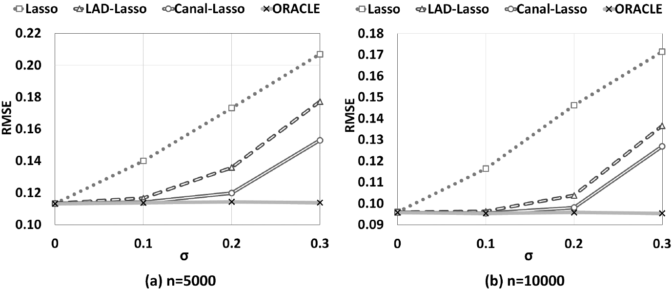
We investigate the proposed noise-resilient online regression algorithm on synthetic data sets in the case of noisy data. Specifically, we attempt to answer the question about how effective the proposed canal-LASSO method is in handling data with noise input and output. In this subsection, we have reported a number of simulation studies on finite-sample performance evaluation ( $n=$ 5000, 10000) of canal-LASSO on streaming noisy data. For comparison, LASSO, LAD-LASSO, canal-LASSO, together with the oracle estimator, are evaluated. Specifically, we set the feature dimension $d$ as 50 and let $\boldsymbol{\beta}$ be $(\underline{1,-2,3,-4,5,-6},0,0,\ldots,0)$ . Here, the first 6 regression coefficients are significant, while the remaining 44 regression coefficients are not. For a given $t$ , the covariate $\boldsymbol{x}_{t}$ is generated from a standard $d$ -dimensional multivariate normal distribution so that the components of $\boldsymbol{x}_{t}$ are independent and standard normal. Furthermore, the response variables are generated according to

$\displaystyle y_{t}=\boldsymbol{x}^{T}_{t}\boldsymbol{\beta}+\rho\epsilon_{t},$ (16)

where $\rho=$ 0.5 and $\epsilon_{t}$ is generated from normal distribution $N(0,1)$ . Here we change the noisy ratio $\sigma$ from $\{0,0.1,0.2,0.3\}$ . Specifically, we randomly select some samples $\{\boldsymbol{x}_{t},y_{t}\}$ at a rate of $\sigma$ and change the $6^{\text{th}}$ explanatory variable of $\boldsymbol{x}_{t}$ into 0 in the training set and then test the learning model in the true testing data set. We have reported the corresponding results in Table 4. At the same time, to explore the influence of noisy response variable, we randomly tamper the response variable $y$ to 0 at a rate of $\sigma$ in the training set and then test the learning model by the true testing samples. Corresponding results are reported in Table 5. For each parameter setting, a total of 50 random experiments are carried out to evaluate the average performance (for sample sizes $n$ equals 5000 and 10000, respectively). The absolute error of coefficient $D_{i}=|\frac{\hat{\beta_{i}}-\beta_{i}}{\beta_{i}}|$ , which stands for the normalized distance between estimated $\hat{\boldsymbol{\beta}}$ and true $\boldsymbol{\beta}$ is introduced to compare the capability of avoiding the interference from noisy response variable $y$ of different algorithms. The closer the $D_{i}$ is to 0, the higher accuracy of model coefficient estimation is. We list $D_{i}$ as an assessment criterion in Tables 4 and 5 to evaluate the learning models. For a fair comparison, the compared models, i.e., LASSO, LAD-LASSO and canal-LASSO are solved by the online gradient descent method (OGD). In our experiment, the parameter $\sigma$ is set to be 0.8.

We begin by demonstrating that the canal-LASSO is capable of avoiding the interference from explanatory variable $\boldsymbol{x}$ . As can be seen from the column of $D_{6}$ in Table 4, LASSO and LAD-LASSO deviate severely from true value and the proposed canal-LASSO method outperforms the two competing methods (LASSO, LAD-LASSO) in noisy data cases. Especially in the case of high noisy level ( $\sigma=$ 0.3), canal-LASSO significantly outperforms LASSO and LAD-LASSO. Due to the intrinsic flaw of $\ell_{2}$ loss, original LASSO method is very sensitive to noise. Least absolute deviation can reduce the impact of noise data in some sense, but the impact of noise remains seriously. The prediction performances of different algorithms are list in Fig. 5 for comprehensive comparison. As can be observed, the average performance of canal-LASSO outperforms LASSO and LAD-LASSO in noisy input cases. It indicates that canal-LASSO is indeed a noise-resilient method to deal with noisy data when the explanatory variables are contaminated.

Table 4

Simulation results for noisy covariate $\boldsymbol{x}$

n	$\sigma$	Method	$D_{1}$	$D_{2}$	$D_{3}$	$D_{4}$	$D_{5}$	$D_{6}$	$D_{\textit{total}}$	No. of zeros	$R^{2}$	RMSE
5000	0	LASSO	0.048	0.002	0.014	0.004	0.002	0.004	0.073	44 (100.0%)	0.9669	0.1135 $\pm$ 0.0008
		LAD-LASSO	0.042	0.011	0.022	0.005	0.010	0.004	0.093	43.95 (99.9%)	0.9664	0.1136 $\pm$ 0.0012
		canal-LASSO	0.040	0.013	0.023	0.009	0.008	0.002	0.095	44 (100.0%)	0.9669	0.1135 $\pm$ 0.0006
		ORACLE	0.000	0.000	0.000	0.000	0.000	0.000	0.000	44 (100.0%)	0.9670	0.1134 $\pm$ 0.0006
	0.1	LASSO	0.118	0.010	0.005	0.008	0.004	0.227	0.372	44 (100.0%)	0.9445	0.1244 $\pm$ 0.0007
		LAD-LASSO	0.075	0.008	0.005	0.008	0.004	0.089	0.188	44 (100.0%)	0.9573	0.1163 $\pm$ 0.0008
		canal-LASSO	0.072	0.008	0.006	0.004	0.009	0.069	0.169	44 (100.0%)	0.9590	0.1152 $\pm$ 0.0010
		ORACLE	0.000	0.000	0.000	0.000	0.000	0.000	0.000	44 (100.0%)	0.9608	0.1139 $\pm$ 0.0010
	0.2	LASSO	0.107	0.063	0.019	0.008	0.002	0.429	0.628	44 (100.0%)	0.8976	0.1473 $\pm$ 0.0016
		LAD-LASSO	0.040	0.035	0.034	0.009	0.034	0.185	0.336	44 (100.0%)	0.9479	0.1239 $\pm$ 0.0016
		canal-LASSO	0.039	0.028	0.023	0.009	0.020	0.135	0.254	44 (100.0%)	0.9542	0.1201 $\pm$ 0.0011
		ORACLE	0.000	0.000	0.000	0.000	0.000	0.000	0.000	44 (100.0%)	0.9620	0.1147 $\pm$ 0.0008
	0.3	LASSO	0.117	0.027	0.035	0.034	0.007	0.613	0.833	44 (100.0%)	0.8233	0.1724 $\pm$ 0.0021
		LAD-LASSO	0.057	0.056	0.031	0.021	0.042	0.319	0.525	43.6 (99.1%)	0.9211	0.1404 $\pm$ 0.0054
		canal-LASSO	0.103	0.037	0.027	0.028	0.027	0.218	0.441	42.85 (97.4%)	0.9425	0.1301 $\pm$ 0.0059
		ORACLE	0.000	0.000	0.000	0.000	0.000	0.000	0.000	44 (100.0%)	0.9676	0.1130 $\pm$ 0.0008
10000	0	LASSO	0.048	0.002	0.014	0.004	0.002	0.004	0.073	44 (100.0%)	0.9669	0.1135 $\pm$ 0.0008
		LAD-LASSO	0.014	0.006	0.002	0.007	0.010	0.002	0.041	44 (100.0%)	0.9593	0.0956 $\pm$ 0.0006
		canal-LASSO	0.025	0.018	0.005	0.007	0.003	0.004	0.062	44 (100.0%)	0.9590	0.0958 $\pm$ 0.0005
		ORACLE	0.000	0.000	0.000	0.000	0.000	0.000	0.000	44 (100.0%)	0.9591	0.0957 $\pm$ 0.0005
	0.1	LASSO	0.102	0.015	0.018	0.010	0.011	0.209	0.364	44 (100.0%)	0.9436	0.1041 $\pm$ 0.0007
		LAD-LASSO	0.056	0.006	0.002	0.003	0.008	0.043	0.117	44 (100.0%)	0.9596	0.0958 $\pm$ 0.0006
		canal-LASSO	0.065	0.010	0.003	0.002	0.005	0.018	0.102	44 (100.0%)	0.9607	0.0952 $\pm$ 0.0006
		ORACLE	0.000	0.000	0.000	0.000	0.000	0.000	0.000	44 (100.0%)	0.9610	0.0950 $\pm$ 0.0005
	0.2	LASSO	0.012	0.037	0.007	0.004	0.009	0.405	0.473	44 (100.0%)	0.8935	0.1245 $\pm$ 0.0009
		LAD-LASSO	0.020	0.022	0.018	0.006	0.021	0.094	0.181	44 (100.0%)	0.9580	0.0984 $\pm$ 0.0007
		canal-LASSO	0.032	0.050	0.020	0.018	0.009	0.040	0.168	44 (100.0%)	0.9615	0.0966 $\pm$ 0.0007
		ORACLE	0.000	0.000	0.000	0.000	0.000	0.000	0.000	44 (100.0%)	0.9626	0.0959 $\pm$ 0.0006
	0.3	LASSO	0.026	0.018	0.040	0.010	0.004	0.610	0.707	44 (100.0%)	0.8071	0.1467 $\pm$ 0.0008
		LAD-LASSO	0.065	0.065	0.031	0.052	0.024	0.227	0.464	43.7 (99.3%)	0.9408	0.1090 $\pm$ 0.0022
		canal-LASSO	0.023	0.059	0.037	0.033	0.005	0.095	0.251	43.8 (99.5%)	0.9600	0.0990 $\pm$ 0.0013
		ORACLE	0.000	0.000	0.000	0.000	0.000	0.000	0.000	44 (100.0%)	0.9660	0.0951 $\pm$ 0.0006

Table 5

Simulation results for noisy response variable $y$

n	$\sigma$	Method	$D_{1}$	$D_{2}$	$D_{3}$	$D_{4}$	$D_{5}$	$D_{6}$	$D_{\textit{total}}$	No. of zeros	$R^{2}$	RMSE
5000	0	LASSO	0.092	0.011	0.003	0.007	0.013	0.011	0.137	44 (100.0%)	0.9626	0.1133 $\pm$ 0.0013
		LAD-LASSO	0.084	0.007	0.006	0.004	0.014	0.009	0.124	44 (100.0%)	0.9622	0.1135 $\pm$ 0.0009
		canal-LASSO	0.079	0.015	0.005	0.006	0.014	0.006	0.124	44 (100.0%)	0.9625	0.1132 $\pm$ 0.0007
		ORACLE	0.000	0.000	0.000	0.000	0.000	0.000	0.000	44 (100.0%)	0.9626	0.1131 $\pm$ 0.0007
	0.1	LASSO	0.242	0.153	0.180	0.254	0.207	0.194	1.230	43.95 (99.9%)	0.9202	0.1399 $\pm$ 0.0020
		LAD-LASSO	0.063	0.023	0.045	0.049	0.048	0.035	0.263	43.95 (99.9%)	0.9623	0.1166 $\pm$ 0.0037
		canal-LASSO	0.048	0.008	0.017	0.016	0.017	0.004	0.109	44 (100.0%)	0.9658	0.1141 $\pm$ 0.0009
		ORACLE	0.000	0.000	0.000	0.000	0.000	0.000	0.000	44 (100.0%)	0.9662	0.1137 $\pm$ 0.0009
	0.2	LASSO	0.752	0.361	0.331	0.441	0.401	0.416	2.703	43.25 (98.3%)	0.7981	0.1732 $\pm$ 0.0027
		LAD-LASSO	0.334	0.164	0.136	0.222	0.169	0.178	1.202	43.15 (98.1%)	0.9235	0.1358 $\pm$ 0.0055
		canal-LASSO	0.174	0.067	0.059	0.112	0.065	0.066	0.543	43.55 (99.0%)	0.9537	0.1198 $\pm$ 0.0026
		ORACLE	0.000	0.000	0.000	0.000	0.000	0.000	0.000	44 (100.0%)	0.9618	0.1143 $\pm$ 0.0007
	0.3	LASSO	1.000	0.669	0.627	0.602	0.603	0.610	4.112	43.15 (98.1%)	0.5871	0.2069 $\pm$ 0.0036
		LAD-LASSO	0.686	0.461	0.343	0.464	0.415	0.413	2.782	41.6 (94.5%)	0.7774	0.1772 $\pm$ 0.0058
		canal-LASSO	0.668	0.346	0.167	0.325	0.228	0.261	1.996	40.3 (91.6%)	0.8664	0.1529 $\pm$ 0.0184
		ORACLE	0.000	0.000	0.000	0.000	0.000	0.000	0.000	44 (100.0%)	0.9625	0.1137 $\pm$ 0.0008
10000	0	LASSO	0.041	0.004	0.004	0.007	0.004	0.010	0.070	44 (100.0%)	0.9592	0.0960 $\pm$ 0.0006
		LAD-LASSO	0.039	0.003	0.008	0.008	0.003	0.011	0.072	44 (100.0%)	0.9590	0.0959 $\pm$ 0.0004
		canal-LASSO	0.055	0.008	0.007	0.002	0.006	0.012	0.090	44 (100.0%)	0.9596	0.0958 $\pm$ 0.0005
		ORACLE	0.000	0.000	0.000	0.000	0.000	0.000	0.000	44 (100.0%)	0.9597	0.0958 $\pm$ 0.0005
	0.1	LASSO	0.259	0.202	0.204	0.199	0.189	0.211	1.264	44 (100.0%)	0.9172	0.1164 $\pm$ 0.0014
		LAD-LASSO	0.013	0.044	0.029	0.032	0.023	0.029	0.169	44 (100.0%)	0.9610	0.0963 $\pm$ 0.0007
		canal-LASSO	0.033	0.007	0.010	0.005	0.003	0.001	0.059	44 (100.0%)	0.9622	0.0954 $\pm$ 0.0004
		ORACLE	0.000	0.000	0.000	0.000	0.000	0.000	0.000	44 (100.0%)	0.9623	0.0953 $\pm$ 0.0004
	0.2	LASSO	0.881	0.383	0.420	0.408	0.411	0.421	2.923	43.7 (99.3%)	0.7651	0.1462 $\pm$ 0.0016
		LAD-LASSO	0.134	0.075	0.151	0.129	0.120	0.110	0.718	43.6 (99.1%)	0.9399	0.1039 $\pm$ 0.0014
		canal-LASSO	0.055	0.021	0.104	0.054	0.062	0.032	0.328	43.3 (98.4%)	0.9526	0.0981 $\pm$ 0.0016
		ORACLE	0.000	0.000	0.000	0.000	0.000	0.000	0.000	44 (100.0%)	0.9569	0.0958 $\pm$ 0.0006
	0.3	LASSO	0.855	0.624	0.609	0.587	0.595	0.606	3.876	42.9 (97.5%)	0.5231	0.1714 $\pm$ 0.0020
		LAD-LASSO	0.596	0.286	0.329	0.303	0.325	0.390	2.229	40.2 (91.4%)	0.8066	0.1366 $\pm$ 0.0044
		canal-LASSO	0.464	0.205	0.216	0.236	0.292	0.334	1.747	41.4 (94.1%)	0.8536	0.1269 $\pm$ 0.0086
		ORACLE	0.000	0.000	0.000	0.000	0.000	0.000	0.000	44 (100.0%)	0.9544	0.0954 $\pm$ 0.0005

Figure 5.

Simulation results for noisy covariate $\boldsymbol{x}$ .

When response variable $\boldsymbol{y}$ are contaminated, each coefficient may be affected. Considering the overall impact of noise $y$ , we focus on $D_{\textit{total}}=\sum^{6}_{1}D_{i}$ that emphasizes the overall variation of $\boldsymbol{\beta}$ . As can be seen from the column of $D_{\textit{total}}$ in Table 5, the proposed canal-LASSO outperforms the two competing methods (LASSO, LAD-LASSO) significantly in noisy data cases. Due to the least square deviation, original LASSO method is very sensitive to noise data. For the estimation of $\beta_{1-6}$ , LASSO deviate severely from true value coefficient $\boldsymbol{\beta}$ than LAD-LASSO and canal-LASSO. Compared to least square deviation, least absolute deviation (LAD) can effectively reduce the impact of noise data, but the negative impact of noise is still serious. To compare the models more comprehensively, the prediction performances of different models are listed in Fig. 6. As can be observed, the average performance of canal-LASSO outperforms LASSO and LAD-LASSO in noisy output cases. It indicates that canal-LASSO is a noise-resilient method to deal with noisy data when the response variable $y$ is contaminated.

Table 6

Details of benchmark datasets

Dataset	#Samples	#Features	#Train number	#Test number
Kin	3000 $\times$ 3	8	2100 $\times$ 3	900 $\times$ 3
Abalone	4177 $\times$ 3	7	2924 $\times$ 3	1253 $\times$ 3
Letters	5000 $\times$ 3	15	3500 $\times$ 3	1500 $\times$ 3
Pendigits	7129 $\times$ 3	14	4990 $\times$ 3	2139 $\times$ 3

Table 7

Parameter setting of canal loss for four benchmark datasets

Dataset	Kin	Abalone	Letters	Pendigits
$\zeta$	0.1	0.1	0.1	0.1
$\gamma$	1.2	1.4	1.6	1.6

Figure 6.

Simulation results for noisy response variable $y$ .

4.3 Benchmark data sets

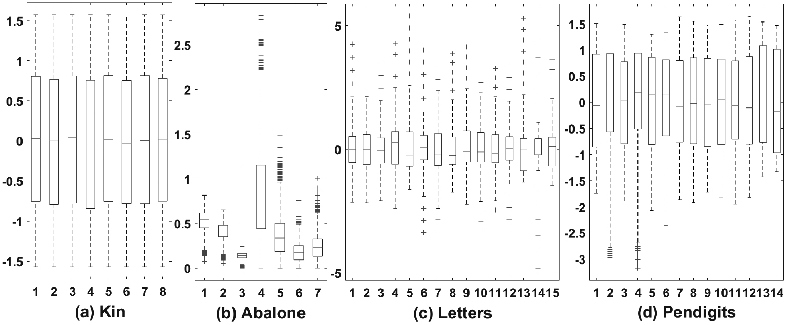
In this subsection, we conduct extensive experiments to evaluate the performance of the proposed online canal-LASSO algorithm on linear regression tasks. Four benchmark datasets including “Kin”, “Abalone”, “Letters” and “Pendigits” are used for the experimental evaluation. Details of the datasets used in this experiment are listed in Table 6. In order to show the statistical properties of different data sets, we drew a box plot as shown in Fig. 7. Before the experiment, the parameter sensitivity of our model should be analyzed and designated by domain expert according to the parameter sensitivity study in Section 4.1. For four benchmark datasets, our parameter settings are shown in Table 7. To simulate the setting of streaming data, we duplicate the samples by three times. Additionally, all the experiments are randomly performed 20 times repeatedly and the average performance is reported.

Table 8
Experimental results on benchmark datasets

Dataset	$\sigma$	Method	RMSE	MAE	Discarded samples		Discarded rate	Time (s)
Kin	0	LASSO	0.0715 $\pm$ 0.0006	0.2166 $\pm$ 0.0049	0	$\pm$ 0	0.0%	0.3676 $\pm$ 0.0677
		LAD-LASSO	0.0720 $\pm$ 0.0004	0.2208 $\pm$ 0.0033	0	$\pm$ 0	0.0%	0.3854 $\pm$ 0.0416
		canal-LASSO	0.0719 $\pm$ 0.0003	0.2199 $\pm$ 0.0026	657	$\pm$ 22	7.3%	0.3829 $\pm$ 0.0259
	0.1	LASSO	0.0730 $\pm$ 0.0006	0.2238 $\pm$ 0.0034	0	$\pm$ 0	0.0%	0.3797 $\pm$ 0.0692
		LAD-LASSO	0.0720 $\pm$ 0.0006	0.2188 $\pm$ 0.0036	0	$\pm$ 0	0.0%	0.4057 $\pm$ 0.0762
		canal-LASSO	0.0718 $\pm$ 0.0005	0.2199 $\pm$ 0.0039	1499	$\pm$ 32	16.7%	0.4028 $\pm$ 0.0636
	0.2	LASSO	0.0764 $\pm$ 0.0009	0.2453 $\pm$ 0.0065	0	$\pm$ 0	0.0%	0.3532 $\pm$ 0.0213
		LAD-LASSO	0.0736 $\pm$ 0.0006	0.2270 $\pm$ 0.0037	0	$\pm$ 0	0.0%	0.3716 $\pm$ 0.0184
		canal-LASSO	0.0718 $\pm$ 0.0005	0.2200 $\pm$ 0.0037	2337	$\pm$ 24	26.0%	0.3717 $\pm$ 0.0246
	0.3	LASSO	0.0806 $\pm$ 0.0004	0.2732 $\pm$ 0.0022	0	$\pm$ 0	0.0%	0.3607 $\pm$ 0.0186
		LAD-LASSO	0.0771 $\pm$ 0.0010	0.2490 $\pm$ 0.0064	0	$\pm$ 0	0.0%	0.3714 $\pm$ 0.0225
		canal-LASSO	0.0720 $\pm$ 0.0003	0.2202 $\pm$ 0.0024	3171	$\pm$ 21	35.2%	0.3752 $\pm$ 0.0238
Abalone	0	LASSO	0.2261 $\pm$ 0.0016	2.3521 $\pm$ 0.0295	0	$\pm$ 0	0.0%	0.5315 $\pm$ 0.0336
		LAD-LASSO	0.2290 $\pm$ 0.0020	2.3600 $\pm$ 0.0420	0	$\pm$ 0	0.0%	0.5562 $\pm$ 0.0217
		canal-LASSO	0.2281 $\pm$ 0.0021	2.3735 $\pm$ 0.0390	1349	$\pm$ 31	10.8%	0.5628 $\pm$ 0.0241
	0.1	LASSO	0.2333 $\pm$ 0.0029	2.3884 $\pm$ 0.0572	0	$\pm$ 0	0.0%	0.5433 $\pm$ 0.0263
		LAD-LASSO	0.2321 $\pm$ 0.0022	2.3813 $\pm$ 0.0353	0	$\pm$ 0	0.0%	0.5697 $\pm$ 0.0242
		canal-LASSO	0.2280 $\pm$ 0.0022	2.3945 $\pm$ 0.0433	2516	$\pm$ 39	20.1%	0.5655 $\pm$ 0.0284
	0.2	LASSO	0.2516 $\pm$ 0.0026	2.7840 $\pm$ 0.0578	0	$\pm$ 0	0.0%	0.5315 $\pm$ 0.0236
		LAD-LASSO	0.2358 $\pm$ 0.0020	2.4291 $\pm$ 0.0490	0	$\pm$ 0	0.0%	0.5782 $\pm$ 0.0265
		canal-LASSO	0.2300 $\pm$ 0.0015	2.4129 $\pm$ 0.0288	3681	$\pm$ 22	29.4%	0.5664 $\pm$ 0.0163
	0.3	LASSO	0.2652 $\pm$ 0.0039	3.1682 $\pm$ 0.1161	0	$\pm$ 0	0.0%	0.5546 $\pm$ 0.0356
		LAD-LASSO	0.2411 $\pm$ 0.0029	2.4951 $\pm$ 0.0702	0	$\pm$ 0	0.0%	0.5766 $\pm$ 0.0164
		canal-LASSO	0.2292 $\pm$ 0.0033	0.2202 $\pm$ 0.0024	4863	$\pm$ 23	38.8%	0.5720 $\pm$ 0.0422
Letters	0	LASSO	0.3345 $\pm$ 0.0011	6.5444 $\pm$ 0.0443	0	$\pm$ 0	0.0%	0.7345 $\pm$ 0.0299
		LAD-LASSO	0.3310 $\pm$ 0.0009	6.3388 $\pm$ 0.0633	0	$\pm$ 0	0.0%	0.7462 $\pm$ 0.0442
		canal-LASSO	0.3321 $\pm$ 0.0009	6.3192 $\pm$ 0.0474	1307	$\pm$ 22	8.7%	0.7475 $\pm$ 0.0281
	0.1	LASSO	0.3370 $\pm$ 0.0011	6.6093 $\pm$ 0.0458	0	$\pm$ 0	0.0%	0.7240 $\pm$ 0.0296
		LAD-LASSO	0.3360 $\pm$ 0.0017	6.4904 $\pm$ 0.0745	0	$\pm$ 0	0.0%	0.7664 $\pm$ 0.0619
		canal-LASSO	0.3349 $\pm$ 0.0017	6.4423 $\pm$ 0.0878	2684	$\pm$ 25	17.9%	0.7280 $\pm$ 0.0282
	0.2	LASSO	0.3441 $\pm$ 0.0024	6.7572 $\pm$ 0.1015	0	$\pm$ 0	0.0%	0.7146 $\pm$ 0.0257
		LAD-LASSO	0.3519 $\pm$ 0.0014	6.9318 $\pm$ 0.0622	0	$\pm$ 0	0.0%	0.7539 $\pm$ 0.0587
		canal-LASSO	0.3404 $\pm$ 0.0017	6.6541 $\pm$ 0.0806	4496	$\pm$ 35	30.0%	0.7429 $\pm$ 0.0455
	0.3	LASSO	0.3561 $\pm$ 0.0026	7.1115 $\pm$ 0.1078	0	$\pm$ 0	0.0%	0.7183 $\pm$ 0.0343
		LAD-LASSO	0.3764 $\pm$ 0.0021	7.6620 $\pm$ 0.1152	0	$\pm$ 0	0.0%	0.7700 $\pm$ 0.0372
		canal-LASSO	0.3419 $\pm$ 0.0019	6.7535 $\pm$ 0.0791	5386	$\pm$ 22	35.9%	0.7556 $\pm$ 0.0368
Pendigits	0	LASSO	0.1898 $\pm$ 0.0005	2.5112 $\pm$ 0.0199	0	$\pm$ 0	0.0%	1.2365 $\pm$ 0.0474
		LAD-LASSO	0.1875 $\pm$ 0.0007	2.4515 $\pm$ 0.0324	0	$\pm$ 0	0.0%	1.2491 $\pm$ 0.0335
		canal-LASSO	0.1884 $\pm$ 0.0008	2.4805 $\pm$ 0.0285	2497	$\pm$ 25	10.2%	1.2647 $\pm$ 0.0544
	0.1	LASSO	0.1914 $\pm$ 0.0009	2.5208 $\pm$ 0.0273	0	$\pm$ 0	0.0%	1.2485 $\pm$ 0.0296
		LAD-LASSO	0.1895 $\pm$ 0.0010	2.4600 $\pm$ 0.0285	0	$\pm$ 0	0.0%	1.2697 $\pm$ 0.0733
		canal-LASSO	0.1880 $\pm$ 0.0011	2.4776 $\pm$ 0.0373	4365	$\pm$ 15	17.8%	1.2541 $\pm$ 0.0370
	0.2	LASSO	0.1936 $\pm$ 0.0005	2.5733 $\pm$ 0.0123	0	$\pm$ 0	0.0%	1.2719 $\pm$ 0.0629
		LAD-LASSO	0.1973 $\pm$ 0.0010	2.5898 $\pm$ 0.0293	0	$\pm$ 0	0.0%	1.3072 $\pm$ 0.0983
		canal-LASSO	0.1871 $\pm$ 0.0008	2.4594 $\pm$ 0.0247	6271	$\pm$ 16	25.5%	1.2847 $\pm$ 0.0636
	0.3	LASSO	0.1992 $\pm$ 0.0011	2.6751 $\pm$ 0.0226	0	$\pm$ 0	0.0%	1.2328 $\pm$ 0.0375
		LAD-LASSO	0.2124 $\pm$ 0.0023	2.9270 $\pm$ 0.0649	0	$\pm$ 0	0.0%	1.2500 $\pm$ 0.0431
		canal-LASSO	0.1874 $\pm$ 0.0009	2.4696 $\pm$ 0.0315	8130	$\pm$ 14	33.1%	1.2756 $\pm$ 0.0587

Figure 7.

Box plots of four benchmark datasets.

Figure 8.

Experimental results on benchmark datasets.

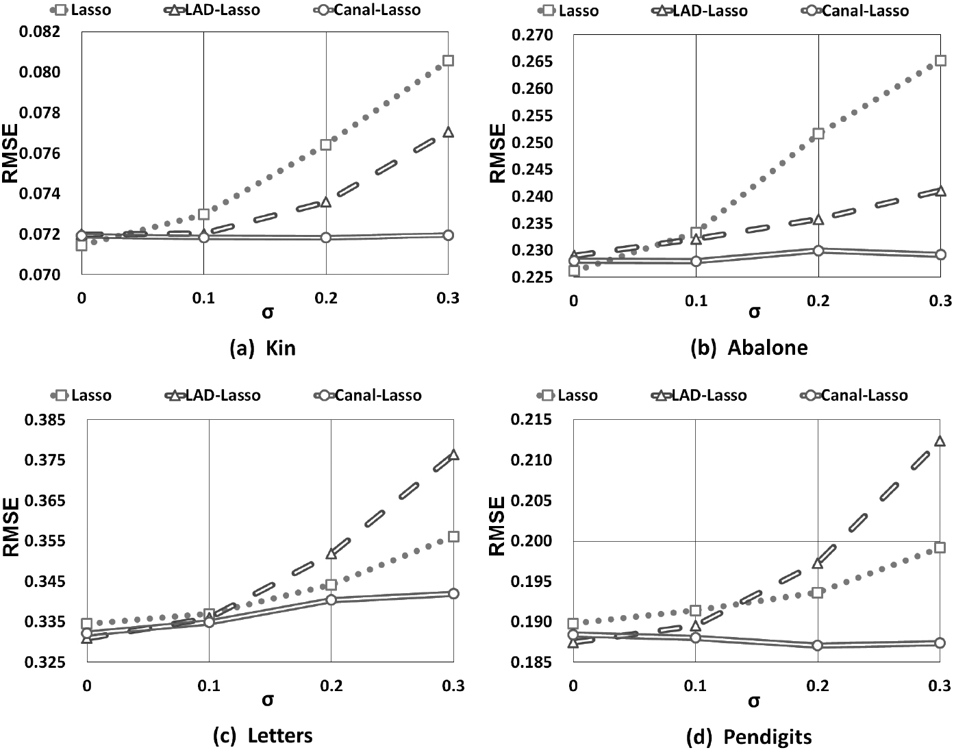
Table 8 shows the running time, discarded rate and the regression accuracy (RMSE and MAE) of three compared methods, i.e., LASSO, LAD-LASSO, and canal-LASSO on the benchmark datasets. The column of RMSE and MAE show that the performance of three compared methods is similar when data is clean ( $\sigma=$ 0). But in the scenario of noisy data ( $\sigma=$ 0.1, 0.2 and 0.3), the proposed canal-LASSO outperforms LASSO and LAD-LASSO. Moreover, the performance of canal-LASSO is steady in both cases of clean data and noisy data. The column of discarded rate shows that the only partial of learning samples are learned by the canal-LASSO model. The discarded rate increases according to the noise level parameter $\sigma$ . As the running time is concerned, thanks to the efficient OGD framework, it can be observed that LASSO, LAD-LASSO and canal-LASSO only takes little running time. To have a more comprehensive comparison, we show the average RMSE in Fig. 8. On datasets “Kin” and “Abalone”, LASSO is more sensitive to noise. However, on datasets “Letters” and “Pendigits”, LAD-LASSO is more sensitive to noisy data. The proposed canal-LASSO is the most stable one on all of the four datasets, so it is a good candidate to deal with noisy data streams.

5. Conclusion

In this work, we have studyed a novel problem of online learning from noisy data streams and proposed a linear regression model canal-LASSO. Furthermore, an efficient algorithm based on the online gradient descend framework is presented to solve canal-LASSO. Simulated experiments have shown that the proposed canal-LASSO is noise-resilient in the scenarios of both noisy covariate $\boldsymbol{x}$ and response variable $\boldsymbol{y}$ . At last, we have conducted extensive experiments on benchmark datasets to validate that canal-LASSO is robust and a good candidate to deal with noisy data streams. Future work will involve extending the linear regression model to non-linear regression model by the introducing of kernel trick [38].

Footnotes

Acknowledgments

This work was supported by the National Natural Science Foundation of China under Grant No. 61873279, National Key Research and Development Program of Shandong Province under Grant No. 2018GSF120020, National Natural Science Foundation of Shandong Province under Grant No. ZR2019MA016, and Fundamental Research Funds for the Central Universities under Grant No. 20CX05003B.

References

Meinshausen

and Bühlmann

, Stability selection, Journal of the Royal Statistical Society: Series B (Statistical Methodology) 72(4) (2010), 417–473.

Tibshirani

, Regression shrinkage and selection via the lasso, Journal of the Royal Statistical Society 58(1) (1996), 267–288.

Fan

and Li

, Variable selection via nonconcave penalized likelihood and its oracle properties, Journal of the American Statistical Association 96(456) (2001), 1348–1360.

Zou

, The adaptive lasso and its oracle properties, Journal of the American Statistical Association 101(476) (2006), 1418–1429.

Bloomfield

and Steiger

W.L.

, Least absolute deviations: Theory, applications and algorithms, Springer, 1984.

Wang

and Jiang

, Robust regression shrinkage and consistent variable selection through the lad-lasso, Journal of Business & Amp; Economic Statistics 25(3) (2007), 347–355.

Bottou

, Large-scale machine learning with stochastic gradient descent, in: Proceedings of COMPSTAT’2010, Springer, 2010, pp. 177–186.

Ditzler

Roveri

Alippi

and Polikar

, Learning in nonstationary environments: A survey, IEEE Computational Intelligence Magazine 10(4) (2015), 12–25.

Sun

and Huang

, A stable online scheduling strategy for real-time stream computing over fluctuating big data streams, IEEE Access 4 (2016), 8593–8607.

10.

Aggarwal

C.C.

, Data streams: models and algorithms, Vol. 31, Springer Science & Amp; Business Media, 2007.

11.

Gama

, Knowledge discovery from data streams, Intelligent Data Analysis 13(3) (2009), 403–404.

12.

Jian

and Liu

, Toward online node classification on streaming networks, Data Mining and Knowledge Discovery 32(1) (2018), 231–257.

13.

Jian

Gao

Ren

Song

and Luo

, A noise-resilient online learning algorithm for scene classification, Remote Sensing 10(11) (2018), 1836.

14.

LeoBreiman, Better subset regression using the nonnegative garrote, Technometrics 37(4) (1995), 373–384.

15.

Hastie

and Mallows

, A statistical view of some chemometrics regression tools: Discussion, Technometrics 35(2) (1993), 140–143.

16.

Zhang

C.H.

, Nearly unbiased variable selection under minimax concave penalty, Annals of Statistics 38(2) (2010), 894–942.

17.

Zou

and Hastie

, Regularization and variable selection via the elastic net, Journal of the Royal Statistical Society: Series B (Statistical Methodology) 67(2) (2005), 301–320.

18.

Yuan

and Lin

, Model selection and estimation in regression with grouped variables, Journal of the Royal Statistical Society: Series B (Statistical Methodology) 68(1) (2006), 49–67.

19.

Wang

Jiang

Huang

and Zhang

, Robust variable selection with exponential squared loss, Journal of the American Statistical Association 108(502) (2013), 632–643.

20.

Chang

Roberts

and Welsh

, Robust lasso regression using tukey’s biweight criterion, Technometrics 60(1) (2018), 36–47.

21.

and Zhang

C.-X.

, Robust sparse regression by modeling noise as a mixture of gaussians, Journal of Applied Statistics 46(10) (2019), 1738–1755.

22.

Zurada

J.M.

, Introduction to artificial neural systems, Vol. 8, West publishing company St. Paul, 1992.

23.

Bhadeshia

, Neural networks and information in materials science, Statistical Analysis and Data Mining: The ASA Data Science Journal 1(5) (2009), 296–305.

24.

Gunn

S.R.

et al., Support vector machines for classification and regression, ISIS Technical Report 14(1) (1998), 5–16.

25.

Wang

and Vucetic

, Online training on a budget of support vector machines using twin prototypes, Statistical Analysis and Data Mining: The ASA Data Science Journal 3(3) (2010), 149–169.

26.

Aggarwal

C.C.

, Data mining: the textbook, Springer, 2015.

27.

Bottou

, Online learning and stochastic approximations, On-line Learning in Neural Networks 17(9) (1998), 142.

28.

Arce

and Salinas

, Online ridge regression method using sliding windows, in: Chilean Computer Science Society (SCCC), 2012 31st International Conference of the, IEEE, 2012, pp. 87–90.

29.

Gao

Song

Jian

and Liang

, Toward budgeted online kernel ridge regression on streaming data, IEEE Access 7 (2019), 26136–26145.

30.

Monti

R.P.

Anagnostopoulos

and Montana

, Adaptive regularization for lasso models in the context of nonstationary data streams, Statistical Analysis and Data Mining: The ASA Data Science Journal 11(5) (2018), 237–247.

31.

Orabona

Keshet

and Caputo

, The projectron: a bounded kernel-based perceptron, in: Proceedings of the 25th International Conference on Machine Learning, ACM, 2008, pp. 720–727.

32.

Zhao

Wang

Jin

and Hoi

S.C.

, Fast bounded online gradient descent algorithms for scalable kernel-based online learning, arXiv preprint arXiv:1206.4633.

33.

Garrigues

and Ghaoui

L.E.

, An homotopy algorithm for the lasso with online observations, in: Advances in Neural Information Processing Systems, 2009, pp. 489–496.

34.

Huang

Shi

and Suykens

J.A.

, Ramp loss linear programming support vector machine, The Journal of Machine Learning Research 15(1) (2014), 2185–2211.

35.

Robbins

and Monro

, A stochastic approximation method, The Annals of Mathematical Statistics (1951), 400–407.

36.

Blake

and Merz

, Uci repository of machine learning databases, department of information and computer science, University of California, Irvine, CA 55.

37.

Chang

C.-C.

and Lin

C.-J.

, Libsvm: A library for support vector machines, ACM Transactions on Intelligent Systems and Technology (TIST) 2(3) (2011), 27.

38.

Liu

Pokharel

P.P.

and Principe

J.C.

, The kernel least-mean-square algorithm, IEEE Transactions on Signal Processing 56(2) (2008), 543–554.

Canal-LASSO: A sparse noise-resilient online linear regression model

Abstract

Keywords

1. Introduction

3.1 Canal-LASSO

1 Available: http://archive.ics.uci.edu/ml/.

3 Henceforth we use the same proportion for all of the datasets.

Table 8 Experimental results on benchmark datasets

Footnotes

Acknowledgments

References

¹
Available: http://archive.ics.uci.edu/ml/.

³
Henceforth we use the same proportion for all of the datasets.

Table 8
Experimental results on benchmark datasets