An efficient method for time series similarity search using binary code representation and hamming distance

Abstract

Time series similarity search is an essential operation in time series data mining and has received much higher interest along with the growing popularity of time series data. Although many algorithms to solve this problem have been investigated, there is a challenging demand for supporting similarity search in a fast and accurate way. In this paper, we present a novel approach, TS2BC, to perform time series similarity search efficiently and effectively. TS2BC uses binary code to represent time series and measures the similarity under the Hamming Distance. Our method is able to represent original data compactly and can handle shifted time series and work with time series of different lengths. Moreover, it can be performed with reasonably low complexity due to the efficiency of calculating the Hamming Distance. We extensively compare TS2BC with state-of-the-art algorithms in classification framework using 61 online datasets. Experimental results show that TS2BC achieves better or comparative performance than other the state-of-the-art in accuracy and is much faster than most existing algorithms. Furthermore, we propose an approximate version of TS2BC to speed up the query procedure and test its efficiency by experiment.

Keywords

1. Introduction

A time series is a sequence of real numbers, each of which represents a value measured at a point in time. In recent years, time series have extended to many scientific and social domains, including medicine [1], economics [2], engineering fields [3], and so on. With the growing popularity of time series data, there are various kinds of time series related research, an important one which has received an increasing amount of attention lately is the similarity search in time series databases.

Similarity search is of great significance for time series prediction [4], clustering [5], classification [6] and knowledge discovery [7]. Therefore, the problem of time series similarity search has been the focus of many research activities in the data mining community for the past few years. A multitude of methods have been proposed [8, 9, 10, 11]. Most of them can be classified as one of two types [11]:

•
Time series representation. Time series are always high-dimensional data. Therefore, working directly on the raw data requires a lot of computing resources and storage space. Thus, representing a time series in a concise form is an essential step of time series similarity search. Additional benefits gained are efficient storage, speedup of processing, as well as implicit noise removal [12]. The ideal representation method should be computationally efficient and significantly reduce data dimensionality. Besides, it should be able to maintain the essential characteristics of the raw data.
•
Similarity measure. The similarity measure is of fundamental importance for a variety of time series analysis and data mining tasks. Most time series analysis techniques, including clustering, classification and querying, critically depend on the choice of similarity measure. However, devising a similarity function in the time series domain is by no means trivial. It should be consistent with human intuition and can consider the most salient features on both local and global scales. Moreover, similarity measure should be performed with reasonably low complexity.

Although many representation techniques and similarity measures have been investigated, most of them can not solve the problem of time series similarity search perfectly, due to some basic requirements which should be satisfied by all methods.

•
Low computational cost. Time series are mostly high-dimensional data. Therefore, a method should be performed with low computational complexity for computing the representation or similarity measure.
•
Capability to handle shifted time series. Commonly, time series in a database are shifted in the time axis [13]. From the perspective of human cognition, two shifted time series are very similar to each other. However, not all similarity measures can handle this type of similarity.
•
Capability to deal with time series of unequal lengths. Some algorithms can only address time series of the same length. However, in practical scenarios, most of the time series are not equal in length, which leads to severe limitations for these algorithms in practical applications.

Each proposed method offers different trade-offs between the requirements listed above. For example, the Euclidean Distance and, in general, $L_{p}$ norms [14] can be calculated in linear time. However, when the lengths of two time series are different or when it is required to match series that are locally out of phase, using Euclidean Distance may not produce the desired results [15]. In such cases, a more robust similarity measure named Dynamic Time Warping [16], is used instead. Nevertheless, it has a quadratic time and space complexity, which is computationally expensive.

Based on the above requirements, in this paper, we propose a novel method named TS2BC (Time Series to Binary Code) to address the problem of the time series similarity search. TS2BC models time series as points on a plane and divides the plane into several cells. Then, by recording the cells through which the time series pass, the algorithm transforms time series into binary codes. This bit-level representation method has several advantages over existing methods [17]. First, binary codes are storage efficient and can be efficiently manipulated. Secondly, the bit-level representation allows us to use many available algorithms that are applicable to binary code only [18, 19]. With the generated binary codes, TS2BC uses Hamming Distance to measure the similarity between the pairwise time series. We emphasize that the Hamming Distance computation is extremely fast on modern CPUs, specifically, according to [20], 50 $\sim$ 100 speedups can be achieved if we calculate the similarity by Hamming Distance instead of Euclidean Distance.

TS2BC is devised based on the intuition that similar time series always pass through similar cells in a plane. It is consistent with human cognition and can be applied to different kinds of datasets. TS2BC can handle shifted time series and remove the effects of noise and missing values by using appropriate parameters and can deal with time series of unequal lengths. Besides, it has low computational complexity to calculate the representation and similarity measure.

The main contributions of our work are as follows:

•
We propose a novel approach, TS2BC, which can handle time series similarity search efficiently by transforming time series into binary codes in linear time and using Hamming Distance to measure the similarity between pairwise time series.
•
We present an approximate version of TS2BC (ATS2BC) to speed our approach up because there are many situations in which a user would be willing to sacrifice some accuracy for a significant speedup.
•
To demonstrate the efficiency and effectiveness of the proposed approach, we conduct extensive experiments on public datasets by using classification frameworks. Experimental results show that our proposed method can achieve better or comparative performance in accuracy than other state-of-the-art algorithms, and can achieve much higher efficiency than most existing algorithms.

The rest of the paper is organized as follows. Section 2 introduces the related works on time series representation methods and similarity measures. Section 3 presents the TS2BC algorithm in detail and Section 4 discusses some important aspects of TS2BC. Approximate version of the TS2BC can be found in Section 5. Section 6 shows the experimental results. Finally, the paper is concluded in Section 7.
2. Related works

Time series similarity search is mainly studied in two aspects, time series representation and similarity measure. In this section, we briefly introduce the representation methods and similarity measures.

2.1 Time series representations

Representing a time series in a concise form that can be effectively processed is an essential step of time series similarity search.

Piecewise Aggregate Approximate (PAA) [21] reduces the time series from $n$ dimensions to $N(N<n)$ dimensions by dividing time series into $N$ equal-length segments. The mean value of the time series falling within a segment is recorded, and a vector of these values becomes the data reduced representation. PAA is simple and fast to compute but can only handle segments with the same length and may miss some information such as maximums or minimums. Based on PAA, literature [22] presents an extended version called Adaptive Piecewise Constant Approximate (APCA), in which the length of each segment is not fixed, but adaptive to the shape of the series. APCA outperforms the original PAA, and it also creates a better approximation for time-series. Piecewise Linear Approximate (PLA) [23] is another approach to reduce the dimension of time series data. It attempts to model the time series as sequences of straight lines. Many derivatives of this method have been introduced [24, 25]. Another common family of time series representation methods convert the numeric time series to symbolic form. For example, Symbolic Aggregate approxiMation (SAX) [26], based on PAA, applies a further transformation to obtain a discrete representation after transforming a time series into PAA. All PAA coefficients can be transformed into some discrete strings by breakpoints [26]. Indexable Symbolic Aggregate approXimation (iSAX) [27] is an extension of this approach, which can make fast indexing possible. Similar to our method, a technique called clipping [28] also converts a time series to a binary code. Each bit in the binary code indicates whether the series is above or below the average.

Most of the techniques described so far are representing time series data in the time domain directly. Representing time series in the transformation domain is another large family of methods. These commonly used representations include Discrete Fourier Transform (DFT) [29], Single Value Decomposition (SVD) [30], Discrete Wavelet Transform (DWT) [31], and Chebyshev Polynomials (CP) [32].

Recently, in [9], the authors present an algorithm named STS3, which can transform time series into sets. It is the first work using set techniques to accelerate time series search. Inspired by the idea of STS3, in this work, we present a binary code-based representation method for time series. The STS3 algorithm has played a significant role in the design of our method and will be discussed at greater depth in Sections 4.1 and 6.2.

2.2 Time series similarity measures

The similarity measure is a significant aspect of similarity search in time series data mining. Given two time series $T_{1}$ and $T_{2}$ , the similarity measure $\textit{Dist}(T_{1},T_{2})$ calculates the distance between them. Almost every time series mining task requires a notion of similarity between two time series.

The simplest way to estimate the similarity between two time series is the lock-step measure [14], which compares the $i$ th point of one time series to the $i$ th point of another. For example, Euclidean Distance (ED), along with its variants based on the common $L_{p}$ -norms. Lock-step measures have several advantages. An important one is that the complexity of evaluating these measures is $O(n)$ , where $n$ is the length of the time series, and they are easy to implement and, besides, they are parameter-free. Furthermore, it should be noted that, the ED is surprisingly competitive with the other, more sophisticated methods, especially in the case of very large datasets. However, these similarity measures can only handle time series with the same length and are very sensitive to noise and temporal warping.

Unlike the lock-step measure, elastic measure allows comparison of one-to-many/one-to-none points. For example, Dynamic Time Warping (DTW) [16] is a classic elastic measure for executing similarity search in time series. DTW is more robust than ED and can handle shifted time series and time series with different lengths. DTW has been successfully used for time series similarity search and shown to be very hard to beat [33, 34, 14]. It can be computed using dynamic programming with time complexity $O(n^{2})$ , which is computationally too expensive, especially for long time series. DTW is a hot study domain and many techniques have been proposed for improving its performance, for example: Weighted DTW [35], shapeDTW [36], Locally Slope-based DTW [37] and Derivative DTW [38]. We refer readers to [36] to see more derivatives of this approach. Other elastic measures include Longest Common Subsequences (LCSS) [39], Edit Distance with Real Penalty (ERP) [40] and Edit Distance on Real Sequence (EDR) [41]. It should be noted that all of these methods are of computational complexity $O(n^{2})$ .

Based on the proposed binary code-based representation method, in this paper, a matching algorithm, Hamming Distance, is adapted to measure the similarity between pairwise time series.

3. Approach: TS2BC

In this section, we present our novel approach, Time Series to Binary Code (TS2BC). We will briefly introduce the background and overview of the TS2BC, followed by a detailed introduction of our algorithm.

3.1 Background and overview

A time series is defined as a sequence of pairs $T=[(t_{1},x_{1}),(t_{2},x_{2}),\ldots,(t_{n},x_{n})]$ , where $t_{i}$ is the time stamp of $x_{i}$ and $x_{i}$ is a $d$ -dimensional numerical point. In this paper, we assume $d=1$ . Such a representation is called the raw representation of the time series. The number of numerical points $n$ in given time series is called its length.

In order to make meaningful comparisons between two time series, both must be normalized [42]. Therefore, before we process the time series, we assume that $X=[x_{1},\ldots,x_{n}]$ is z-normalized, shown as follows:

$\displaystyle\textit{Norm}(X)=\frac{X-\textit{mean}(X)}{\textit{std}(X)},$ (1)

in which $\textit{mean}(X)$ is the mean value of $X$ , and $\textit{std}(X)$ is the standard deviation value of $X$ .

After the normalization step, the scaling factor in the comparison is reduced, thus making any subsequent distance computation invariant to amplitude changes. With such definitions and assumptions, we introduce our idea briefly.

A time series can be treated as a set of points in a $t-x$ plane with time as $t$ -axis and value as $x$ -axis. We divide the plane into several cells and assign each cell a specified $I D$ according to a predefined calculation method. We associate each time series with a binary code $B C$ . The initial value of each element in $B C$ is 0. Each $I D$ corresponds to an index in the binary code. For each point in the time series, we record the $I D$ of the cell in which it is located and set the value of the corresponding index in the binary code to 1, that is, $BC(ID)=1$ . After traversing all points in the time series, we get the binary code representation of time series. According to such an encoding rule, the binary codes of two similar time series are also similar because similar time series always pass through similar cells. Therefore, we finally use the Hamming Distance between binary codes to measure the similarity between their corresponding time series.

From the algorithm descriptions, we need to solve three critical problems. How to divide the plane into several cells? How to determine the $I D$ of each cell? How to decide the length of binary code? We solve these problems and give detailed descriptions of our method in the next subsection.

3.2 Binary code representation for time series

In this subsection, we discuss in detail how to represent a time series as a binary code.

For the convenience of our discussions, in this subsection, we assume all time series in a plane are limited by a fixed boundary. Note that some time series may have points (only in the query time series) outside the boundary. We will discuss this situation and provide a solution for it later. In the following, we present a detailed calculation algorithm for transforming a time series into the binary code.

Step 1: calculate the $\textit{boundary}(D)$ for a given time series dataset $D$ . We calculate the $\textit{boundary}\linebreak(D)=[(t_{\min},x_{\min}),(t_{\max},x_{\max})]$ by scanning all points in $D$ to find $t_{\min},t_{\max},x_{\min},x_{\max}$ , in which $t_{\min},x_{\min},t_{\max},x_{\max}$ denote the minimal $t$ and $x$ values and the maximal $t$ and $x$ values in all time series in $D$ , respectively. $\textit{boundary}(D)$ can be considered as the minimum bounding rectangle in $t-x$ plane covering all time series in $D$ . For example, in Fig. 1, the $\textit{boundary}(D)$ is the minimal rectangle that contains the two time series. It can be seen from the Fig. 1 that the length of the time series data can be different.

Figure 1.

An example of converting time series data into binary code.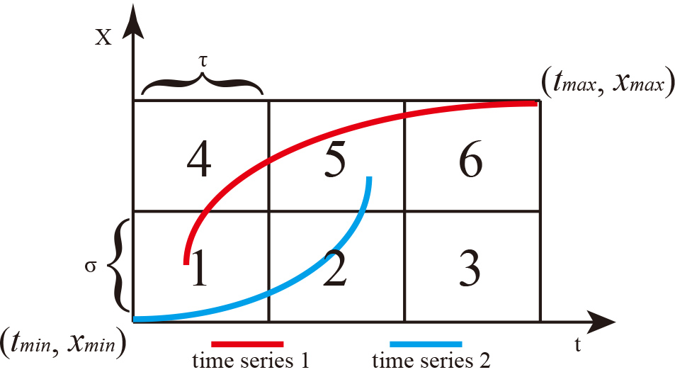

Step 2: divide the plane in $\textit{boundary}(D)$ into some cells. These cells are set to cover the plane with a size of $\sigma\times\tau$ . Each cell can be seen as a small rectangle with a height of $\sigma$ and a width of $\tau$ . $\tau$ and $\sigma$ are two parameters to tolerate time shift and value shift, respectively [9].

Step 3: assign an ID to each generated cell and calculate the maximum value of ID. Given a specific cell, we calculate the ID according to its row and column location in the grid in the following way,

$\displaystyle ID=(\textit{row}-1)\times\textit{COLUMN\_NUM}+\textit{column},$ (2)

where COLUMN_NUM is the number of columns in the grid. We also define the ROW_NUM, which is the number of rows in the grid. For example, we can see from Fig. 1 that the number of columns is 3, and the number of rows is 2. Therefore, the ID of the cell in the second column and second row of the grid is $(2-1)\times 3+2=5$ . Similarly, the ID of the cell in the first column and second row of the grid is $(2-1)\times 3+1=4$ . It is easy to know that the maximum value of ID can be computed as follows:

$\displaystyle ID_{\max}=\textit{ROW\_NUM}\times\textit{COLUMN\_NUM}$ (3)

Step 4: associate a time series $S$ with a binary code $B C$ . The length of $B C$ is $ID_{\max}$ and the initial value of each element in the $B C$ is 0. Each index in the binary code corresponds to a cell ID in the grid.

Step 5: convert a time series $S$ into the final binary code. For each point in the time series, we first calculate its row and column location in the grid and then compute the ID of the cell it is located. Obviously, for a point $(t,x)$ in $S$ , the row and column of corresponding cell are as follows:

$\displaystyle\textit{row}=\frac{x-x_{\min}}{\sigma}+1$ (4) $\displaystyle\textit{column}=\frac{t-t_{\min}}{\tau}+1$ (5)

After calculating the row and column, we use Eq. (2) to compute the ID of the cell. We finally set the value of the corresponding index in $B C$ to 1, that is,

$\displaystyle BC(ID)=1.$ (6)

We get the corresponding $B C$ for $S$ by computing the cell IDs of all points and use this binary code to represent $S$ . For example, in Fig. 1, time series 1 passes through the cells with the ID number 1, 4, 5 and 6 so it can be represented by [1, 0, 0, 1, 1, 1]. Similarly, time series 2 can be represented by [1, 1, 0, 0, 1, 0].

Algorithm 1 shows the pseudo-code of transforming a time series $S$ to the corresponding binary code $B C$ . First, COLUMN_NUM and ROW_NUM are computed (Lines 1–2). Then we calculate the $ID_{\max}$ and initialize the value of the binary code (Lines 3–4). The length of the binary code is $ID_{\max}$ . Next, the cell ID of each point in $S$ is computed (Lines 6–8), and we set the value of the corresponding index in $B C$ to 1 (Line 9). We finally return the binary code representation of $S$ . For a time series with $n$ points, the time complexity of Algorithm 1 is $O(n)$ .

TimeSeriesTranstoBinaryCode[1] $S$ : time series; $t_{\min},t_{\max},x_{\min},x_{\max}$ : $\textit{boundary}(D)$ ; $\sigma,\tau$ : parameters $B C$ : binary code representation for $S$ ; $\textit{COLUMN\_NUM}\leftarrow(t_{\max}-t_{\min})/\tau+1$ ; $\textit{ROW\_NUM}\leftarrow(x_{\max}-x_{\min})/\sigma+1$ ; $ID_{\max}\leftarrow\textit{ROW\_NUM}\times\textit{COLUMN\_NUM}$ ; $BC\leftarrow[0,0,0,\ldots,0]$ ; $\textit{point}_{i}\in S$ $\textit{row}_{i}\leftarrow(x_{i}-x_{\min})/\sigma+1$ ; $\textit{column}_{i}\leftarrow(t_{i}-t_{\min})/\tau+1$ ; $ID_{i}\leftarrow(\textit{row}_{i}-1)\times\textit{COLUMN\_NUM}+\textit{column}% _{i}$ ; $BC(ID_{i})=1$ ; $B C$ ;

The TS2BC algorithm for time series similarity search[1] $Q$ : query time series; $D$ : time series database with binary code representations; $\sigma,\tau$ : parameters res: nearest neighbor result; $\textit{res}\leftarrow\textit{null}$ ; $\min\leftarrow\infty$ ; $BC\_Q\leftarrow\textit{TimeSeriesTranstoBinaryCode}(Q)$ ; $BC\in D$ $\textit{Hamm}\leftarrow\textit{HamDis}(BC,BC\_Q)$ ; $\textit{Hamm}<\min$ $\textit{res}\leftarrow BC$ ; $\min\leftarrow\textit{Hamm}$ ; res;

3.3 The TS2BC algorithm

When time series are converted into binary codes, their similarity can be computed with the Hamming Distance. For two binary codes $B C$ and $\widehat{BC}$ , the Hamming Distance between them, denoted by $\textit{HamDis}(BC,\widehat{BC})$ , is the number of positions $i(1\leqslant i\leqslant ID_{\max})$ where $BC(i)\neq\widehat{BC}(i)$ . That is,

$\displaystyle\textit{HamDis}(BC,\widehat{BC})=\sum_{i=1}^{ID_{\max}}\delta(BC(% i),\widehat{BC(i)})$ (7)

where

$\displaystyle\delta(x,y)=\left\{\begin{array}[]{ll}0,&\text{if }x=y;\\ 1,&\text{if }x\neq y.\\ \end{array}\right.$ (8)

For two binary codes, the smaller the Hamming Distance between them, the more similar they are. We emphasize that the Hamming Distance computation is extremely fast on modern CPUs. Specifically, the Hamming Distance between two binary codes can be calculated very fast, just using simple machine instructions such as xor and popcnt [43].

In this part, we propose the TS2BC algorithm for time series similarity search. We here consider the one nearest neighbor search. As shown in Algorithm 1, it first converts query time series $Q$ into query binary code $BC\_Q$ (Line 3) and then linear scans the binary codes in time series database $D$ to find the time series that is most similar to $BC\_Q$ (Lines 4–9). $\textit{HamDis}(BC,BC\_Q)$ is a function for calculating the Hamming Distance between $B C$ and $BC\_Q$ .

The transformation cost from $Q$ to $BC\_Q$ is $O(n)$ and the Hamming Distance can be performed with reasonably low complexity. Thus, Algorithm 1 is an efficient method for time series similarity search.

4. Discussions of TS2BC

4.1 The differences between STS3 and TS2BC

Set-based Time Series Similarity Search (STS3) [9] is a novel method to measure the similarity between two time series. STS3 also divides the plane into several cells but represents a time series as a set of cells. When time series are converted into sets, their similarity can be computed with Jaccard metric. It is computed as follows:

$\displaystyle\textit{Jaccard}(S,Q)=\frac{|S\cap Q|}{|S\cup Q|}$ (9)

where $S$ and $Q$ are two sets. Contrary to the Hamming Distance, a larger value of Jaccard metric means the more similar between two time series. We refer readers to [9] to see the detailed description of the STS3.

Figure 2.

Two examples: the differences between STS3 and TS2BC (a) and the points outside the boundary (b).

Different representation methods and different similarity measures lead to different results between TS2BC and STS3. For example, in Fig. 2a, the binary code representations of query, time series 1 and time series 2 are [1, 1, 1, 0], [1, 0, 1, 1] and [1, 0, 0, 0], respectively. Obviously, the Hamming Distance between query and time series 1 is equal to the Hamming Distance between query and time series 2, both of which are 2. However for STS3, the set representations are {1, 2, 3}, {1, 3, 4} and {1}, respectively. $\textit{Jaccard}(\textit{query},\textit{time series }1)=\frac{1}{2}$ while $\textit{Jaccard}(\textit{query},\textit{time series }2)=\frac{1}{3}$ . Thus for STS3, time series 1 is more similar to the query.

For STS3, the time complexity of converting a time series with $n$ points into a set is $O(\textit{nlogn})$ with the set implemented by an order list for the convenience of linear-time intersection [9]. However, for TS2BC, the transformation cost from a time series to binary code is $O(n)$ . The Jaccard similarity computation cost of the sets is $O(|S|+|Q|)$ using a simple linear merge while the Hamming Distance between two binary codes can be calculated extremely fast just using simple machine instructions such as xor and popcnt. Therefore, theoretically, TS2BC performs faster than STS3.

4.2 Processing points outside the boundary

In the previous discussion, we assumed that all time series are limited in a $\textit{boundary}(D)$ . Since the boundary is generated by the database $D$ , points outside the boundary can only appear in the query time series. Figure 2b illustrates a concrete example. In general, most of the points in the query time series are inside the boundary. For points outside the boundary, which have no intersection with the time series in $D$ , we ignore them because taking them into account does not change the ranking of the Hamming Distance between query and time series in $D$ . With such a method, the binary code representations of query time series 1 and query time series 2 in Fig. 2b are [1, 1, 1, 0, 0, 1, 0, 0, 0] and [1, 0, 0, 1, 0, 0, 1, 1, 0], respectively.

4.3 Processing time series with missing values and noise

Time series with missing values and noise occur in many applications. Missing data and noise in practice can significantly deviate the outcomes of time series data mining, and, thus, it is crucial to treat them properly. In this part, we show that, with suitable parameters, our algorithm is not sensitive to missing data and noise, and we can eliminate the impact of them on time series.

Figure 3.

An example of processing time series with missing values and noise.

Figure 3 shows an example of the TS2BC algorithm for processing time series with missing values and noise. Figure 3a–c present the original time series, time series with Gaussian noise and time series with missing data, respectively. Given suitable parameters, their corresponding binary code representations can be found in Fig. 3d–f. Obviously, it can be seen from Fig. 3 that the three time series have the same binary code representation: [000111, 101101, 111000]. Thus, TS2BC has the ability to eliminate the effect of noise and missing data on time series. In fact, it is parameters, $\sigma$ and $\tau$ , which can tolerate value shift and time shift, that make our approach robust. And in next subsection, we will discuss the impact of the parameters.

4.4 The impact of parameters

From the TS2BC algorithm descriptions, we observe that the major factor that affects the search results is the size of cell ( $\sigma\times\tau$ ).

Figure 4.

The impact of parameters: small cell (a), appropriate cell (b) and large cell (c).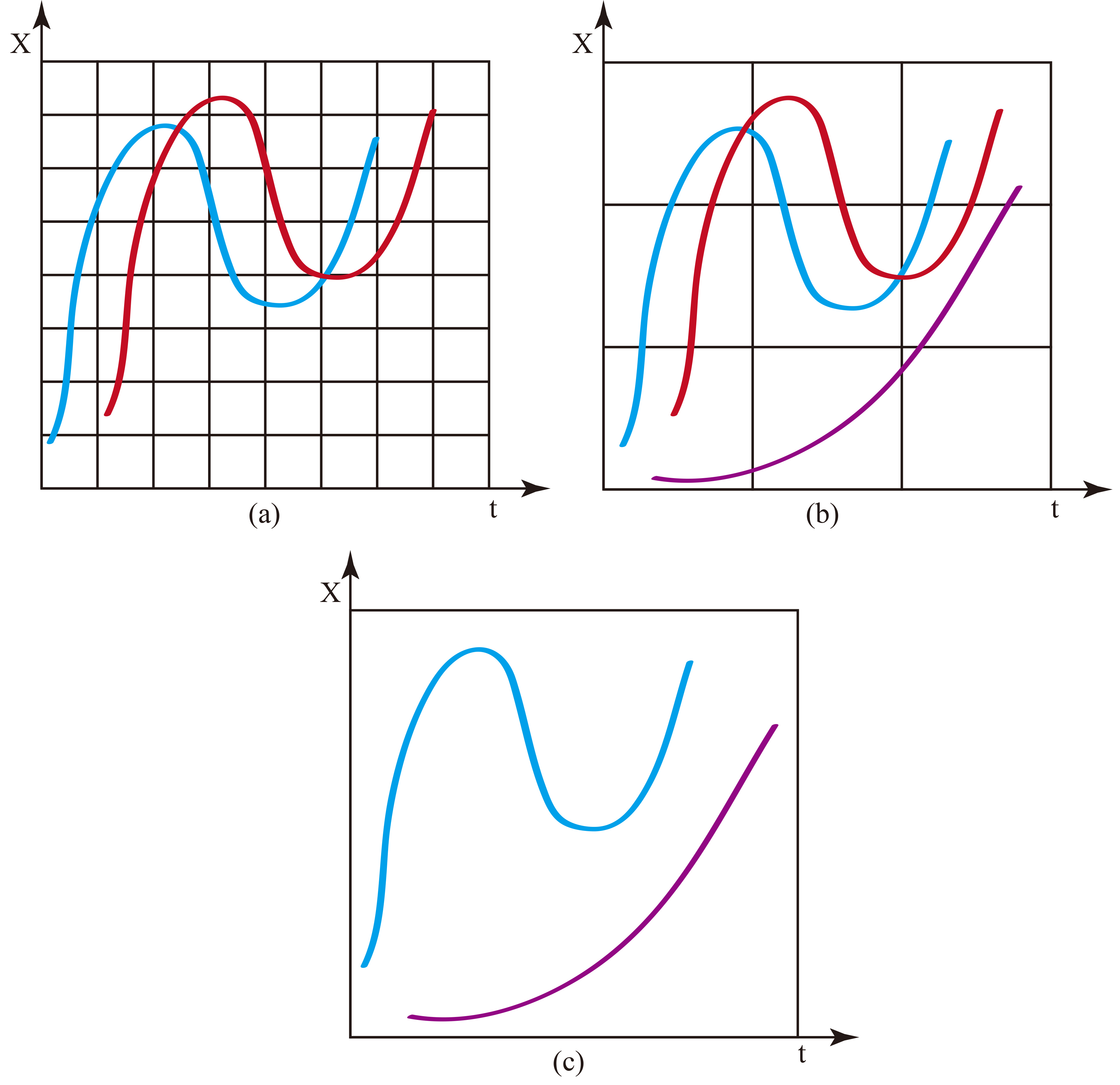

Figure 4a demonstrates that a small cell will lose the ability to handle the time shift and value shift: two shifted time series in Fig. 4a almost pass through completely different cells. Visually, anyone would confirm that the two time series in the Fig. 4a are very similar to each other, however, in our TS2BC method, these two time series are totally different. On the other hand, a large cell may cause different points to fall into the same cell and to be regarded as one point. An extreme example can be found in Fig. 4c, in which the cell has the same size as the boundary. Two completely different time series have the same binary code in Fig. 4c, which would overestimate the similarity. Thus, proper parameters can make our algorithm perform better, as shown in Fig. 4b. TS2BC can handle shifted time series and has the ability to distinguish between different classes of time series data when cells have the appropriate parameters.

Parameters are important for our method, and they need to balance the ability to hold shift and distinguish between different classes time series. We will discuss the choice of parameters in Section 6.

5. Approximate TS2BC algorithm

The value of the $ID_{\max}$ has a significant influence on the efficiency of the algorithm. Long binary codes will make TS2BC inefficient. Therefore, in this section, we propose an approximate version of TS2BC (ATS2BC) algorithm for long binary codes, which may miss the most similar time series in some cases but is much faster than TS2BC.

To facilitate concise discussions, we divide the plane into $\textit{scale}\times\textit{scale}$ cells. Obviously, the parameter scale satisfies the following equation.

$\displaystyle\frac{t_{\max}-t_{\min}}{\tau}+1=\frac{x_{\max}-x_{\min}}{\sigma}% +1=\textit{scale}.$ (10)

Figure 5.

Two time series in different scales.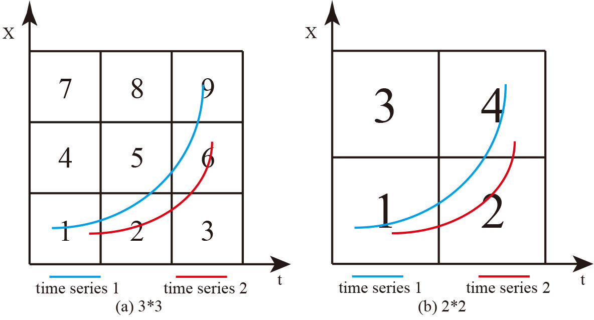

The approximate algorithm is based on the observation that if two time series are similar in a refined scale, then they are probably similar in a coarse scale [9]. We present a concrete example to illustrate this observation graphically. In Fig. 5a, when $\textit{scale}=3$ , the binary code representations of time series 1 and time series 2 are [1, 1, 0, 0, 1, 1, 0, 0, 1] and [1, 1, 1, 0, 0, 1, 0, 0, 0], respectively. The Hamming Distance between them is 3, however, in Fig. 5b, when $\textit{scale}=2$ , both of binary code representations are [1, 1, 0, 1], so the Hamming Distance is 0. Note that the smaller the value of scale, the lower the dimension of the binary codes. Therefore, the time required for the query can be reduced if a lot of similarity computations are performed in the coarse scale.

Based on this observation, we propose the ATS2BC algorithm. Given a query time series $q$ , ATS2BC first calculates the Hamming Distance from $q$ to every time series in dataset in the coarsest scale and selects candidates which have the minimal Hamming Distance to the query. Compared to other time series, candidates are more likely to be the nearest neighbor of $q$ . To further filter out more time series, ATS2BC then refines these candidates in a more refined scale. The process of refining and calculating is continued until $k$ -nearest neighbors are found, where $k$ is a threshold predefined. ATS2BC finally examines the 1-nearest neighbor by calculating the Hamming Distance in the raw scale among the remaining $k$ time series. In this way, many Hamming Distance computations can be calculated in low-dimensional space. As a result, the query processing is accelerated.

ATS2BC can be divided into offline pre-processing process and online query process. Algorithm 5 is the pre-processing process of the ATS2BC. It first divides the plane into several cells in scale from minScale to maxScale and then computes the binary code representation of each time series in each level.

Pre-processing of the ATS2BC[1] minScale, maxScale: parameters; $D$ : time series database; Scale_BC: binary code representation of each time series in each scale; $\textit{scale}=\textit{minScale}$ to maxScaleeach time series $T\in D$ $\textit{Scale\_BC}[\textit{scale}][T]$ $\leftarrow$ binary code representation of $T$ in scale division;

Scale_BC;

The procedure of ATS2BC[1] $\textit{minScale},\textit{maxScale},\sigma,\tau,\textit{threshold}$ : parameter; $D$ : time series database; $Q$ : query time series;Scale_BC: binary code representation of each time series in each scale res: approximate nearest neighbor results; candidateSet $\leftarrow$ all time series of $D$ ; $\textit{scale}=\textit{minScale}$ to maxScale ${BC\_Q}\leftarrow$ binary code representation of $Q$ in scale division; $\min\leftarrow\infty$ time series $T\in\textit{candidateSet}$ $\textit{temp}\leftarrow\textit{HamDis}(\textit{Scale\_BC}[\textit{scale}][T],% BC\_Q)$ ; $\textit{temp}<\min$ $\min\leftarrow\textit{temp}$ ; $\textit{newCandidateSet}\leftarrow\textit{null}$ ; time series $T\in\textit{candidateSet}$ $\textit{HamDis}(\textit{Scale\_BC}[\textit{scale}][T],BC\_Q)==\min$ $\textit{newCandidateSet.add}(T)$ ; $\textit{candidateSet}\leftarrow\textit{newCandidateSet}$ ; $\textit{candidateSet.size}<\textit{threshold}$ break; $\textit{res}=TS2BC(Q,\textit{candidateSet},\sigma,\tau)$ res;

The detailed online query process of ATS2BC can be found in Algorithm 5. We initialize the candidates with all time series in the database (Line 1). The binary code representation of the query time series in each scale is computed in Line 3. We calculate the minimal Hamming Distance to query in scale (Lines 4–10) and preserve all time series with the minimal Hamming Distance while removing others from candidateSet (Lines 11–17). If the size of the candidateSet is less than the specified threshold, we exit the loop (Lines 18–20). It is worth noting that the threshold should be much smaller than the size of the database. We finally call TS2BC to calculate the nearest neighbor in candidateSet (Line 22).

Although the ATS2BC can improve efficiency, only approximate nearest neighbor results can be obtained. It may miss the time series that are most similar to the query, for example, in Fig. 6a, time series 1 is most similar to the query. The Hamming Distance between query and time series 1 is 0, while it is 6 between query and time series 2. However, as Fig. 6b illustrates, when the plane is divided into a coarse scale, obviously, time series 2 is most similar to the query, both have the same binary code of [1, 1, 0, 1]. Therefore, the time series, which is most similar to the query, is missed in a coarse scale according to Algorithm 5. Fortunately, this situation is rare on the real datasets [9].

Note that the ATS2BC method described here follows the approximate STS3 (ASTS3) algorithm presented in [9]. However, ASTS3 is based on the Jaccard Metric, while ATS2BC is based on Hamming Distance. Thus, ATS2BC can take advantage of binary code. Moreover, in ASTS3, minScale and threshold are fixed to 2 and 1 respectively, however, in our method ATS2BC, minScale and threshold are two parameters, and their values will be adjusted according to different datasets. Therefore, compared with ASTS3, our algorithm has better flexibility.

Figure 6.

Example of missing the time series that are most similar to the query when using ATS2BC.

6. Experiments

To empirically evaluate the effectiveness and efficiency of the proposed methods, we conduct extensive experiments. In this section, we report and analyze the experimental results. We implemented all algorithms in MATLAB, and ran all the experiments using Windows 7 enterprise with 3.30 GHz CPU and 8GB memory.

6.1 Experimental setting

6.1.1 Datasets

We conduct our experiments on the well-known UCR archive [44], which is the primary benchmark for most time series classification studies. Detailed information on the sizes of datasets and lengths of time series can be found on the UCR website. Each dataset has two parts, TRAIN and TEST, and each time series in the dataset is labeled. As we will see, we use this split of the datasets for the similarity measure evaluation; we also use the TRAIN for tuning the parameters. Before performing the experiments, all datasets were normalized for all algorithms.

6.1.2 Experiment scheme

The proposed methods are validated by the one-nearest neighbor (1NN) classification method. Specifically, For each time series in TEST, the 1NN classifier calculates the similarity between it and all the time series in TRAIN, and its class is computed according to its nearest neighbor in TRAIN. We select the 1NN classifier as the validation method because it has several advantages [14]. First, the accuracy of the 1NN classifier directly reflects the effectiveness of the similarity measure. Second, the 1NN classifier is straightforward to implement and is parameter-free, which makes it easy for anyone to reproduce our results. Third, it has been suggested that the 1NN classifier can obtain the best results in time series classification.

Three representative approaches are selected to compare with the proposed method, including Euclidean Distance (1NN-ED), Dynamic Time Warping (1NN-DTW) and STS3. Besides, we also compare ATS2BC and TS2BC in terms of efficiency and effectiveness in this section.

6.1.3 Parameter settings

Proper parameters can make our algorithm perform better, and practically, the parameters of the TS2BC should be determined before testing.

The value of $\sigma$ and $\tau$ that we use for the similarity search are dependent on the dataset. For each dataset, all parameters should be found using the TRAIN dataset. Specifically, we randomly select half of the time series in TRAIN as the training set and the other half as the test set. Experiments for accuracy using the 1NN classification framework are conducted with various parameters $\sigma$ and $\tau$ . Due to the computation complexity, it is impossible to perform all the experiments using all parameter combinations. Therefore, we search the best parameter combination in two steps [10]. First, the value of $\sigma$ is in the range of 0.1–1 with fixed step size 0.1, and the value of $\tau$ ranges from 1 to $0.3*n$ with fixed step size 5. The parameters with the best accuracy are selected. If the best accuracy is the same for more than one parameter combination of $\sigma$ and $\tau$ , we select the pair with a minimal value of $ID_{\max}$ . Table 1 shows the parameter settings for TS2BC in the second step after a parameter combination $(\hat{\sigma},\hat{\tau})$ with best accuracy was found in the first step. As before, the parameters with the best accuracy are selected.

Table 1
Parameter settings for TS2BC in the second step

Parameter	Minimum value	Maximum value	Step size
$\sigma$	$\hat{\sigma}-0.1$	$\hat{\sigma}+0.1$	0.02
$\tau$	$\hat{\tau}-5$	$\hat{\tau}+5$	1

6.2 Comparison with STS3

We first compare our method with STS3 for two reasons.

•
Our method is inspired by the STS3 but uses different representation method and similarity measurement. We are very interested in which of these two algorithms performs better.
•
From [9], we know that STS3 is faster than most existing methods. For example, STS3 is 2905 times faster than FastDTW on CinC_ECG_torso dataset. FastDTW [45] is an optimization technique based on DTW. If experiments show TS2BC is more efficient than STS3, we can indirectly explain that our method is also faster than most existing algorithms.

Table 2
Datasets descriptions

Name #TRAIN #TEST Length ( $\sigma,\tau$ )

DistalPhalanxTW 139 400 80 (0.78, 17)

Gun_Point 50 150 150 (0.6, 4)

Coffee 28 28 286 (0.5, 4)

OliveOil 30 30 570 (0.5, 3)

Haptics 155 308 1092 (0.5, 20)

HandOutlines 370 1000 2709 (0.5, 40)

In this subsection, we mainly compare TS2BC with STS3 in terms of efficiency. Effectiveness comparisons with STS3 and other algorithms can be found in the next subsection. We use six datasets to evaluate the efficiency of TS2BC. These six datasets are selected because we want to test the impact of time series length on efficiency. The information on the datasets and the parameters for STS3 and TS2BC are described in Table 2, where #TRAIN means the total number of time series in TRAIN. Without loss of generality, in this subsection, we set the same parameters for both algorithms.
6.2.1 Pre-processing time

Name	#TRAIN	#TEST	Length	( $\sigma,\tau$ )
DistalPhalanxTW	139	400	80	(0.78, 17)
Gun_Point	50	150	150	(0.6, 4)
Coffee	28	28	286	(0.5, 4)
OliveOil	30	30	570	(0.5, 3)
Haptics	155	308	1092	(0.5, 20)
HandOutlines	370	1000	2709	(0.5, 40)

Before the query process is executed, the time series in TRAIN need to be transformed into sets or binary codes. This experiment aims to test the pre-processing time on real datasets.

We report the speedup rate, which reflects how fast an algorithm is with respect to another algorithm. Let $t_{1}$ be the pre-processing time for STS3 and $t_{2}$ be the pre-processing time for TS2BC. Then, the pre-processing time of the speedup rate of the TS2BC is $t_{1}/t_{2}$ .

Figure 7a illustrates that the pre-processing time of the TS2BC is very small compared to the STS3. TS2BC can achieve 80 to 550 times faster than STS3. Moreover, we find that the length of the time series has a significant impact on efficiency: speedup rate increases as the length of the time series increases. It is easy to understand because for STS3, the time complexity for a time series with $n$ points transformed into a set is $O(\textit{nlogn})$ , while for TS2BC, the cost is only $O(n)$ .

Figure 7.

Pre-processing time speedup rate (a) and query time speedup rate (b) of TS2BC compared to STS3 on various datasets.

Figure 8.

The relationship between $ID_{\max}$ and speedup rate.

6.2.2 Query processing time

A practical and important issue is the efficiency of the query processing time. As analyzed theoretically, in general, STS3 has a higher time complexity than TS2BC. We compare the empirical running time of two algorithms on the above 6 UCR datasets. We also report the speedup rate of TS2BC compared to STS3.

Figure 7b demonstrates the query processing time for each of the methods on various datasets. It can be seen that TS2BC performs fast than STS3 on all datasets. Specifically, TS2BC can achieve 2 to 26 times faster than STS3. In most of the situations, as the length of the time series increases, the efficiency of the TS2BC decreases. However, for the three datasets OliveOil, Haptics and HandOutlines, the situation is quite different.

We briefly explain the reasons for these situations. The Jaccard similarity computation cost of the sets is $O(|S|+|Q|)$ , where $|S|$ and $|Q|$ represent the number of elements in the set $S$ and $Q$ , respectively. In general, $|S|$ and $|Q|$ can increase when $ID_{\max}$ is added (please refer to the definition of the $ID_{\max}$ to get the idea). On the other hand, the computation cost of the Hamming Distance depends on the length of the binary code. It should be clear that the length of the binary code is equal to $ID_{\max}$ . Thus both methods of calculating similarity are independent of the time series length. As a result, time series length has no direct effect on the speedup rate while $ID_{\max}$ may have a great impact on speedup rate.

The relationship between speedup rate and $ID_{\max}$ can be found in Fig. 8, which shows that speedup rate can decrease when $ID_{\max}$ is increased. The reason may be that when $ID_{\max}$ is increased, compared with Jaccard similarity, we need to add more time to calculate Hamming Distance.

6.3 Effectiveness

We compare TS2BC with STS3 and two state-of-the-art techniques, including 1NN-ED and 1NN-DTW, to evaluate the effectiveness of TS2BC. We use 61 representative datasets in the UCR Archive and one nearest neighbor classifier to evaluate the effectiveness of the four algorithms. The error rate is reported, which is calculated as follows:

$\displaystyle\textit{errorRate}=\frac{\textit{number of wrongly classified % time series}}{\textit{total number of time series in TEST}}.$

The results for STS3, 1NN-ED and 1NN-DTW are taken directly from publications or websites of the authors. We document error rates of four algorithms in Appendix A. The lowest error rate on each dataset is highlighted in bold font.

Figure 9 represents visually the error rates of TS2BC paired with 1NN-ED, 1NN-DTW and STS3. Each axis represents a method, and each point represents the error rate for a particular dataset. The line $x=y$ is drawn to represent the region where both methods perform about the same. Points below the line indicate that TS2BC is more accurate than the other method in the pair. In general, we can find that no single method outperforms all other methods for all datasets. We observe that TS2BC clearly outperforms 1NN-ED, and the accuracy of STS3 is comparable to our method. However, 1NN-DTW exceeds TS2BC in most cases.

Figure 9.

The classification error rates of four methods. Each point represents a dataset. Points below the line mean that TS2BC is more accurate than the other method in the pair.

Figure 10.

Number of datasets in each compression ratio interval.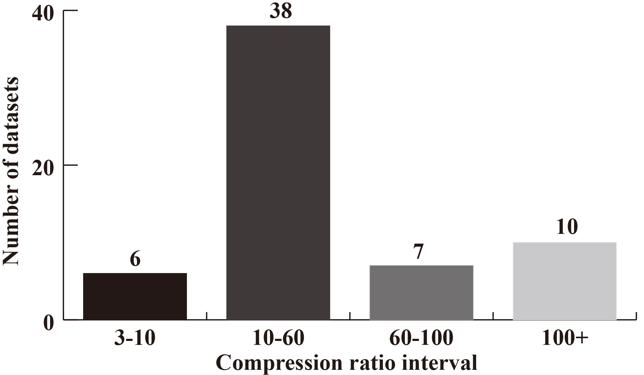

Furthermore, the average error rate of each method for all datasets is calculated. 1NN-DTW has a minimum average error rate of 0.2513. It is understandable because 1NN-DTW has been successfully used for time series similarity search and shown to be very hard to beat [33, 34, 14]. Just inferior to the 1NN-DTW, our method achieves 0.2794 for average error rate, followed by the STS3, which achieves an average error rate of 0.2883. The 1NN-ED is not stable, and its performance mainly depends on the dataset. Although it can achieve the best results in some datasets, in other datasets, its performance is not good enough, with an average error rate of 0.3001.

Overall, our proposed method TS2BC performs best on some datasets in accuracy and achieves comparative performance on remaining datasets. Moreover, TS2BC can achieve much higher efficiency than most existing algorithms in all cases. For example, it is 3596 times faster than DTW on the Coffee dataset and 939 times faster than DTW on the ECG200 dataset. Thus, TS2BC can be applied in different fields, especially in real-time applications where the responsiveness is important.

6.4 Compression ratio

As mentioned earlier, TS2BC is storage efficient. As traditional time series compression algorithms did, we define the compression ratio as the ratio between the size of the original datasets and that of the compressed one. Formally, we reasonably assume each time series value is a 32-bit float number, then the storage cost of the raw time series dataset $D$ is $32\times N\times n$ bits, where $n$ is the length of the time series and $N$ is the number of time series in $D$ .

From the TS2BC descriptions, we know that the storage cost of the proposed representation method mainly depends on one factor, $ID_{\max}$ , for a particular dataset. We use 1-bit to store each element in the binary code. Therefore, the storage cost of our representation scheme is $1\times N\times ID_{\max}$ bits. Thus, the compression ratio can be calculated as follows,

$\displaystyle\textit{Compression ratio}=\frac{32\times N\times n}{1\times N% \times ID_{\max}}=\frac{32\times n}{ID_{\max}}.$ (11)

Figure 10 shows the results of compression ratio on 61 UCR datasets. TS2BC can achieve 59.56 compression ratio on average, with a maximum compression ratio of 661 on InlineSkate datasets. This suggests that TS2BC can compactly represent the original time series.

6.5 Evaluation of the ATS2BC

We conduct this experiment to compare the efficiency and accuracy between TS2BC and ATS2BC. We use three datasets in the UCR Archive: ECG5000, Haptics, uWaveGestureLibrary_Y (UWGLY). The information on these datasets and the setting of parameters are listed in Table 3. The parameter minScale is set to 5, maxScale is set to 7 and threshold is set to $\frac{\textit{\#TRAIN}}{10}$ on all datasets, where #TRAIN means the total number of time series in TRAIN. These datasets are selected because their $ID_{\max}$ are large enough and ATS2BC is applied to the scenario when the dataset has a large value of $ID_{\max}$ .

Table 3
Datasets descriptions on three datasets

Dataset	#TRAIN	#TEST	Length	( $\sigma,\tau$ )	$ID_{\max}$
ECG5000	500	4500	140	(0.2, 5)	1400
Haptics	155	308	1092	(0.5, 20)	1595
UWGLY	896	3582	315	(0.24, 10)	1568

Figure 11.

Evaluation of ATS2BC in terms of efficiency (a) and accuracy (b).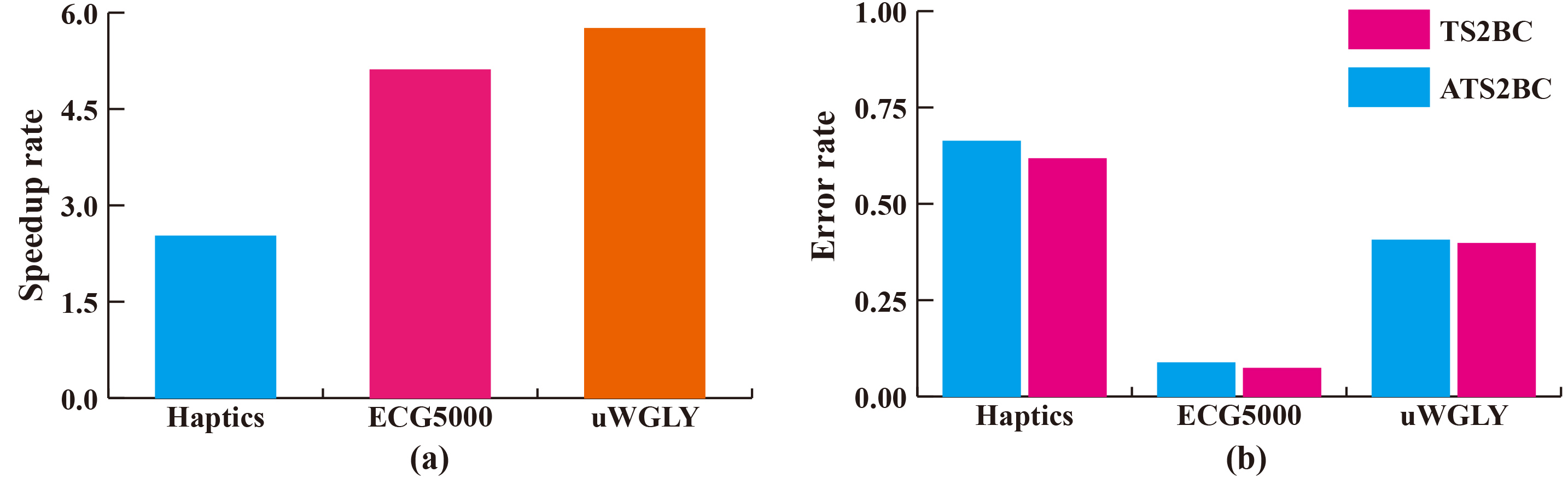

The speedup rate of ATS2BC is shown in Fig. 11a. From the results, we observe that ATS2BC is faster than TS2BC as we expected. However, as shown in Fig. 11b, the classification accuracy of the ATS2BC is only a little smaller than TS2BC. Therefore, ATS2BC is an effective method that can improve the efficiency of the TS2BC.

6.6 Case study

We provide a case study in which we applied our method to a dataset. This subsection demonstrates that TS2BC is useful and helps the reader gain an appreciation for the TS2BC.

6.6.1 DistalPhalanxTW dataset

There are 6 classes in this dataset which contains 539 time series of length 80, with 139 time series as TRAIN and other 400 as TEST. For this dataset, both ROW_NUM and COLUMN_NUM have a value of 5, and thus the $ID_{\max}$ is 25.

In our experiment, we select two different classes of time series in TEST as our queries and then use TS2BC algorithm to find their nearest neighbor in TRAIN. Figure 12 shows the results. For the convenience of our explanation, we use (a) to represent the time series in Fig. 12(a), the same for (b), (c) and (d). In this experiment, (a) and (c) are queries, and (b) and (d) are their nearest neighbor, respectively.

Table 4
Binary code representations for four time series in Fig. 12

Time series	Binary code representation
(a)	00011, 11111, 11111, 11100, 11100
(b)	00011, 11111, 11111, 11100, 11100
(c)	00000, 11011, 11110, 11100, 11100
(d)	00000, 11011, 11110, 11100, 11100

Figure 12.

A case study on DistalPhalanxTW dataset. (a) and (c) are queries, and (b) and (d) are their nearest neighbor obtained by TS2BC, respectively.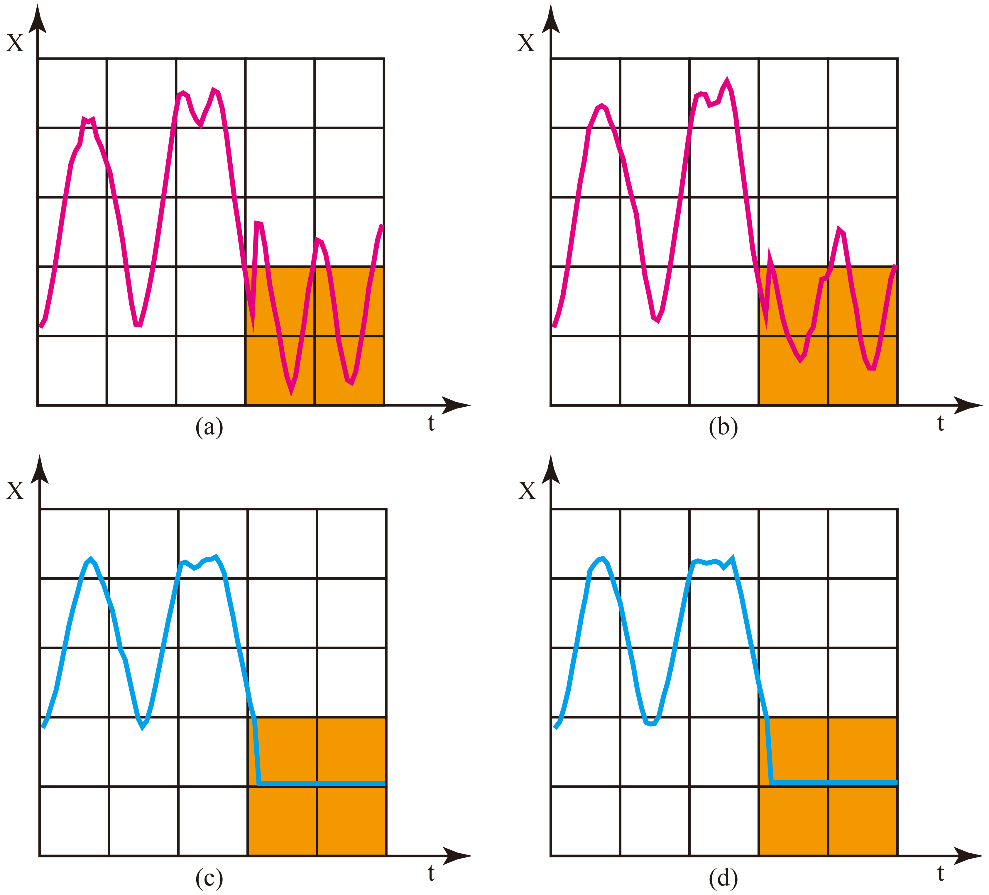

Our algorithm is based on the idea that similar time series always pass through similar cells in a plane. We use a query time series (a) as an example to illustrate the effectiveness of our algorithm. We could discover that (a) and (b) are similar, and from Table 4, we know the Hamming Distance between their corresponding binary code is 0. In fact, (a) and (b) belong to the same class and they pass through the same cells. On the other hand, for time series (a) and (d) belonging to different categories, although their first half is similar, they are quite different in the colored region, and the Hamming Distance between their binary code is 4. Therefore, under TS2BC, (d) cannot be the nearest neighbor of (a).

7. Conclusion and future work

In this paper, we propose a method, TS2BC, for processing time series similarity search problem. TS2BC uses binary code to represent time series and adopts Hamming Distance to measure the similarity between two time series. TS2BC is based on the notion that similar time series always pass through similar cells in a plane. The idea of TS2BC is consistent with human intuition. We extensively compare TS2BC with the state-of-the-art time series similarity search algorithms on 61 public datasets. Experimental results show that the accuracy of TS2BC is comparable to Dynamic Time Warping (DTW), and TS2BC can achieve much higher efficiency than most existing algorithms. Furthermore, we propose ATS2BC algorithm to speed up the query procedure and test its efficiency by experiment.

The experiment in this paper has focused on classification of the time series. It is pretty straightforward to also apply our method for clustering time series. It will be interesting to evaluate the clustering results under the Hamming Distance. Another interesting direction is applying our method for multivariate time series.

Footnotes

Acknowledgments

This work was supported by National Key Research&Development Program of China (No. 2019YFC1520905), Key Scientific Research Base for Digital Conservation of Cave Temples (Zhejiang University), State Administration for Cultural Heritage.

Appendix A: More experimental results

Table 5

Error rates of different algorithms on 61 time series datasets

Datasets	1NN-ED	1NN-DTW	STS3	TS2BC
50words	0.369	0.242	0.299	0.2857
Adiac	0.389	0.391	0.435	0.4578
ChlorineConcentration	0.35	0.35	0.395	0.4271
CinC_ECG_torso	0.103	0.07	0.063	0.07
Coffee	0	0	0.036	0.035
Computers	0.424	0.38	0.316	0.324
Cricket_X	0.423	0.228	0.308	0.3051
Cricket_Y	0.433	0.238	0.326	0.3128
Cricket_Z	0.413	0.254	0.3	0.2744
DistalPhalanxTW	0.273	0.272	0.308	0.215
Earthquakes	0.326	0.258	0.317	0.304
ECG200	0.12	0.12	0.16	0.13
ECG5000	0.075	0.075	0.075	0.073
ECGFiveDays	0.203	0.203	0.225	0.228
FaceAll	0.286	0.192	0.267	0.268
FacesUCR	0.231	0.088	0.195	0.2024
FISH	0.217	0.154	0.246	0.217
FordB	0.442	0.414	0.488	0.4543
Gun_Point	0.087	0.087	0.227	0.12
HandOutlines	0.199	0.197	0.213	0.225
Haptics	0.63	0.588	0.653	0.6169
Herring	0.484	0.469	0.438	0.469
InlineSkate	0.658	0.613	0.696	0.7145
InsectWingbeatSound	0.438	0.422	0.454	0.4333
ItalyPowerDemand	0.045	0.045	0.126	0.0544
Lighting7	0.425	0.288	0.301	0.274
MALLAT	0.086	0.086	0.135	0.1458
Meat	0.067	0.067	0.1	0.1167
MedicalImages	0.316	0.253	0.357	0.3737
MiddlePhalanxOutlineAgeGroup	0.26	0.253	0.218	0.245
MiddlePhalanxOutlineCorrect	0.247	0.318	0.327	0.2917
MiddlePhalanxTW	0.439	0.419	0.456	0.4286

Table 6

Error rates of different algorithms on 61 time series datasets: continued

Datasets	1NN-ED	1NN-DTW	STS3	TS2BC
MoteStrain	0.121	0.134	0.167	0.1789
OliveOil	0.133	0.133	0.2	0.2
PhalangesOutlinesCorrect	0.239	0.239	0.268	0.3205
Phoneme	0.891	0.773	0.873	0.8581
ProximalPhalanxOutlineAgeGroup	0.215	0.215	0.19	0.122
ProximalPhalanxOutlineCorrect	0.192	0.21	0.203	0.244
ProximalPhalanxTW	0.292	0.263	0.235	0.2775
RefrigerationDevices	0.605	0.56	0.539	0.5493
ScreenType	0.64	0.589	0.563	0.616
ShapesAll	0.248	0.198	0.225	0.2433
SmallKitChenAppliances	0.659	0.328	0.363	0.365
SonyAIBORobotSurface	0.305	0.305	0.388	0.3095
SonyAIBORobotSurfaceII	0.141	0.141	0.297	0.2403
SwedishLeaf	0.211	0.154	0.16	0.17
synthetic_control	0.12	0.017	0.05	0.0333
ToeSegmentation1	0.32	0.25	0.18	0.1711
ToeSegmentation2	0.192	0.092	0.146	0.0692
Trace	0.24	0.01	0.12	0.04
Two_Patterns	0.09	0.002	0.032	0.028
uWaveGestureLibrary_X	0.261	0.227	0.253	0.261
uWaveGestureLibrary_Y	0.338	0.301	0.323	0.397
uWaveGestureLibrary_Z	0.35	0.322	0.332	0.349
UWaveGestureLibraryAll	0.052	0.034	0.041	0.047
wafer	0.005	0.005	0.009	0.0115
Wine	0.389	0.389	0.481	0.444
WordsSynonyms	0.382	0.252	0.346	0.3621
Worms	0.635	0.586	0.558	0.5193
WormsTwoClass	0.414	0.414	0.392	0.3536
yoga	0.17	0.155	0.196	0.1743

References

Abe

Ohsaki

Yokoi

and Yamaguchi

, Implementing an integrated time-series data mining environment based on temporal pattern extraction methods: a case study of an interferon therapy risk mining for chronic hepatitis, in: Annual Conference of the Japanese Society for Artificial Intelligence, Springer, 2005, pp. 425–435.

Shasha

, Tuning time series queries in finance: case studies and recommendations, IEEE Data Eng. Bull. 22(2) (1999), 40–46.

Wang

and Sun

, Energy-aware scheduling of surveillance in wireless multimedia sensor networks, Sensors 10(4) (2010), 3100–3125.

Weigend

A.S.

, Time series prediction: forecasting the future and understanding the past, Routledge, 2018.

Liao

T.W.

, Clustering of time series data – a survey, Pattern Recognition 38(11) (2005), 1857–1874.

Song

Wang

Zhang

and Fan

, Empirical study of symbolic aggregate approximation for time series classification, Intelligent Data Analysis 21(1) (2017), 135–150.

Shokoohi-Yekta

Chen

Campana

Zakaria

and Keogh

, Discovery of meaningful rules in time series, in: Proceedings of the 21th ACM SIGKDD International Conference on Knowledge Discovery and Data Mining, ACM, 2015, pp. 1085–1094.

Nakamura

Taki

Nomiya

Seki

and Uehara

, A shape-based similarity measure for time series data with ensemble learning, Pattern Analysis and Applications 16(4) (2013), 535–548.

Peng

Wang

and Gao

, Set-based similarity search for time series, in: Proceedings of the 2016 International Conference on Management of Data, SIGMOD Conference 2016, ACM, 2016, pp. 2039–2052.

10.

Jiang

Dou

and Yang

, Similarity measures for time series data classification using grid representation and matrix distance, in: Knowledge and Information Systems, 2018, pp. 1–30.

11.

Zhang

and Pi

, A new time series representation model and corresponding similarity measure for fast and accurate similarity detection, IEEE Access 5 (2017), 24503–24519.

12.

Esling

and Agon

, Time-series data mining, ACM Computing Surveys (CSUR) 45(1) (2012), 12.

13.

Mori

Mendiburu

and Lozano

J.A.

, Similarity measure selection for clustering time series databases, IEEE Transactions on Knowledge and Data Engineering 28(1) (2015), 181–195.

14.

Wang

Mueen

Ding

Trajcevski

Scheuermann

and Keogh

, Experimental comparison of representation methods and distance measures for time series data, Data Mining and Knowledge Discovery 26(2) (2013), 275–309.

15.

Moon

and Lopez

, Skyline index for time series data, IEEE Transactions on Knowledge and Data Engineering 16(6) (2004), 669–684.

16.

Berndt

D.J.

and Clifford

, Using dynamic time warping to find patterns in time series, in: KDD Workshop, Vol. 10, no. 16, Seattle, WA, 1994, pp. 359–370.

17.

Nguyen

T.S.

and Duong

T.A.

, Time series similarity search based on middle points and clipping, in: 2011 3rd Conference on Data Mining and Optimization (DMO), IEEE, 2011, pp. 13–19.

18.

Norouzi

Punjani

and Fleet

D.J.

, Fast exact search in hamming space with multi-index hashing, IEEE Transactions on Pattern Analysis and Machine Intelligence 36(6) (2013), 1107–1119.

19.

Torralba

Fergus

and Weiss

, Small codes and large image databases for recognition, in: 2008 IEEE Conference on Computer Vision and Pattern Recognition, 2008, pp. 1–8.

20.

Zhang

Yang

Jin

Cai

and He

, A unified approximate nearest neighbor search scheme by combining data structure and hashing, in: Twenty-Third International Joint Conference on Artificial Intelligence, 2013.

21.

Keogh

Chakrabarti

Pazzani

and Mehrotra

, Dimensionality reduction for fast similarity search in large time series databases, Knowledge and information Systems 3(3) (2001), 263–286.

22.

Keogh

Chakrabarti

Pazzani

and Mehrotra

, Locally adaptive dimensionality reduction for indexing large time series databases, in: Proceedings of the 2001 ACM SIGMOD International Conference on Management of Data, Vol. 30, no. 2, 2001, pp. 151–162.

23.

Keogh

E.J.

and Pazzani

M.J.

, An enhanced representation of time series which allows fast and accurate classification, clustering and relevance feedback, in: Kdd, Vol. 98, 1998, pp. 239–243.

24.

Chen

Lian

Liu

and Yu

J.X.

, Indexable pla for efficient similarity search, in: Proceedings of the 33rd International Conference on Very Large Data Bases, VLDB Endowment, 2007, pp. 435–446.

25.

Palpanas

Vlachos

Keogh

Gunopulos

and Truppel

, Online amnesic approximation of streaming time series, in: Proceedings. 20th International Conference on Data Engineering, IEEE, 2004, pp. 339–349.

26.

Lin

Keogh

Lonardi

and Chiu

, A symbolic representation of time series, with implications for streaming algorithms, in: Proceedings of the 8th ACM SIGMOD Workshop on Research Issues in Data Mining and Knowledge Discovery, ACM, 2003, pp. 2–11.

27.

Shieh

and Keogh

, i sax: indexing and mining terabyte sized time series, in: Proceedings of the 14th ACM SIGKDD International Conference on Knowledge Discovery and Data Mining, ACM, 2008, pp. 623–631.

28.

Ratanamahatana

Keogh

Bagnall

A.J.

and Lonardi

, A novel bit level time series representation with implication of similarity search and clustering, in: Pacific-Asia Conference on Knowledge Discovery and Data Mining, Springer, 2005, pp. 771–777.

29.

Agrawal

Faloutsos

and Swami

, Efficient similarity search in sequence databases, in: International Conference on Foundations of Data Organization and Algorithms, Springer, 1993, pp. 69–84.

30.

Faloutsos

Ranganathan

and Manolopoulos

, Fast subsequence matching in time-series databases, ACM, 1994, Vol. 23, no. 2.

31.

Struzik

Z.R.

and Siebes

, Wavelet transform in similarity paradigm, in: Pacific-Asia Conference on Knowledge Discovery and Data Mining, Springer, 1998, pp. 295–309.

32.

Cai

and Ng

, Indexing spatio-temporal trajectories with chebyshev polynomials, in: Proceedings of the 2004 ACM SIGMOD International Conference on Management of Data, ACM, 2004, pp. 599–610.

33.

Batista

G.E.

Wang

and Keogh

E.J.

, A complexity-invariant distance measure for time series, in: Proceedings of the 2011 SIAM International Conference on Data Mining, SIAM, 2011, pp. 699–710.

34.

Ding

Trajcevski

Scheuermann

Wang

and Keogh

, Querying and mining of time series data: experimental comparison of representations and distance measures, Proceedings of the VLDB Endowment 1(2) (2008), 1542–1552.

35.

Jeong

Y.-S.

Jeong

M.K.

and Omitaomu

O.A.

, Weighted dynamic time warping for time series classification, Pattern Recognition 44(9) (2011), 2231–2240.

36.

Zhao

and Itti

, Shapedtw: shape dynamic time warping, Pattern Recognition 74 (2018), 171–184.

37.

Yuan

Lin

Zhang

and Wang

, Locally slope-based dynamic time warping for time series classification, in: Proceedings of the 28th ACM International Conference on Information and Knowledge Management, 2019, pp. 1713–1722.

38.

Keogh

E.J.

and Pazzani

M.J.

, Derivative dynamic time warping, in: First SIAM International Conference on Data Mining, 2001.

39.

Vlachos

Gunopoulos

and Kollios

, Discovering similar multidimensional trajectories, in: icde, IEEE, 2002, p. 0673.

40.

Chen

and Ng

, On the marriage of lp-norms and edit distance, in: Proceedings of the Thirtieth International Conference on Very Large Data Bases-Volume 30, VLDB Endowment, 2004, pp. 792–803.

41.

Chen

Özsu

M.T.

and Oria

, Robust and fast similarity search for moving object trajectories, in: Proceedings of the 2005 ACM SIGMOD International Conference on Management of Data, ACM, 2005, pp. 491–502.

42.

Rakthanmanon

Campana

Mueen

Batista

Westover

Zhu

Zakaria

and Keogh

, Searching and mining trillions of time series subsequences under dynamic time warping, in: Proceedings of the 18th ACM SIGKDD International Conference on Knowledge Discovery and Data Mining, ACM, 2012, pp. 262–270.

43.

Jegou

Douze

and Schmid

, Product quantization for nearest neighbor search, IEEE Transactions on Pattern Analysis and Machine Intelligence 33(1) (2010), 117–128.

44.

Chen

Keogh

Begum

Bagnall

Mueen

and Batista

, The ucr time series classification archive, July 2015, www.cs.ucr.edu/∼eamonn/time_series_data/.

45.

Salvador

and Chan

, Toward accurate dynamic time warping in linear time and space, Intelligent Data Analysis 11(5) (2007), 561–580.

An efficient method for time series similarity search using binary code representation and hamming distance

Abstract

Keywords

1. Introduction

2.1 Time series representations

2.2 Time series similarity measures

3. Approach: TS2BC

3.1 Background and overview

4.1 The differences between STS3 and TS2BC

4.3 Processing time series with missing values and noise

6.1 Experimental setting

6.1.1 Datasets

6.1.2 Experiment scheme

6.1.3 Parameter settings

Table 1 Parameter settings for TS2BC in the second step

6.3 Effectiveness

Table 3 Datasets descriptions on three datasets

6.6.1 DistalPhalanxTW dataset

Table 4 Binary code representations for four time series in Fig. 12

Footnotes

Acknowledgments

Appendix A: More experimental results

References

Table 1
Parameter settings for TS2BC in the second step

Table 3
Datasets descriptions on three datasets

Table 4
Binary code representations for four time series in Fig. 12