Reinforcement learning based metric filtering for evolutionary distance metric learning

Abstract

Data collection plays an important role in business agility; data can prove valuable and provide insights for important features. However, conventional data collection methods can be costly and time-consuming. This paper proposes a hybrid system R-EDML that combines a sequential feature selection performed by Reinforcement Learning (RL) with the evolutionary feature prioritization of Evolutionary Distance Metric Learning (EDML) in a clustering process. The goal is to reduce the features while maintaining or increasing the accuracy leading to less time complexity and future data collection time and cost reduction. In this method, features represented by the diagonal elements of EDML matrices are prioritized using a differential evolution algorithm. Further, a selection control strategy using RL is learned by sequentially inserting and evaluating the prioritized elements. The outcome offers the best accuracy R-EDML matrix with the least number of elements. Diagonal R-EDML focusing on the diagonal elements is compared with EDML and conventional feature selection. Full Matrix R-EDML focusing on the diagonal and non-diagonal elements is tested and compared with Information-Theoretic Metric Learning. Moreover, R-EDML policy is tested for each EDML generation and across all generations. Results show a significant decrease in the number of features while maintaining or increasing accuracy.

Keywords

Clustering distance metric learning feature selection reinforcement learning

1. Introduction

In the last few years, a massive amount of data is created daily; however, the continuous growth of these data presents a challenge in the IT world regarding the ways to determine the important portions and select from such large volume of data in an efficient and timely manner.

From the economic point of view, many organizations are unable to cope with the amount of data present in their warehouses and external data not in their possession. Because of the overload problem associated with these data, a way to provide insights on the important features of the data are vital for business agility.

To overcome the problems associated with data processing, machine learning and data mining algorithms aim to process data and extract valuable information. However, these tools may be inefficient for the ever-growing amount of data over the last few decades. Furthermore, data collection can also be time consuming and expensive. For example, medical data collected using Magnetic Resonance Imaging or sensory input data collected through the Global Positioning System can be expensive and time consuming to process. That is why data processing algorithms can offer insights on which portions of data is important which helps reduce the amount of data needed and the data collection cost.

Data processing algorithms in machine learning like clustering algorithms [6] make sense of data by grouping similar objects using their features. Another example of data processing algorithms, such as Distance Metric Learning (DML) algorithms [10], can improve the clustering quality. DML increases the clustering accuracy by learning a distance function over objects and uses a distance transformation matrix M (in case of Mahalanobis distance-based metric learning) for input space transformation where the diagonal elements represent scaling factors applied on corresponding features.

Evolutionary Distance Metric Learning (EDML) [17] is a DML algorithm that optimizes the Mahalanobis-based transformation matrix M using Evolutionary Algorithms (EA). However, EDML particularly struggles to solve high dimensional problems. Furthermore, EDML needs to optimize the elements in the matrix simultaneously, for which it requires access to all the features, including the unimportant ones in the transformation process. Additionally, EDML fails to filter or select features; instead, it uses a technique of including weights as a scaling factor to prioritize features. Thus, metric filtering and selecting the right features in EDML is crucial because wrong features may be cost-ineffective and can produce worse results.

Feature selection [20, 12], which removes useless features from the original feature set, can alleviate the EDML high dimensionality problems as it can reduce the EDML search space and complexity. However, conventional feature selection processes are unsuitable because they assume free access to the data set as a whole and select a specific subset of features for any input regardless of the behavior of DML on them.

For that purpose, sequential feature selection with Reinforcement Learning (RL) [22] is introduced. RL is a machine learning technique that maps situations to actions and adapts according to its environment behavior. RL-based feature selection can learn different subsets of features according to the input and can explicitly select and learn the important elements in a sequential manner based on performances.

In this work, we propose an alternate hybrid optimization framework in the DML field called R-EDML that combines EDML and RL-based feature selection, in which RL learns how to add features sequentially based on the accuracy resulted from DML. This hybrid system can take advantage of the evolutionary feature weighting process and the optimization of distance transformation matrix M in EDML along with the RL sequential decision making that directs attention to important portions of the input space. Moreover, the hybrid system enables R-EDML to reach better solutions and achieves promising results by dramatically reducing the feature space while increasing or maintaining accuracy. This helps to reduce the time complexity and cost of future data collection.

The rest of the paper is structured as follows: Section 2 reviews briefly the literature of conventional feature selection and RL-based feature selection. Section 3 discusses the EDML. Section 4 describes the RL. Section 5 describes the methodology along with the modeling of the RL selection control strategy. In Section 6, different testing approaches and scenarios are explained in addition to the experimental results where the hybrid system performance is tested on the UC Irvine (UCI) Machine Learning database [5]. Finally, Section 7 concludes the paper.

2. Related work

2.1 Conventional feature selection

Feature selection methods are categorized into three main classes: Filter, Wrapper, and Embedded [12]: Filter methods use variable ranking approach for variable selection, which depends on general features like variable correlation for prediction or classification. Filter methods are time-efficient; however, they sometimes select the same variables by ignoring variable relationships. The Wrapper methods keep the relations between variables, by choosing a subset of variables instead of an individual variable; this facilitates the detection of possible relations between these variables. However, they are time inefficient and suffer from the risk of overfitting if the number of observations is low. When a greedy search is used, they fail to obtain optimal solutions. Embedded methods are a combination of the previous methods; thus, they take advantage of the Filter method variable selection, feature selection, and classification tasks simultaneously.

Regularization [1] is another effective approach in feature selection; for example, $L_{1}$ regularization is based on the $L_{1}$ norm as it can drive many parameters to zero and can avoid overfitting by reducing the model complexity.

2.2 RL-based feature selection

Conversely, RL has been successful when applied to feature selection. RL is chosen because of its ability to learn the important parts of data, useful for high dimensional data sets. RL simplifies the problem by proposing a reward maximization. The RL main applications in feature selection are discussed below:

Norouzi et al. [7] suggested an RL-based attention control strategy for image recognition, in which a sequential block-based approach was used to increase the correct classification rate of partially occluded faces. In this approach, the faces were partitioned into blocks and their importance in the classification task was learned by an RL agent who learned the exact number and order of blocks needed for correct classification. This approach could reduce the number of features needed for image recognition especially if the image was incomplete or impartial.

Dulac-Arnold et al. [11] proposed an approach that used policy iteration approximation in classification, where the policy was redefined at each step until it converged. These authors converted the classification into a sequential process where RL selected the features and classified the input into one of the available classes. In that way, classification and feature selection was done by a single component.

Rückstieß [25] suggested RL-based sequential online feature selection in supervised learning domains to convert classification into a sequential decision process. The approach helped to select the next feature depending on the previously-selected features and on the performance of the classifier. The approach fed features in a sequential manner to the classifier until a correct classification was achieved.

Nguyen et al. [24] introduced an online learning algorithm using sparse coding for feature selection in high-dimensional spaces and applied it to simulated and real robotics domains. They created a different MDP formulation that incorporates a principled way to factorize the state space in a compact way, while capturing the comprehensive transition and reward dynamics information. In their work, they separated the state-attributes that define the state from the informative state-features and applied feature selection on a large number of state features to capture the transition dynamics, while maintaining a compact state space.

Hachiya et al. [13] proposed a new framework that used filter-type feature selection for RL. They used the conditional mutual information as feature selection to evaluate the independence between return and state-feature sequences. The conditional mutual information was approximated by a least-squares method.

Nezhad et al. [21] proposed a feature selection method based on deep architecture and applied it to a specific medical problem to decrease the risk of heart disease. They used individual clinical data with many features and stacked auto-encoders for feature representation in higher-level abstraction. This approach applied deep learning to identify personalized features in order to control and predict the amount of left ventricular mass indexed (LVMI). This could help identify significant risk factors affecting LVMI to body surface area.

Janisch et al. [16] tackled the problem where feature collection is costly with the goal to optimize a trade-off between the expected classification error and the feature cost. They defined the problem as a sequential decision-making problem and used Deep Q-learning where individual actions are either requesting the feature values or terminating the episode by providing a classification decision. They used neural networks for value function approximations and showed that their approach outperformed the most recent methods specifically designed for the costly features classification.

These examples use an RL-based feature selection to take advantage of RL sequential decisions in the classification process. In this study, however, we use an RL feature selection to solve the metric filtering problem by combining RL with an EDML technique in a clustering algorithm. The approach not only reduces the features but also selects the correct number of features along with specific scaling factors determined by the EDML EA for each of the selected features in the transformation metric.

3. EDML

Various DML methods, such as the nearest neighbor classification method [19] and clustering techniques [8, 23], aim to improve the clustering and classification accuracy by learning a distance metric from a data set. DML is divided into two learning techniques [10]:

1.
Unsupervised DML: This can achieve dimensionality reduction as it identifies geometric relationships in the Euclidean data space. Additionally, it can convert the input space into a low dimensional space. Simultaneously, it can avoid losing data point relationships.
2.
Semi-supervised DML: This uses auxiliary information like class labels and pairwise constraints of must-links and cannot-links in its learning. It aims to optimize a common metric transformation function by preserving similar classes and separating different classes.

EDML [17] is a semi-supervised DML technique that uses an EA to optimize its distance matrices. EDML relies on a clustering index with neighbor relation to evaluate inter- and intra-clusters and to optimize a distance transform matrix based on the Mahalanobis distance defined as:

$\displaystyle d^{2}_{i,j}=(\bm{x_{i}}-\bm{x_{j}})^{t}\textit{{M}}(\bm{x_{i}}-% \bm{x_{j}})$ (1)

where $\bm{x_{i}}=(x_{i,1},\ldots,x_{i,v})^{t}$ is the $i^{\text{th}}$ data point that has $v$ -dimensional feature vector, and M is a $v\times v$ symmetric matrix. In EDML, matrix M is the variable to be optimized. This M comprises diagonal elements that represent the actual dimensions scaling factors and non-diagonal elements that represent the correlation between different dimensions. The M optimization is conducted using self-adaptive differential evolution (jDE) algorithm [14]. This is summarized as follows:

1.
jDE creates the first generation of candidates which are the distance transformation matrices.
2.
The input space is transformed using Mahalanobis distance in Eq. (1).
3.
The cluster structure is created by any clustering technique.
4.
The clusters are evaluated with class labels and pairwise constraints using the clustering index like pairwise F-measure [18] described in Section 5.
5.
The evaluation result is sent back to jDE as the fitness for these candidates.
6.
According to the fitness, jDE selects the individuals for the next generation using a probability-based mutation and cross over and creates the next generation.
7.
This cycle is repeated until the termination condition is satisfied, and the result shows the matrix with the best performance among all its peers in all generations. Figure 1 describes this cycle.

Figure 1.
EDML life cycle.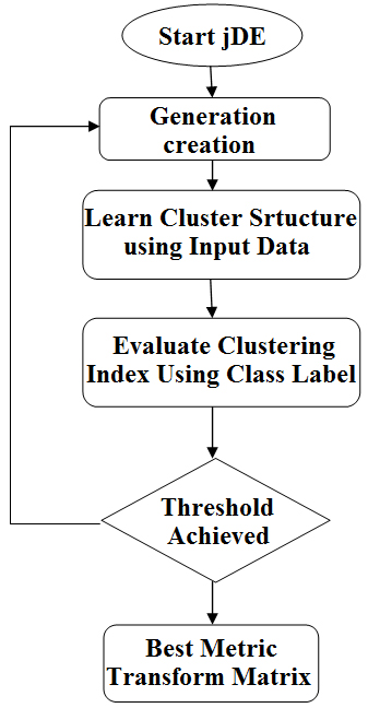

4. RL

RL [22] is a learning technique that focuses on the interaction between an agent and the surrounding world. RL enhances the agent’s behavior over time by learning from trials and errors. The agent produces an output that represents an action of the state of the world the agent is in. The state here represents the virtual representation of the world at a specific time. Moreover, the world interacts with the agent’s actions by giving a scalar value called a reward, informing the agent in this state how well its action is. The goal of the agent is to maximize the expected discounted cumulative reward.

4.1 RL overview

One of the strongest points of RL is that a model of the environment is unnecessary. Through the agent’s life span, the agent can learn a policy to follow through an interaction and a reward system. The policy defines the agent’s behavior at any given state. This is a function that maps any state of the environment with an action to be performed by the RL agent. RL algorithms are divided into two types using the agent’s information:

1.
Model-based: where the agent creates a model of the environment and finds the optimal policy by performing a planning algorithm on the model.
2.
Model-free: where the agent does not know the model of the environment. Regardless, the agent learns a policy by trial and error through a series of interactions with the environment.

An episode is a sequence of interactions between the agent and the environment from the start state to the terminal state. The agent chooses an action using the policy derived from the value function, performs this action, and observes the reward of the environment. Afterward, the agent updates its estimate of the value function associated with the policy. Then, the optimal policy is inferred by choosing the highest state-action value.
4.2 Q-learning

Q-learning is a model-free RL technique that aims to maximize a value function Q. In Q-learning, the optimal policy is derived from the highest Q-value in the current state. This is carried out by iteratively updating the Q-value function.

This process is done to optimize the Q-value function and to reach the optimal policy, described by the following equation:

$\displaystyle Q(s,a)\leftarrow Q(s,a)+\alpha[r+\gamma\max_{a^{\prime}}Q(s^{% \prime},a^{\prime})-Q(s,a)]$ (2)

where $s$ represents the state; $a$ represents the action in state $s$ ; $r$ represents the reward after taking an action in a state; $\gamma(0\leqslant\gamma<1)$ represents the discount factor, which determines how the sum of discounted rewards is calculated. Since future rewards are worth less than immediate rewards, the discount factor controls how future rewards are less than the immediate rewards. Finally, $\alpha(0<\alpha\leqslant 1)$ represents the learning rate, which controls the learning speed by controlling how the Q-values are updated. The low value refers to a slow update, which refers to slow learning, whereas the high value shows that learning can occur quickly.

5. R-EDML system architecture

The goal of this study is to minimize the used elements (features) in M in Eq. (1) while maintaining or enhancing the clustering accuracy as much as possible. K-means is the clustering algorithm used in this study using a K-nearest neighbor graph of cluster centroids. Since the EA in EDML constantly mutates and changes the elements in the distance matrices for every generation, the approach is to merge the RL sequential decision process in the EDML evolutionary generation process, taking place by inserting the elements in a sequential manner in the matrices and by learning the correct number of elements for any given EDML generation. This helps to learn the best features that suit the matrices for every generation. RL-based feature selection is suitable for EDML because RL can learn a selection control strategy, unrequired for a model of the environment, tailored to each EDML generation.

In this study, we focus on two types of EDML matrices: One is diagonal EDML where R-EDML will select from only the diagonal elements as they represent the features. The second is the Full Matrix EDML where R-EDML selects from both diagonal and non-diagonal elements to use the full power of EDML matrices transformations. Since RL is based on Markov Decision Processes (MDP), R-EDML as an MDP model is introduced; then, the life cycle of this model is described.

5.1 R-EDML model as an MDP

RL is based on MDP processes characterized by the Markov property. In MDP, every Markov state captures all the relevant information from history and independently describes the sequence of states leading to this state in the environment. The following concepts are discussed to enhance a greater understanding of the R-EDML Model as an RL model based on MDP:

1.
States
2.
Actions
3.
State transition function
4.
Reward function
5.
Terminal function

As for R-EDML, the following concepts are described:

1.
Satisfactory condition
2.
Policy

The states definition ( ${s}$ ) is the EDML transformation matrices that contain specific indices, which are the selected elements of this state.

The actions definition ( ${a}$ ) is selecting an element and inserting it into the transformation matrices. In this process, an already selected element cannot be selected again in the same episode based on the memory of the environment.

The state transition function definition [ $T(s,a,s^{\prime})$ ] is described as follows: from a state $s$ with certain elements in the matrices, the agent will take an action ${a}$ by selecting an unselected element; then, this element is inserted in the generation’s matrices and a new state $s^{\prime}$ is created and evaluated according to the newly inserted element.

The reward function [ $R(s,a)$ ] is described as follows: For every action, a negative reward of $-$ 1 called action punishment ( $A P$ ) is given to the agent; this influences the agent’s behavior to use as few elements as possible while having good accuracy. A positive reward of $+$ 10 called threshold reward ( $T R$ ) is given to the agent if the satisfactory condition is met and this terminates the episode. The total reward after an episode finishes is described as:

$\displaystyle R_{\textit{total}}=E_{\textit{selected}}\times AP+TR$ (3)

where $E_{\textit{selected}}$ is the number of the selected elements after the episode is finished. While the episode is running, given the satisfactory condition as $\theta$ , a set of selected elements is denoted as $B$ and the currently selected element after the $t^{\text{th}}$ generations of EDML is denoted as $m^{t}$ ; the value assignments of $A P$ and $T R$ are described as:

$\displaystyle TR=\left\{\begin{array}[]{ll}10,&\text{if }\theta\text{ is % satisfied}\\ 0,&\text{otherwise}\\ \end{array}\right.$ $\displaystyle AP=\left\{\begin{array}[]{ll}0,&\text{if }m^{t}\in B\\ -1,&\text{otherwise}\\ \end{array}\right.$

The terminal function is described as follows: The episode in R-EDML is terminated if the satisfactory condition ( $\theta$ ) is met or if all the elements in the matrix are selected.

The satisfactory condition ( $\theta$ ) is the criteria by which the reward and terminal functions judge how good or bad a certain state is and it focuses on reducing the number of features while obtaining an accuracy close to the EDML accuracy up to a certain range. Given the F-measure after performing an action as $F_{1a}$ , the condition is satisfied if these conditions are met:

1.
The F-measure ( $F_{1a}$ ) is close to a fixed margin $\phi$ as compared with the best EDML accuracy $[(F_{1a}-\textit{Best Accuracy})\geqslant-\phi]$ . This ensures that $F_{1a}$ can have any value higher than the best EDML accuracy but limits the best EDML accuracy when it is higher than $F_{1a}$ . This means the Best Accuracy will not exceed $\phi$ if it is higher than $F_{1a}$ , whereas $F_{1a}$ will exceed $\phi$ if is higher than the Best accuracy.
2.
The number of elements of $F_{1a}$ is equal to or less than the fewest elements recorded to achieve the best accuracy.

After both conditions are met, the values of the current best EDML accuracy and the fewest elements recorded are updated according to $F_{1a}$ to improve the agent performance by imposing a harder goal in the next phases. The comparison in the satisfactory condition shows our acceptance of the slight degradation as well as the improvement of evaluation score within the accepted margin as long as the number of features is reduced.

The policy ( $\Pi$ ), is applied in two ways:

1.
The agent learns a new policy for each generation (policy separation) based on the assumption that EDML EA mutates and changes the elements’ values after each generation, so a new policy tailored for each generation is tested.
2.
A unified policy across all generations is used that is continuously updated for all generations (policy unification).

The policy used in this research is an Epsilon greedy policy, which allows the agent to be greedy with respect to rewards with a probability of $1-\epsilon$ and also lets the agent explore as well with a probability of $\epsilon$ . This greedy exploration method is adopted because it is believed that an optimal solution is not guaranteed if the number of features is large. Given state $s$ , action $a$ , $A(s)$ as the set of available actions in s where $a\in A(s)$ and $A^{}$ as the action with the highest value function where $A^{}\leftarrow\text{argmax}_{a}Q(s,a)$ . Epsilon greedy policy $\Pi$ can be described as follows:

$\displaystyle\Pi(a|s)=\left\{\begin{array}[]{ll}1-\epsilon+\epsilon/|A(s)|,&% \text{if }a=A^{}\\ \epsilon/|A(s)|,&\text{if }a\neq A^{}\\ \end{array}\right.$
5.2 R-EDML life cycle

The overall R-EDML life cycle is divided into two phases: The EDML phase and the RL phase that run after each other in a loop for a specific number of generations. The EDML phase prepares the generation for the RL phase, whereas the RL phase gives feedback to the EDML phase to create the new generation. The detailed steps are as follows:

1.
EDML phase:

EDML evaluates the candidates using the K-means clustering algorithm and selects the elite results for the new generation using an EA. This generation’s population is a set of distance matrices M’s responsible for the data set transformation (The diagonal elements of M’s correspond to the features in the data set, whereas non-diagonal elements correspond to the correlation between different features).
2.
RL phase:

(a)
Elements of each M are stored for future reference. In the case of Diagonal R-EDML, the diagonal elements for each M are stored. In the case of Full Matrix R-EDML, both the diagonal and non-diagonal elements are stored.
(b)
All the elements in the matrices for this generation are reset to zero.
(c)
Several episodes will start, in each episode, the RL agent will insert the stored original elements in a sequential manner into the matrices M’s of the generation (each insertion is done to multiple matrices at once) and evaluate with each insertion the clustering accuracy.
(d)
Based on this evaluation, the agent either stops or continues to insert new elements (back to (c)). The termination of each episode depends on either achieving the satisfactory condition after evaluation or inserting all the elements.
(e)
After all the episodes finish, RL will use the learned policy to identify the elements that offer the best performance in this generation.
(f)
The selected features will either be saved for later comparisons or will be fed back to EDML and used in creating the next generation.
(g)
The feedback (important features learned) from the RL phase to the EDML phase is constructed in two ways: Change EDML and No Change EDML.

i.
Change EDML: the current generation is changed before being passed to the EA, this change is:

A.
Resetting the non selected elements to zero or decreasing their value by a certain fixed ratio.
B.
Setting the selected elements to their original values.

ii.
No Change EDML: the result is not fed to EDML, and all the elements are returned to their original values. EA will continue independently from RL.

EDML phase will create a new generation and RL will start learning for the new generation. The entire process continues until a fixed number of generations are created. The output is the selection of the best M that has the closest accuracy to EDML and the least number of elements possible.

As for the evaluation process, the evaluation measure used is the F-measure ( $F_{1}$ score) which is the harmonic average of recall and precision where precision is the measure of the same class among each cluster, whereas recall is the measure of the same cluster among each class. However, normal F-measure cannot be computed because there is no definite matching between cluster and class. For that reason, the F-measure used here is the pairwise F-measure [18] which is similar to normal F-measure but is evaluated in a pairwise manner on the clustering result. Pairwise manner evaluation borrows the idea of precision and recall to evaluate the clustering result and is more suitable to evaluate this problem. There are other performance measures like Purity, and Entropy [9]. Purity is the average of the ratio that a majority class occupies in each cluster while Entropy indicates the degree of unevenness of class distribution within a cluster. These measures will be used in future work.

Given $C(\bm{x_{i}})$ as the cluster index of $\bm{x_{i}}$ ; $C(\bm{x_{j}})$ as the cluster index of $\bm{x_{j}}$ ; $T(\bm{x_{i}})$ as the class index of $\bm{x_{i}}$ and $T(\bm{x_{j}})$ as the class index of $\bm{x_{j}}$ , the class and cluster confusion matrix of data pairs is defined in Table 1.

Table 1
Class and cluster confusion matrix of data pairs

$T(\bm{x_{i}})=T(\bm{x_{j}})$ $T(\bm{x_{i}})\neq T(\bm{x_{j}})$

$C(\bm{x_{i}})=C(\bm{x_{j}})$ a b

$C(\bm{x_{i}})\neq C(\bm{x_{j}})$ c d

The precision $P$ , recall $R$ and F-measure $F_{1}$ are defined as follows:

$\displaystyle P=\frac{a}{a+b}$ (4) $\displaystyle R=\frac{a}{a+c}$ (5) $\displaystyle F_{1}=2\cdot\frac{P\cdot R}{P+R}$ (6)

which ensures an incremental behavior in the performance with every generation having better accuracy or at least equal to the generation before. This gives RL an incentive to keep updating its goal and to keep up with the incremental accuracy. Figure 3 shows an example of Diagonal R-EDML system architecture with each generation having a population of 3 matrices and 3 diagonal elements (features), whereas Fig. 2 shows the R-EDML RL phase pseudo-code.

Figure 2.
R-EDML RL phase pseudo-code.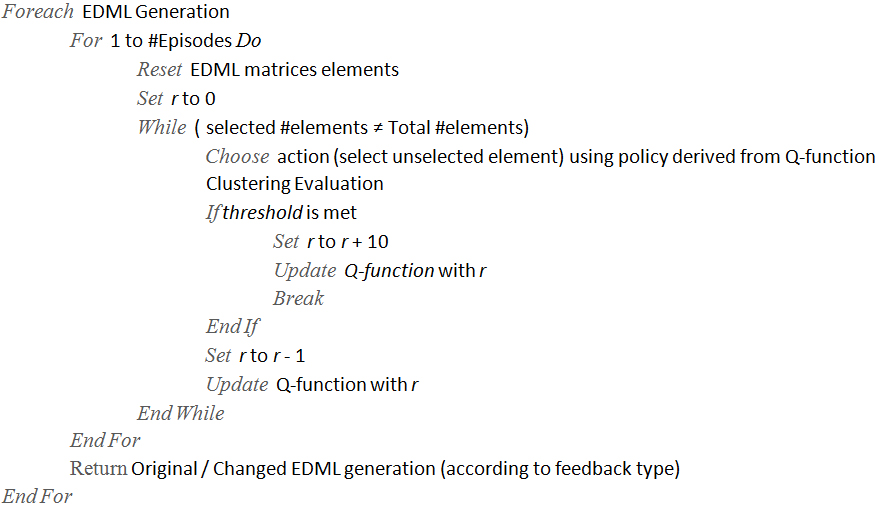

Figure 3.
R-EDML life cycle (diagonal R-EDML).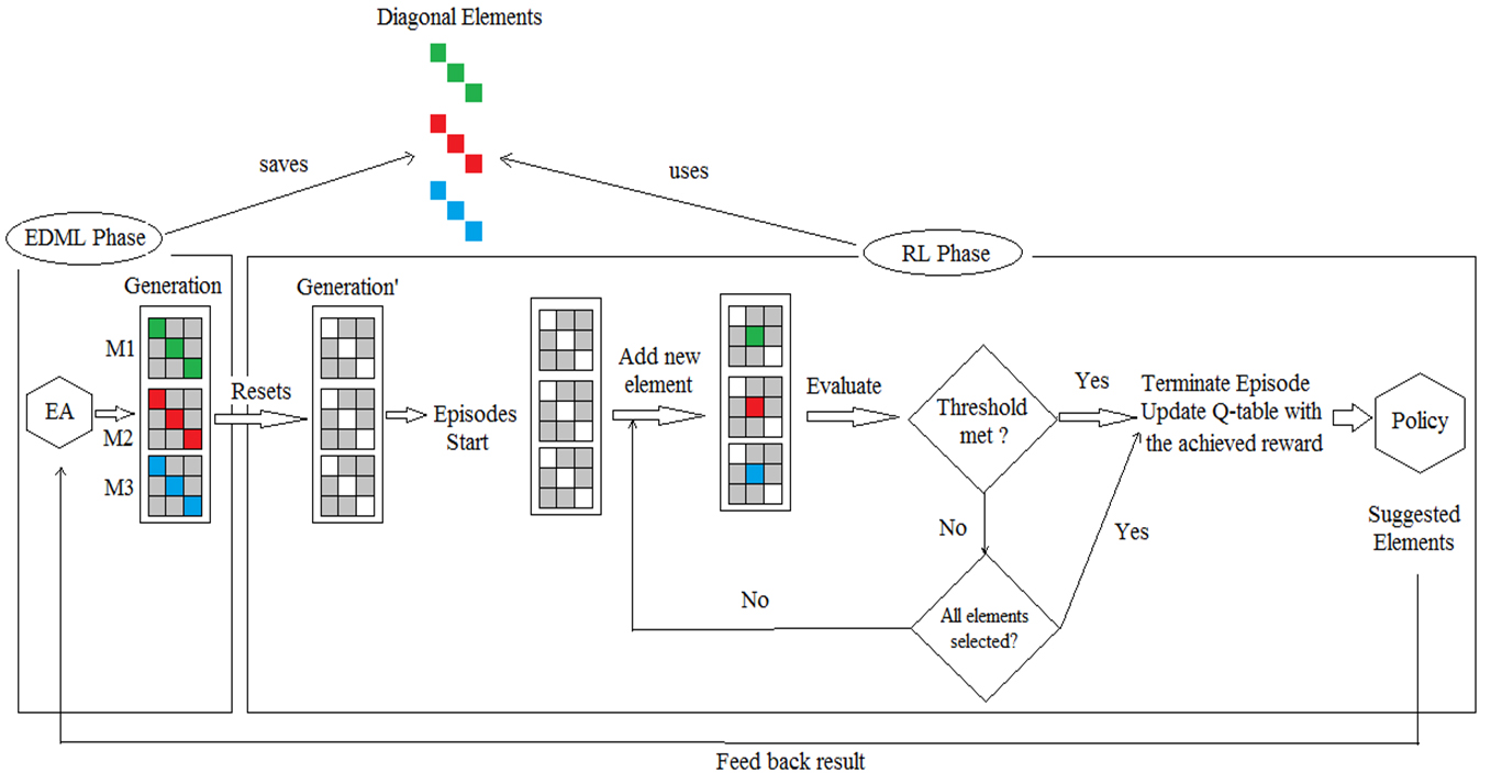

6. Experiments and results

	$T(\bm{x_{i}})=T(\bm{x_{j}})$	$T(\bm{x_{i}})\neq T(\bm{x_{j}})$
$C(\bm{x_{i}})=C(\bm{x_{j}})$	a	b
$C(\bm{x_{i}})\neq C(\bm{x_{j}})$	c	d

6.1 Overview

The goal of this section is to test the effect of the learned selection control strategy on the EDML transformation matrices. F-measure ( $F_{1}$ score) is used for clustering evaluation in the following experiments. To examine the different ways of combining EDML and RL in this hybrid system, a series of variations, scenarios, and experiments are tested on different real data sets. The results of R-EDML are compared with the embedded feature weighting conducted by EDML, which prioritizes the features, and also with the EDML accuracy [3] as well as conventional feature selection [4] to compare R-EDML with the original EDML as well as feature selection applied on EDML in terms of features number and accuracy. Since RL and EDML have a random factor in their processes, after the initial generation is created, it is saved to achieve a unified starting generation for all scenarios. Also, the average result for each test is taken. Moreover, policy separation is applied to all tests apart from the policy unification test, whereas Diagonal R-EDML is applied to all tests apart from the Full Matrix R-EDML test.

6.2 Tested scenarios

A multitude of approaches are tested and compared, the approaches are as follows: For each generation/N generations, Change/No Change EDML, Resettable/Appendable learning, learn from Policy (P)/Highest Accuracy (HA). The idea behind these scenarios is testing different ways of interaction between EDML and RL, some scenarios wait for EDML to converge first then change it or change EDML before it converges, others explore not changing EDML and run RL independently in parallel with it.

1.
For each generation/N generations: Since the RL phase runs on matrices, it is able to run any time independent from the EDML phase. Thus, we view the effect of how often the RL phase runs.

(a)
For each generation: Run RL for each EDML generation.
(b)
For every N generations: Run RL each time EDML finishes N generations.

2.
Change/No Change EDML: In this hybrid system, we test if the RL phase can offer better results by affecting the EDML phase or by running as an independent post process. It is believed in the early stages of EDML generations not to Change EDML as the generations are immature. The EDML should be changed after the generations are matured and are close to convergence.

(a)
Change EDML: After RL finishes with a generation, only the learned elements are passed on to the next generation and the rest is either set to zero (Change EDML 1) or reduced by a certain fixed ratio (0.2 $\times$ element value) (Change EDML 2).
(b)
No Change EDML: After RL finishes with a generation, all the elements pass on to the next generation. In that case, RL does not affect EDML; however, it acts as an observer that records the results and picks the best after learning.

3.
Resettable/Appendable learning: These scenarios test whether the next RL phase will perform better if affected by the previous RL phases. Resettable learning explores RL phases disconnected from one another, whereas Appendable learning connects RL phases.

(a)
Resettable learning: Before each RL episode starts, the generation matrices are reset from all the elements (Section 5.2, RL phase step b).
(b)
Appendable learning: Before each RL episode starts, the generation matrices are reset from all the elements except for the elements learned from the previous RL phases. After the current RL phase ends, the elements learned from the current RL phase are appended to the elements learned from the previous RL phases; and the next RL phase resets its elements except for these appended elements. This appending cycle will continue until the appended elements are equal to the total number of elements. In that case, the appended elements list will be emptied and the appending cycle starts again.

4.
Learn from Policy (P)/Highest Accuracy (HA): Two different RL phase outputs are explored; one uses the policy learned, and the second uses the highest result in the phase. The idea behind this is to check two types of feedback to EDML phase, one from the policy and the other from the episode with the best result.

(a)
Learn from Policy (P): For the current generation, after RL finishes its episodes, the learned elements are chosen by the RL policy described in Section 5.1.
(b)
Learn from Highest Accuracy (HA): For the current generation, after RL finishes its episodes, the learned elements are chosen from the HA episode in this phase.

5.
Frequent Items approach: This approach is tested to take advantage of elements frequently chosen in each RL phase. This feature is implemented to test whether better results will be achieved if these elements are fixed in the next phases. This feature is only implemented with Resettable option since the Appendable option forces the elements selected from the last RL phase to be added to the next RL phase. This approach works as follows: every element will have a frequency counter (initially 0). After every RL phase, if this element is selected as a learned element, its counter is incremented. Depending on a frequency threshold of 10, if an element’s counter reached this threshold, it will be added before each episode in the next RL phases.
6.
Merge technique approach: All the previous scenarios have been tested in different combinations but not all at the same time; this approach combines all of them. The idea is to examine the performance if EDML is unchanged by RL from the beginning and is allowed to mature and converge through the evolutionary process, and then RL is allowed to change it. This approach works as follows: given the total number of generations N, the RL phases acting on the first half of the generations will be No Change EDML with Resettable method, whereas the second half will be Change EDML with the Appendable method.

Figure 4 shows the process of No Change EDML, whereas Fig. 5 shows the process of both Change EDML and Change EDML 2. Moreover, Fig. 6 shows the Resettable learning approach, whereas Fig. 7 shows the Appendable learning approach. A multitude of combinations between the described scenarios in this section is tested. Figure 8 shows the Merge technique combinations, whereas Fig. 9 shows the normal (non Merge) scenarios combinations.

Figure 4.
Diagonal No Change EDML scenario: given a generation with 3 matrices (m1, m2, and m3), and each matrix has 5 diagonal elements, denoted by x. After the RL phase finishes, the generation is unchanged and is passed to the next EDML phase.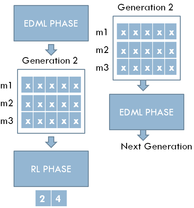

Figure 5.
Diagonal Change EDML scenarios: given a generation with 3 matrices (m1, m2, and m3), and each matrix has 5 diagonal elements, denoted by x. After the RL phase finishes and indices 2 and 4 are the elements learned. Before the EDML phase starts, the current generation matrices change where the learned elements keep their values, whereas the rest are either set to zero denoted by an empty cell (Change EDML 1) or reduced by a certain ratio denoted by a red x (Change EDML 2).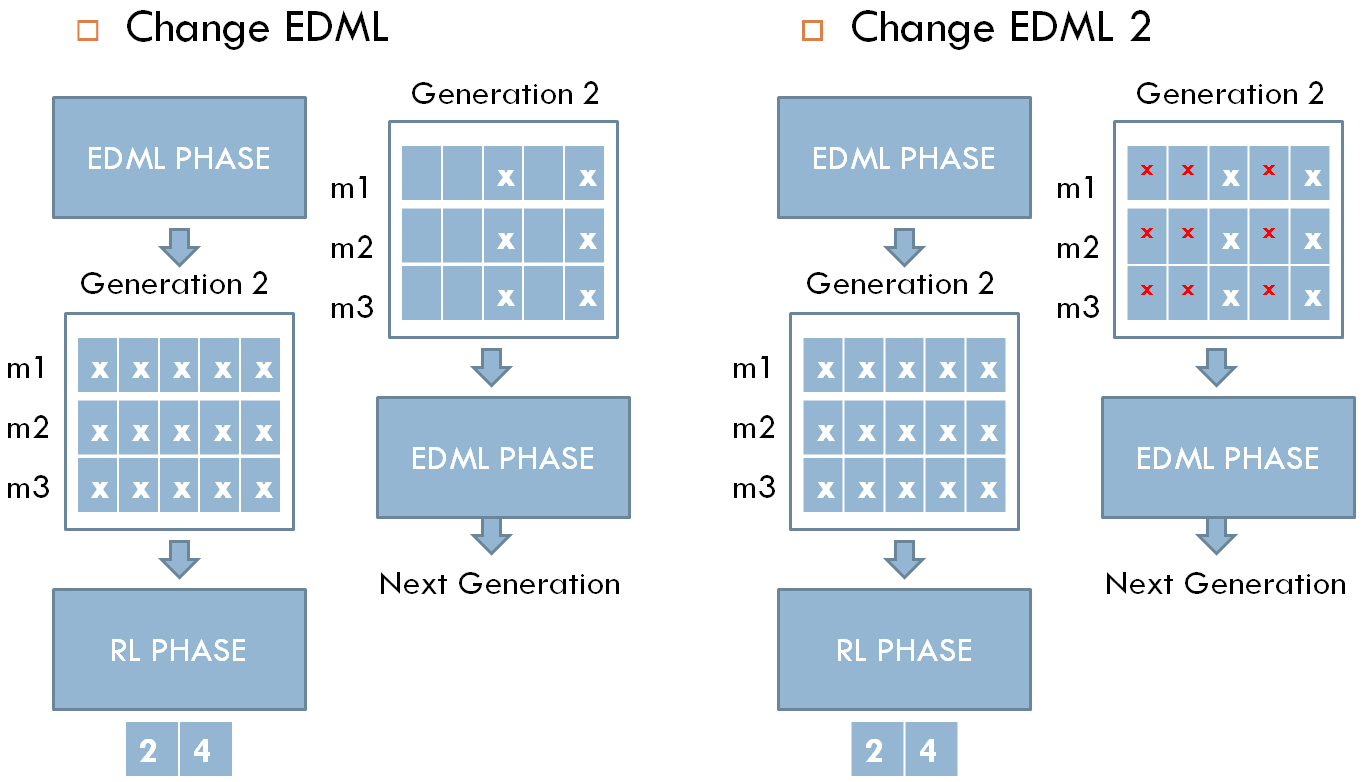

Figure 6.
Diagonal resettable learning scenario: in a generation with 3 matrices each (m1, m2, and m3), and each matrix has 5 diagonal elements. In the current RL phase and before every episode, the learned elements from the previous RL phase are not appended to the matrices.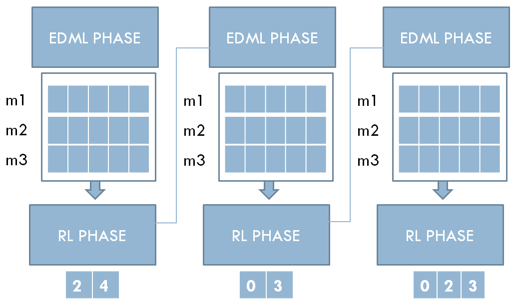

Figure 7.
Diagonal appendable learning scenario: in a generation with 3 matrices each (m1, m2, and m3), and each matrix has 5 diagonal elements. In the current RL phase and before every episode, the learned elements from the previous RL phase are appended to the matrices.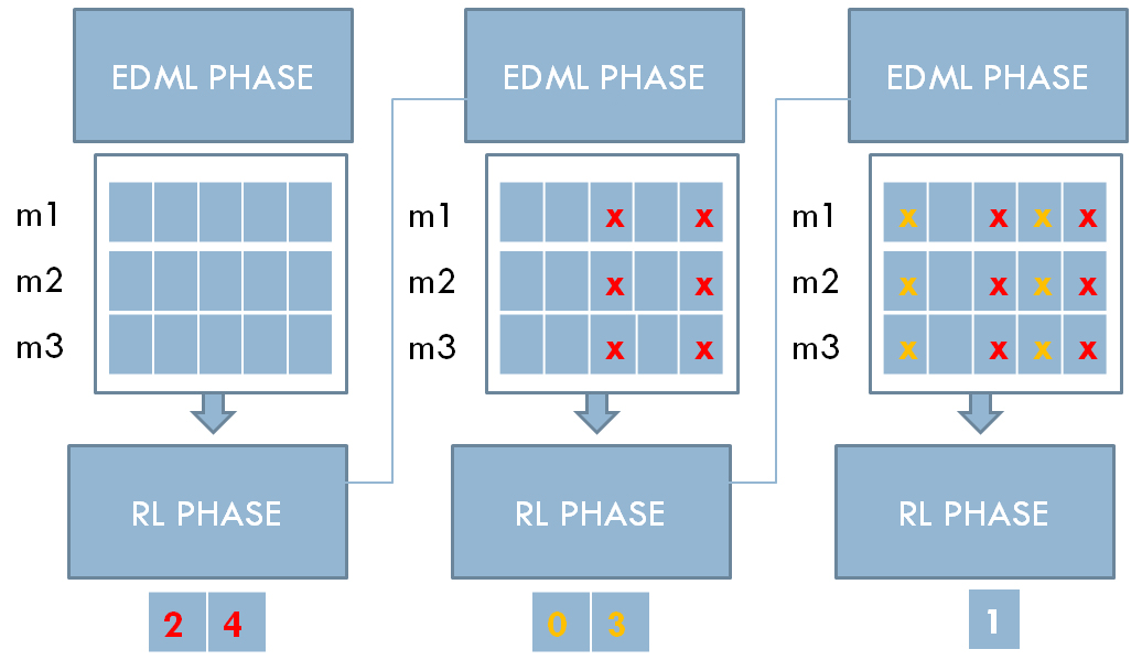

Figure 8.
Merge technique scenarios combinations.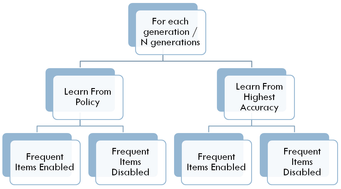

Figure 9.
Non Merge technique scenarios combinations.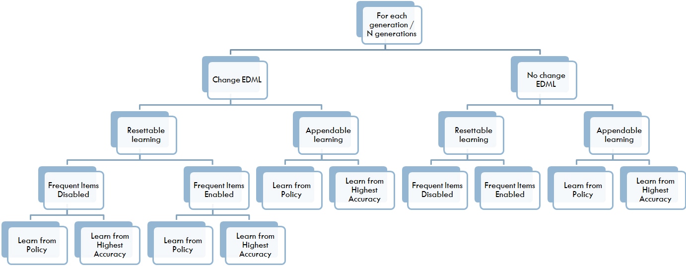

6.3 The employed database

The tests are carried out on the UCI machine learning database [5]. The data sets are Iris, Glass, Wine, Vehicle, and Segment; Iris data set contains 150 data points, 4 features, and 3 classes, Glass data set contains 214 data points, 9 features, and 6 classes, whereas Wine data set contains 178 data points, 13 features, and 3 classes. The Vehicle data set contains 846 data points, 18 features, and 4 classes. Finally, the Segment data set contains 2310 data points, 19 features, and 7 classes. The UCI data sets used in this research are used as is, i.e., we did not add any noise nor remove any values in the data sets. We choose those UCI data sets as they are reliable and they do not have missing values and are correctly labeled as well as containing little noise to consider in this research.

6.4 Experiment settings

Initial tests are carried out to filter out the best scenario combinations (described in Section 6.2) according to the best pair of accuracy and number of selected features. The tests are also conducted to choose the best margin $\phi$ in the RL threshold (described in Section 5.1). Tables 2–4 show the best 3 scenarios out of all the scenario combinations in Glass, Wine, and Vehicle data sets. The best-selected scenario to achieve the best pair of F-measure and number of features is the Merge technique with Change EDML 1 option, Frequency item enabled option, and For each 20 generations option [3]. In this study, multiple parameters are used owning to a hybrid system and combining multiple techniques like EDML and RL, each with their own set of hyperparameters as well as the parameters used for the scenarios. These parameters values are selected according to preliminary experiments and are divided as follows:

Table 2
Scenarios filtering in Glass data set

Scenario	F-measure	# Features
No Change EDML, Resettable [For each generation]	0.5344	3
Merge technique, Change EDML 1, Frequent Items [For each 20 generations]	0.5391	1
Change EDML 2, Resettable, Learn from Policy [For each 20 generations]	0.5324	1.9

Table 3

Scenarios filtering in Wine data set

Scenario	F-measure	# Features
No Change EDML, Resettable [For each generation]	0.879	4.2
Merge technique, Change EDML 1, Frequent Items [For each 20 generations]	0.955	3.3
Change EDML 2, Resettable, Learn from Policy [For each 20 generations]	0.9286	2.9

Table 4

Scenarios filtering in Vehicle data set

Scenario	F-measure	# Features
No Change EDML, Resettable [For each generation]	0.4453	2.2
Merge technique, Change EDML 1, Frequent Items [For each 20 generations]	0.4643	2.1
Change EDML 2, Resettable, Learn from Policy [For each 20 generations]	0.4538	1.6

EDML parameters: EDML parameters are used from previous papers [26, 27] which show after preliminary experiments that using these parameters will make EDML converge. Two thousand generations are created for each data set and each generation has a population of 20 matrices (Iris), 46 matrices (Glass and Wine), and 56 matrices (Vehicle and Segment). As for Full Matrix EDML, the population is 30 (Iris), 135 (Glass), 273 (Wine), and 513 (Vehicle and Segment). The number of clusters used in K-means is 20 (Iris, Glass, and Wine) or 50 (Vehicle and Segment).

RL parameters: Number of episodes per generation: 4 (in case of for each generation scenarios where N $=$ 1). The number of episodes per 20 generations: 40 (in case of for each N generations scenarios where N $=$ 20). Epsilon $=$ 0.1, AP (action punishment) $=$ $-$ 1, and TR (threshold reward) $=$ $+$ 10. The idea behind choosing these values is the following: The number of episodes is chosen according to preliminary experiments. As for the Epsilon value, it is set to 0.1 because the state-action space is not big to require a lot of exploration. For the rewards assignments, these values are selected after some preliminary experiments because it is believed that they are suitable for the range of features in the target data sets (4 to 19 features).

Scenarios parameters: Include the reduction fixed ratio of Change EDML 2 is set to 80% (described in Section 6.2) and the frequency threshold which is set to 10 with the idea that in case of for each generation, 100 RL phases will run and if an element is selected at least tenth of that number it will be considered frequent and important.

6.5 Experiments and tests

The following experiments use diagonal EDML, in which removing these elements is the same as removing features from the input space. The only exception is the Full Matrix R-EDML experiment that uses the entire EDML matrix. All experiments are performed 25 times and the average result is recorded for each data set.

6.5.1 R-EDML vs. EDML

The idea behind this experiment is to compare R-EDML to normal EDML to check if this hybrid system will improve EDML in terms of features and accuracy. EDML is used as a basis for comparison. Although EDML does not explicitly select features, it has its feature prioritizing process. We observed the EDML optimal matrices results and the ratios between all the elements’ weights and we picked a threshold of 0.05. The prioritizing method of EDML important features number is as follows: after all generations are created, the diagonal elements weights of the optimal matrix are analyzed. Weights that are less than the threshold (0.05) are immediately discarded, and the rest is filtered according to the following formula:

Given M* as the optimal EDML matrix with elements $m_{ii}^{*}$ , given $m_{\max}$ as the maximum value in M* and $m_{\min}$ as the minimum value in M* whose value is bigger than 0.1, $L^{*}$ is the list of prioritized important elements from M*. The following equation describes the EDML important feature prioritizing process:

$\displaystyle L^{*}=\{m_{ii}^{*}|m_{ii}^{*}\geqslant 0.05\text{ and }[(m_{\max% }-m_{ii}^{*})-(m_{\max}-m_{\min})]\leqslant 0.1\}$ (7)

6.5.2 R-EDML vs. conventional methods

Conventional feature selection is applied to EDML to test if it is superior to R-EDML in terms of feature reduction. Two types of feature selection are tested, both concentrate on different aspects of the features:

1.
Feature scoring: Gives score to each feature based on gain ratio [2] (Higher scores are better) and focuses on the quality of each feature.
2.
Feature subset selection: Uses greedy forward selection algorithm to select the best features and is based on Pearson’s correlation [12] that indicates the quality of the features, focusing on the relation between features instead of individual features.

6.5.3 Full Matrix R-EDML (non-diagonal)

Full Matrix R-EDML uses a combination of diagonal and non-diagonal elements. The purpose of this test is to take advantage of the Full Matrix capability in transforming the input space and see if the result can be improved while trying to use diagonal and non-diagonal elements. Full Matrix R-EDML is compared to another semi-supervised DML technique called Information-Theoretic Metric Learning (ITML) [15], which is the most famous DML method. A weight prioritizing process similar to that of EDML is carried out on ITML, later compared with R-EDML. A GitHub implementation1

¹
https://metric-learn.github.io/metric-learn/_modules/metric_learn/itml.html#ITML_Supervised.

is used for ITML.

6.5.4 R-EDML policy unification

In all the previous tests, in each R-EDML generation, a new policy tailored for the generation is learned because the assumption is that the R-EDML evolution algorithm changes and mutates the elements of each generation. In this experiment, the policy is unified across all generations to determine if a unified updated policy has potential validity.

6.6 Results and observations

Table 5 shows the feature weighting results of EDML and ITML, whereas Table 6 shows the comparison result between Full Matrix R-EDML and ITML. Tables 7–9 show the comparison between all the previous experiments among all data sets.

Table 5
Feature weighting results in EDML and ITML

Data set	# Feat.	EDML imp. feat.	ITML imp. feat.
Iris	4	2	2.1
Glass	9	3.3	3.7
Wine	13	6.3	6
Vehicle	18	3.6	7.4
Segment	19	4.8	6.8

Table 6

ITML comparison results

Data set	ITML (F-measure	# Feat.)	Matrix R-EDML (F-measure	# Feat.)
Iris	0.91	4	0.92	1.3
Glass	0.45	9	0.56	1.8
Wine	0.98	13	0.97	2.2
Vehicle	0.52	18	0.43	1.5
Segment	0.54	19	0.75	1

Table 7

F-measure comparison results

Data set	EDML	Feat. subset	Feat. scoring	R-EDML (policy sep)	R-EDML (policy uni)	Matrix R-EDML
Iris	0.92 $\pm$ 0.007	0.92 $\pm$ 0.006	0.91 $\pm$ 0.006	0.92 $\pm$ 0.004	0.92 $\pm$ 0.01	0.92 $\pm$ 0.003
Glass	0.54 $\pm$ 0.002	0.54 $\pm$ 0.001	0.53 $\pm$ 0.001	0.54 $\pm$ 0.002	0.54 $\pm$ 0.002	0.56 $\pm$ 0.003
Wine	0.95 $\pm$ 0.003	0.87 $\pm$ 0.007	0.93 $\pm$ 0.006	0.96 $\pm$ 0.009	0.93 $\pm$ 0.02	0.97 $\pm$ 0.007
Vehicle	0.43 $\pm$ 0.003	0.42 $\pm$ 0.002	0.44 $\pm$ 0.008	0.46 $\pm$ 0.01	0.46 $\pm$ 0.01	0.43 $\pm$ 0.003
Segment	0.72 $\pm$ 0.007	0.65 $\pm$ 0.01	0.73 $\pm$ 0.005	0.73 $\pm$ 0.009	0.73 $\pm$ 0.009	0.75 $\pm$ 0.008

Table 8

# Features comparison results

Data set	EDML	Feat. subset	Feat. scoring	R-EDML (policy sep)	R-EDML (policy uni)	Matrix R-EDML
Iris	4	2.5	2	1.4	1.4	1.3
Glass	9	4.5	3.5	1	1.2	1.8
Wine	13	5.5	7	3.3	1.4	2.2
Vehicle	18	3.5	6.5	2.1	1.6	1.5
Segment	19	4.5	12	1	1	1

Table 9

# Generations comparison results

Data set	EDML	Feat. subset	Feat. scoring	R-EDML (policy sep)	R-EDML (policy uni)	Matrix R-EDML
Iris	1244	786	956	778	486	870
Glass	1010	1146	989	726	482	786
Wine	1013	1174	1169	910	1098	948
Vehicle	473	101	322	464	390	98
Segment	441	267	354	376	359	392

In Table 9, # Generations refers to the number of generations needed to reach the best result (highest F-measure and lowest number of features), which is a measurement to verify the approach that converges faster.

In Table 8, # Features in Diagonal EDML refers to the number of the selected diagonal elements. In Full Matrix EDML, # Features refers to diagonal elements (whether these diagonal elements are explicitly selected by R-EDML or they are not explicitly selected but non-diagonal elements associated with these diagonal elements are selected; in this case, they are considered selected).

6.6.1 R-EDML vs EDML feature weighting

In Table 5, EDML EA important feature weighting has decreased the required features for every data set. Even though feature weighting is not a considered feature selection, EDML still uses all the features. Typically, R-EDML explicitly selected fewer features than EDML important features in Table 8.

6.6.2 Diagonal R-EDML vs Full Matrix R-EDML

Surprisingly, Full Matrix R-EDML selected fewer features than Diagonal R-EDML, even though the former used a Full Matrix instead of the diagonal one. In Table 8, Full Matrix R-EDML offered the best feature reduction in 3 out of 5 data sets as compared with the diagonal approach, where each policy method offered the least features in 2 out of 5 data sets. In Table 9, Full Matrix R-EDML converged faster in Vehicle data set, whereas in Iris, Glass, and Wine data sets Diagonal R-EDML converged faster. As for the F-measure, Table 7 shows that Full Matrix R-EDML offered better accuracy compared with Diagonal one, with higher accuracy in 3 out of 5 data sets.

6.6.3 Policy unification vs policy separation

In comparison to the policy separation approach, Table 8 shows that the unified policy selected fewer features in 2 out of 5 data sets, the same number of features in 2 out of 5 data sets and more features in only 1 data set. In terms of features, this shows better results. Regarding the F-measure, Table 7 shows that this approach offered the same accuracy in 4 out of 5 data sets. As for the number of generations to converge, Table 9 shows that the unified approach converged faster in 4 out of 5 data sets. This shows potential in the policy unification method.

6.6.4 R-EDML vs (EDML, feature subset and scoring)

R-EDML (Diagonal policy separation, Diagonal policy unification, and Full Matrix) showed better results in terms of F-measure, number of features, and convergence compared with conventional feature selection. In Table 7, R-EDML achieved better accuracy in all data sets. In Table 8, R-EDML selected fewer features in all data sets, and in Table 9, R-EDML needed a fewer number of generations to converge as it reached the best result in fewer generations in 4 out of 5 data sets. Thus, R-EDML feature selection strategy has led to a high average feature reduction % while keeping a high F-measure: 65% in Iris, 88% in Glass, 74% in Wine, 88% in Vehicle, and 94% in Segment. This shows that this method offers a great advantage.

6.6.5 Full Matrix R-EDML vs ITML

Since ITML uses a Full Matrix, only Full Matrix R-EDML is comparable to it. In Table 6, the comparative result is displayed for each data set showing the F-measure and the number of features. Even though ITML does not explicitly select features, but prioritize them instead, R-EDML selected fewer features than ITML. Since no advantage in F-measure between the two techniques is noted, we conclude that R-EDML is better than ITML.

6.7 Effect of the acceptance margin of F-measure

This section investigates the effect of the acceptance margin of F-measure ( $\phi$ in Section 5.1). We performed experiments on Wine and Glass data sets in the Diagonal R-EDML, while changing the control parameter. This parameter is the margin $\phi$ used in the threshold comparison to examine how the F-measure and the number of features change in the top three scenarios in Tables 2–4, i.e., No Change EDML, Merge, and Change EDML 2. Figure 10 shows the results of the two data sets using three different margins $\phi=$ 0.01, 0.04, and 0.08. Results show that as the value of the margin decreases, R-EDML gets an F-measure close to the best EDML accuracy. The results also show that as the F-measure increases, the number of features increases as well. When the value of the margin increases, R-EDML is not restricted with an accuracy close to the best accuracy; thus, the F-measure and the number of features decrease. Merge scenario showed better results compared with the other scenarios in both F-measure and number of features. Moreover, Merge scenario showed no increase in the number of features no matter how small the margin is in Glass data set, whereas in Wine data set, the number of features displayed a small increase when the margin is reduced compared with the other scenarios. This shows potential in RL in the EDML process (Merge) compared with running RL independently (No Change EDML).

Figure 10.

R-EDML margin evaluation graph.

7. Conclusion

In this paper, a hybrid system R-EDML is introduced that takes advantage of the sequential decision making in RL and the evolutionary process in EDML to produce an optimal distance metric with the same performance while extremely reducing the feature space. This approach reduces time complexity, saves future data collection time, and reduces the future cost of data collection since the unneeded features are costly or time-consuming. The experiments performed on UCI data sets show consistent superiority of R-EDML as they reduce the required features while maintaining or increasing the clustering performance when compared to the normal EDML and EDML with conventional feature selection. Full Matrix R-EDML is compared with ITML and produces good results. Similarly, R-EDML with policy unification is explored and achieves good results. These new changes in this hybrid system show promising potential and a chance for future improvements. For future work, it would be worth investigating the R-EDML performance on noisy data by adding synthetic noise to the UCI data as well as adding more performance measurements like Purity and Entropy.

Footnotes

Acknowledgments

This work was supported in part by the Network Joint Research Center for Materials and Devices.

References

A.Y.

, Feature selection, L1 vs. L2 regularization, and rotational invariance, in: Proc. The Twenty-first International Conference on Machine Learning (ICML), 2004.

Karegowda

A.G.

Manjunath

and Jayaram

, Comparative study of attribute selection using gain ratio and correlation based feature selection, International Journal of Information Technology and Knowledge Management 2(2) (2010), 271–277.

Ali

Fukui

Kalintha

Moriyama

and Numao

, Reinforcement learning based distance metric filtering approach in clustering, in: Proc. IEEE Symposium Series on Computational Intelligence (SSCI), 2017, pp. 1–8.

Ali

Kalintha

Moriyama

Numao

and Fukui

, Reinforcement learning for evolutionary distance metric learning systems improvement, in: Proc. the Genetic and Evolutionary Computation Conference Companion, 2018, pp. 155–156.

Blake

C.L.

and Merz

C.J.

, UCI Repository of machine learning databases, in: Department of Information and Computer Science, Vol. 55, 1998. http://www.ics.uci.edu/∼mlearn/MLRepository.html.

and Tian

, A comprehensive survey of clustering algorithms, in: Annals of Data Science, 2015, pp. 165–193.

Norouzi

Ahmadabadi

M.N.

and Araabi

B.N.

, Attention control with reinforcement learning for face recognition under partial occlusion, Machine Vision and Applications 22(2) (2011), 337–348.

Xing

E.P.

Jordan

M.I.

Russell

S.J.

and Ng

A.Y.

, Distance metric learning with application to clustering with side-information, in: Advances in Neural Information Processing Systems, 2003, pp. 521–528.

Rendon

Abundez

Arizmendi

and Quiroz

E.M.

, Internal versus external cluster validation indexes, in: International Journal of Computers and Communications, 2011, pp. 27–34.

10.

Wang

and Sun

, Survey on distance metric learning and dimensionality reduction in data mining, Data Mining and Knowledge Discovery 29(2) (2015), 534–564.

11.

Arnold

G.D.

Denoyer

Preux

and Gallinari

, Datum-wise classification: a sequential approach to sparsity, in: Proc. Joint European Conference on Machine Learning and Knowledge Discovery in Databases (EDML-PKDD), 2011, pp. 375–390.

12.

Chandrashekar

and Sahin

, A survey on feature selection methods, Computers & Electrical Engineering 40(1) (2014), 16–28.

13.

Hachiya

and Sugiyama

, Feature selection for reinforcement learning: Evaluating implicit state-reward dependency via conditional mutual information, in: Joint European Conference on Machine Learning and Knowledge Discovery in Databases, 2010, pp. 474–489.

14.

Brest

Greiner

Boskovic

Mernik

and Zumer

, Self-adapting control parameters in differential evolution: A comparative study on numerical benchmark problems, IEEE Transactions on Evolutionary Computation 10(6) (2006), 646–657.

15.

Davis

J.V.

Kulis

Jain

Sra

and Dhillon

I.S.

, Information-theoretic metric learning, in: Proceedings of the 24th International Conference on Machine Learning, ICML ’07, ACM, 2007, pp. 209–216.

16.

Janisch

Pevný

and Lisý

, Classification with costly features using deep reinforcement learning, in: Proc. the AAAI Conference on Artificial Intelligence, Vol. 33, 2019, pp. 3959–3966.

17.

Fukui

Ono

Megano

and Numao

, Evolutionary distance metric learning approach to semi-supervised clustering with neighbor relations, in: Proc. IEEE 25th International Conference on Tools with Artificial Intelligence (ICTAI), 2013, pp. 398–403.

18.

Fukui

and Numao

, Neighborhood-based smoothing of external cluster validity measures, in: Proc. Pacific-Asia Conference on Knowledge Discovery and Data Mining (PAKDD), 2012, pp. 354–365.

19.

Weinberger

K.Q.

and Saul

L.K.

, Distance metric learning for large margin nearest neighbor classification, Journal of Machine Learning Research 10(2) (2009), 207–244.

20.

Dash

and Liu

, Feature selection for classification, Intelligent Data Analysis 1(1–4) (1997), 131–156.

21.

Nezhad

M.Z.

Zhu

Yang

and Levy

, Safs: A deep feature selection approach for precision medicine, in: IEEE International Conference on Bioinformatics and Biomedicine (BIBM), 2016, pp. 501–506.

22.

Sutton

R.S.

and Barto

A.G.

, Reinforcement Learning: An introduction, in: MIT Press Cambridge, Vol. 1, 1998.

23.

Hertz

Bar-Hillel

and Weinshall

, Boosting margin based distance functions for clustering, in: Proc. The twenty-first International Conference on Machine Learning (ICML), 2004, p. 50.

24.

Nguyen

Silander

and Leong

T.Y.

, Online feature selection for model-based reinforcement learning, in: International Conference on Machine Learning, 2013, pp. 498–506.

25.

Rückstieß

, Reinforcement Learning in Supervised Problem Domains, PhD thesis, Universität München, 2016.

26.

Kalintha

Fukui

Ono

Megano

Moriyama

and Numao

, Semi-supervised Evolutionary Distance Metric Learning for Clustering, in: Proc. the 29th Annual Conference of The Japanese Society for Artificial Intelligence, 2015.

27.

Kalintha

Ono

Numao

and Fukui

, Kernelized evolutionary distance metric learning for semi-supervised clustering, in: Intelligent Data Analysis, Vol. 23, 2019, pp. 1271–1297.

Reinforcement learning based metric filtering for evolutionary distance metric learning

Abstract

Keywords

1. Introduction

2. Related work

2.1 Conventional feature selection

2.2 RL-based feature selection

3. EDML

4.1 RL overview

5.1 R-EDML model as an MDP

6.1 Overview

6.2 Tested scenarios

6.4 Experiment settings

Table 2 Scenarios filtering in Glass data set

6.5.1 R-EDML vs. EDML

1 https://metric-learn.github.io/metric-learn/_modules/metric_learn/itml.html#ITML_Supervised.

6.6 Results and observations

Table 5 Feature weighting results in EDML and ITML

6.6.2 Diagonal R-EDML vs Full Matrix R-EDML

6.6.3 Policy unification vs policy separation

6.6.4 R-EDML vs (EDML, feature subset and scoring)

6.6.5 Full Matrix R-EDML vs ITML

6.7 Effect of the acceptance margin of F-measure

Footnotes

Acknowledgments

References

Table 2
Scenarios filtering in Glass data set

¹
https://metric-learn.github.io/metric-learn/_modules/metric_learn/itml.html#ITML_Supervised.

Table 5
Feature weighting results in EDML and ITML