
Abstract
Bayesian network classifiers (BNCs) have proved their effectiveness and efficiency in the supervised learning framework. Numerous variations of conditional independence assumption have been proposed to address the issue of NP-hard structure learning of BNC. However, researchers focus on identifying conditional dependence rather than conditional independence, and information-theoretic criteria cannot identify the diversity in conditional (in)dependencies for different instances. In this paper, the maximum correlation criterion and minimum dependence criterion are introduced to sort attributes and identify conditional independencies, respectively. The heuristic search strategy is applied to find possible global solution for achieving the trade-off between significant dependency relationships and independence assumption. Our extensive experimental evaluation on widely used benchmark data sets reveals that the proposed algorithm achieves competitive classification performance compared to state-of-the-art single model learners (e.g., TAN, KDB, KNN and SVM) and ensemble learners (e.g., ATAN and AODE).
Keywords
Introduction
Machine learning, which has attracted widespread attention in recent years [1, 2, 3], is roughly divided into supervised learning and unsupervised learning. Nowadays, there are numerous supervised classifiers widely used in the real world [4, 5, 6, 7, 8, 9], among which Bayesian network classifiers (BNCs) is a popular approach due to their model interpretability and competitive classification performance [10, 11]. Formally, the topology of BNC learned from training data is a directed acyclic graph in which vertices correspond to the
Capital letters such as
For restricted BNC
Each factor in Eq. (1), i.e.,
In practice, most combinations of attribute values are either not represented in the training data or not present in sufficient numbers [17]. The network topology of BNC learned from labeled training data under the supervised learning framework may be unreliable and that may make it fail to generalize to fit unlabeled instances. To address this issue, researchers proposed to apply semi-supervised learning framework to use unlabeled testing instance in conjunction with labeled data for training. Existing semi-supervised approaches can be roughly grouped into four categories, including generative models [18], semi-supervised SVMs [19], graph-based semi-supervised methods [20, 21] and disagreement-based methods [22]. Some approaches, e.g., co-training and self-training, are universal and can work with any unspecified classifiers. Semi-supervised learning methods generally use unlabeled data to either modify or re-prioritize hypotheses obtained from labeled data alone. To achieve this goal, the unlabeled instance must be pre-assigned a class label first. Obviously, if the label is wrong, using such instance to re-train the classifiers learned from labeled training data will result in “noise propagation”, and the negative effect may lead to the biased decision boundaries. Moreover, the dependencies that exist in different instances may differ greatly. It is impossible for one single classifier to describe all “right” dependencies between attributes when they take specific values.
In this paper, we established the relationship between entropy function
This paper is organized as follows. In Section 2 we clarify the difference between NB and its variations in terms of log likelihood, and then review some state-of-the-art BNCs. In Section 3 we introduce the definitions of maximum correlation criterion and minimum dependence criterion, and then describe the basic idea of ensemble learning of two independent BNCs that respectively model training data and one single testing instance. In Section 4 we describe in detail the experimental setup and results of our proposed algorithm with other BNCs (including single model classifiers and ensemble classifiers). We conclude and outline future work in Section 5.
Given topology
Example of (a) full Bayesian network classifier, (b) Naive Bayes, (c) Tree augmented naive Bayes and (d) 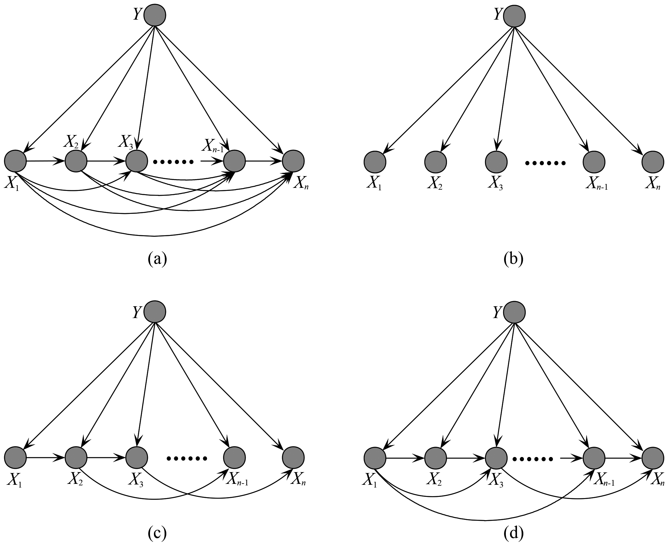
Because
As shown in Fig. 1a, suppose that the attribute order is
For NB, Eq. (3) turns to be
By comparing Eqs (3) with (5), the difference in amounts of bits between
NB has been demonstrated as a competitive alternative to other more complex classifiers especially when the data quantity is small. However, the independence assumption is often violated in practice, and as a result its probability estimates are often suboptimal. From Eq. (6), the strong conditional dependency relationship between any attribute
KDB (see Fig. 1d), which is proposed by Sahami [25], allows each attribute to be conditionally dependent on at most
Heuristic search strategy is commonly applied due to its efficiency in reducing the search space, but it may suffer from local optimal but global nonoptimal solutions. That is, the network topology learned from
Data sets
The value distributions of 
To represent such diversity, ensemble classifier seems to be a feasible solution. The difference among individual classifiers can adapt themselves to different instances, and most of the time lead the final ensemble classifier to perform as good as or better than the best individual classifier for a domain. ATAN [30] is proposed to improve the estimate of class probability in terms of conditional log likelihood. All attributes will be the root node in turn, resulting in a set of similar topologies with different directed arcs. WATAN [30] further improves ATAN by using the non-uniformly weighted average of the probability estimates, i.e., WATAN takes the mutual information between the root attribute and the class variable as the aggregation weight. To relax the independence assumption of NB while attaining the efficiency and efficacy of 1-dependence classifiers, AODE [31] utilizes a restricted class of one-dependence estimators (ODEs) and aggregates the predictions of these ODEs by using uniform rather than non-uniform weights. Further, subsumption resolution (SR) is proposed to optimize AODE by identifying pairs of attribute-values such that one is a generalization of the other and deletes the generalization [32].
Learn general BNC from training data
As shown in Fig. 1a, for full BNC there exists directed arc
After sorting attributes in descending order of
If
Thus when
We then sort the candidate parents of
SelectParents(
The KST
each
General BNC learned from training data makes unwarranted assumptions that, the relationship between
Ideally the learned BNC can take unlabeled instance
Then we need to learn a specific BNC, i.e., KST
Equation (13) implies that, to maximize the description of
For NB, Eq. (14) turns to be
By comparing Eqs (14) with (15), the difference in amounts of bits between
We can then learn the topology of KST
Similar to the learning procedure shown in Algorithm 2, to learn KST
Learning process of ensemble model.
As shown in Fig. 3, the pseudo training set is a complementary part of training set. Thus the probability distributions needed for computing
KST
From Eqs (8), (11) and (18), the estimate of the maximum correlation criterion and minimum dependence criterion is biased by the redundant attribute values or class labels that may not appear in
The experiments are conducted on 40 data sets from the UCI machine learning repository [33], and for these data sets it is supposed that there is no noisy data. As listed in Table 1, the size of data sets ranges from 57 instances of labor-negotiations to 164860 instances of localization, the number of class labels spans from 2 to 26, enabling us to evaluate classifiers on data sets with various sizes and wide range number of class labels. There exist missing values in 14 datasets. The Bayesian network classifiers for comparison study can deal with numeric attributes only, thus we discretize numeric attributes using Minimum Description Length (MDL) [34]. To incorporate the missing values into probability computation, we respectively use a distinct value to replace the missing values for qualitative attributes in all cases and the mean value to replace those missing ones for quantitative attributes. Consider the “noise” caused by the above data pre-processing steps, we hypothesize that there is sufficient data present for every possible combination of attribute values, and direct estimation of each relevant multi-variate probability will still be reliable for BNC learning.
Each algorithm is tested on each data set using 10 rounds of 10-fold cross validation. When two algorithms are compared, win/draw/loss (W/D/L) record is applied to compare the number of data sets on which one algorithm performs better/similarly/poorer than the other on a given measure. If the outcome of a one-tailed binomial sign test is less than 0.05, the difference is regarded as significant. The following algorithms are compared:
NB, standard naive Bayes. TAN, tree-augmented naive Bayes. KDB, ATAN, averaged tree-augmented naive Bayes. AODE, Averaged One-Dependence Estimators. KNN, SVM, Support Vector Machine with default parameters. KST,
These algorithms can be grouped into three types: single model BNCs (NB, TAN and KDB), ensemble BNCs (ATAN, AODE and KST) and non-BNC learners (KNN and SVM). For BNC learners, all the experiments use C
Zero-one loss is the most common loss function to evaluate the classification performance. Table A1 reports for each data set the average zero-one loss and Table 2 summarizes corresponding W/D/L records. Cell
W/D/L comparison results of 0–1 loss on all data sets
W/D/L comparison results of 0–1 loss on all data sets
The reasonableness of NB’s independence assumption is often questioned due to the non-negative characteristic of conditional mutual information. NB can only represent the direct dependence between any attribute
The Bias-variance decomposition provides valuable insights into the components of the error of learned classifiers [35]. Bias measures the deviation between the expected output of the learning algorithm and the real result, and describes the decision surfaces for a domain. Variance describes the component of error that stems from sampling, which reflects the sensitivity to variations in the training data.
Among single model BNCs, high-dependence BNCs enjoy significant advantage in representing conditional dependencies and correspond to more robust topologies. Due the ensemble learning strategy, ensemble BNC can represent more conditional dependencies than single model BNC of the same dependence degree. For example, TAN, KDB and AODE can respectively represent
W/D/L comparison results of bias on all data sets
W/D/L comparison results of bias on all data sets
W/D/L comparison results of variance on all data sets
Bias-variance trade-off is an important task in the field of statistics and machine learning, because it can make the model trained with limited training data better generalize to more data sets. Bias/variance estimation provides insights into how the learning algorithm will perform with varying amount of data. We expect low variance algorithms to have relatively low error for small data and low bias algorithms to have relatively low error for large data. The function, Goal Difference
where
W/D/L comparison results of RMSE on all data sets
The comparison results of GD in terms of (a) bias-variance and (b) 0–1 loss.
The Root-Mean-Square Error (RMSE) is a frequently used measure of the differences between values (sample or population values) predicted by a model or an estimator and the values observed. The RMSE represents the square root of the second sample moment of the differences between predicted values and observed values or the quadratic mean of these differences. The RMSE serves to aggregate the magnitudes of the errors in predictions for various times into a single measure of predictive power. RMSE is a measure of accuracy, to compare forecasting errors of different models for a particular data set and not between data sets, as it is scale-dependent.
The estimate of the conditional probability
Friedman test
The Friedman [37] and the Nemenyi [38] tests are effective for comparing multiple classifiers across multiple data sets. Classifier will be ranked by comparing their classification performance and the Friedman statistic is defined as follows:
where
Zero-one loss, RMSE, bias and variance comparison with the Nemenyi test on 40 data sets. CD 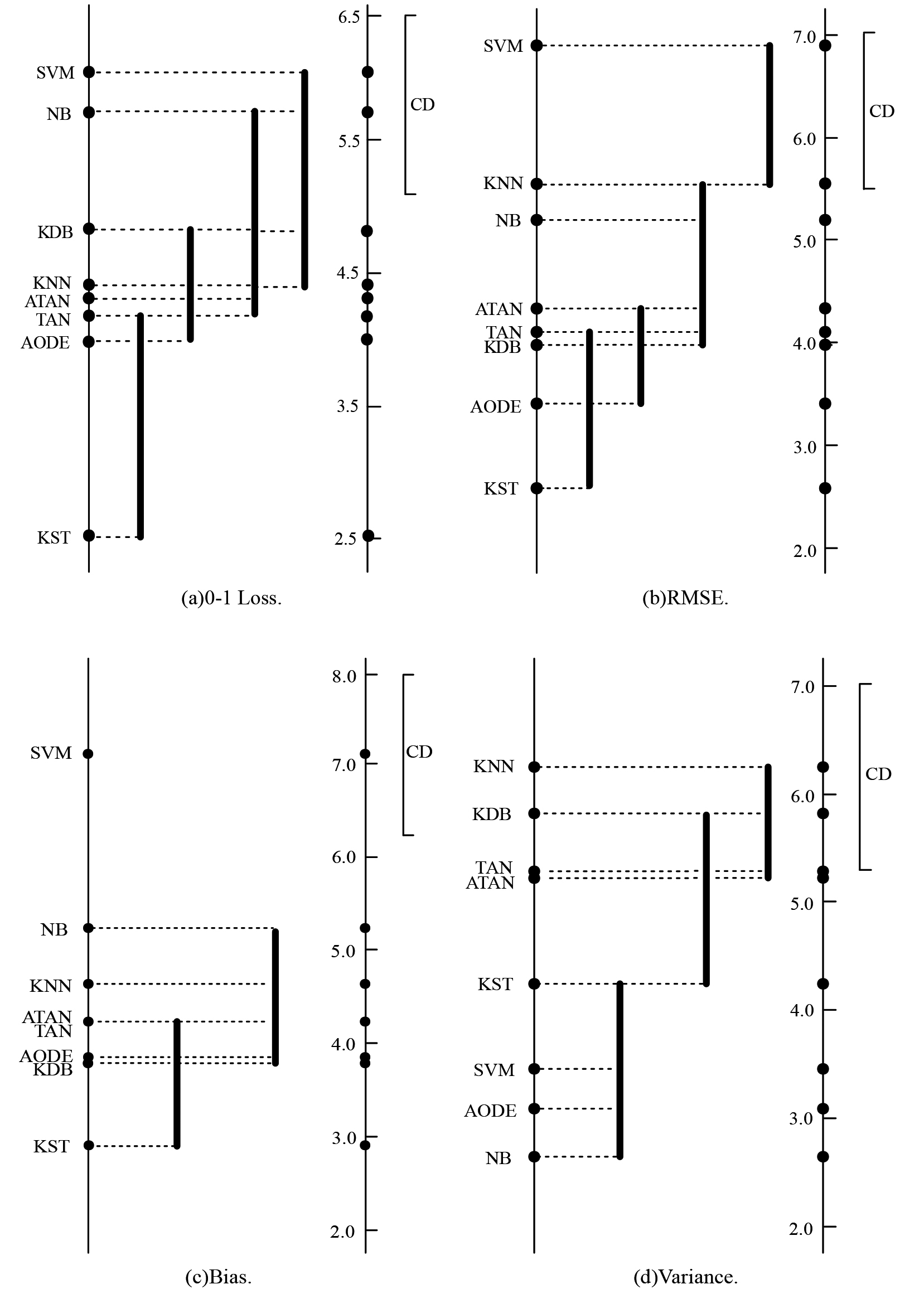
We can then use the Nemenyi test [38] to analyze if there exist significant difference between pairs of algorithms in terms of average ranks of the Friedman test. The critical difference (CD) is applied to evaluate the difference and is defined as follows:
where the critical value
As shown in Fig. 5a, KST achieves the lowest mean zero-one loss rank (2.5250) and the Nemenyi test differentiates KST from all the other algorithms. AODE, TAN, ATAN and KNN perform similarly, and they enjoy relatively significant zero-one loss advantage over KDB. NB and SVM obtain the highest rank among all the algorithms. In contrast, NB can only learns linear decision boundaries and underfitting make it fail to achieve the bias-variance trade off while dealing with large data sets. When RMSE is compared, from Fig. 5b KST and AODE achieve the lowest and second lowest mean RMSE ranks (2.5750 and 3.4000 respectively). KDB has lower rank than TAN, but the advantage is not significant. KNN and SVM obtain the highest variance rank among all the algorithms.
From Fig. 5c, KST obtains the lowest mean bias rank (2.9000), followed by KDB (3.8000) and AODE(3.8625). TAN, ATAN, KNN and NB come next (4.2250, 4.2250, 4.6250 and 5.2625 respectively). The bias disadvantages of SVM relative to other algorithms is clear. High-dependence relationships or ensemble learning has an obvious positive effect on reducing the bias of BNC. When variance is compared, from Fig. 5d NB has the lowest mean variance rank (2.6375). AODE and SVM have the second and the third lowest mean variance ranks (3.0875 and 3.4500 respectively). Although KST performs poorer than these three algorithms, it achieves significantly lower mean variance rank than TAN, ATAN, KNN and KDB.
Conditional mutual information
Footnotes
Appendix A
Experimental results of 0–1 loss
No.
Data set
NB
TAN
KDB
ATAN
AODE
KNN
SVM
KST
1
Contact-lenses
0.3750
0.3750
0.2500
0.4583
0.3750
0.2083
0.3750
0.3333
2
Zoo
0.0297
0.0099
0.0495
0.0198
0.0297
0.0396
0.0891
0.0297
3
Lymphography
0.1486
0.1757
0.2365
0.1757
0.1689
0.1892
0.1824
0.1757
4
Teaching-ae
0.4967
0.5497
0.5364
0.5497
0.4901
0.3377
0.5298
0.4570
5
Wine
0.0169
0.0337
0.0225
0.0337
0.0225
0.0506
0.5562
0.0225
6
Autos
0.3122
0.2146
0.2049
0.2195
0.2049
0.2390
0.6537
0.1902
7
Glass-id
0.2617
0.2196
0.2196
0.2150
0.2523
0.2103
0.2430
0.2196
8
Audio
0.2389
0.2920
0.3230
0.2965
0.2035
0.2301
0.5487
0.2257
9
Heart
0.1778
0.1926
0.2111
0.1926
0.1704
0.2444
0.4259
0.1815
10
Hungarian
0.1599
0.1701
0.1803
0.1701
0.1667
0.2313
0.3605
0.1565
11
Heart-disease-c
0.1815
0.2079
0.2244
0.2046
0.2013
0.2442
0.4323
0.1914
12
Primary-tumor
0.5457
0.5428
0.5723
0.5398
0.5752
0.6401
0.5605
0.5634
13
Ionosphere
0.1054
0.0684
0.0741
0.0684
0.0741
0.1368
0.0655
0.0684
14
Dermatology
0.0191
0.0328
0.0656
0.0328
0.0164
0.0546
0.1694
0.0273
15
Horse-colic
0.2174
0.2092
0.2446
0.2147
0.2011
0.2228
0.3370
0.1984
16
House-votes-84
0.0943
0.0552
0.0506
0.0529
0.0529
0.0759
0.0460
0.0506
17
Cylinder-bands
0.2148
0.2833
0.2259
0.2944
0.1889
0.2556
0.2333
0.1889
18
Balance-scale
0.2720
0.2736
0.2784
0.2752
0.2832
0.1344
0.1024
0.2624
19
Credit-a
0.1406
0.1507
0.1464
0.1522
0.1391
0.1884
0.4449
0.1420
20
Breast-cancer-w
0.0258
0.0415
0.0744
0.0443
0.0358
0.0443
0.0272
0.0415
21
Pima-ind-diabetes
0.2448
0.2383
0.2448
0.2383
0.2383
0.2982
0.3490
0.2396
22
Tic-tac-toe
0.3069
0.2286
0.2035
0.2276
0.2651
0.0125
0.1221
0.0710
23
Contraceptive-mc
0.5037
0.4888
0.5003
0.4888
0.4942
0.5567
0.4515
0.4915
24
Car
0.1400
0.0567
0.0382
0.0567
0.0816
0.0648
0.0810
0.0486
25
Mfeat-mor
0.3140
0.2970
0.3060
0.2990
0.3145
0.3450
0.6450
0.3050
26
Segment
0.0788
0.0390
0.0472
0.0403
0.0342
0.0286
0.3463
0.0368
27
Hypothyroid
0.0149
0.0104
0.0107
0.0104
0.0136
0.0291
0.0417
0.0111
28
Kr-vs-kp
0.1214
0.0776
0.0416
0.0776
0.0842
0.0372
0.0610
0.0635
29
Hypo
0.0138
0.0141
0.0114
0.0135
0.0095
0.0867
0.0740
0.0090
30
Sick
0.0308
0.0257
0.0223
0.0257
0.0273
0.0382
0.0610
0.0244
31
Phoneme
0.2615
0.2733
0.1984
0.2742
0.2392
0.2560
0.4071
0.2319
32
Wall-following
0.1054
0.0554
0.0401
0.0555
0.0370
0.1182
0.0971
0.0321
33
Page-blocks
0.0619
0.0415
0.0391
0.0422
0.0338
0.0398
0.0870
0.0327
34
Mushrooms
0.0196
0.0001
0.0000
0.0001
0.0001
0.0000
0.0020
0.0000
35
Sign
0.3586
0.2755
0.2539
0.2755
0.2821
0.1340
0.3273
0.2484
36
Nursery
0.0973
0.0654
0.0289
0.0654
0.0730
0.0162
0.0244
0.0481
37
Magic
0.2239
0.1675
0.1637
0.1674
0.1752
0.1906
0.3412
0.1568
38
Shuttle
0.0039
0.0015
0.0009
0.0015
0.0008
0.0007
0.0166
0.0009
39
Waveform
0.0220
0.0202
0.0256
0.0202
0.0180
0.0404
0.0271
0.0186
40
Localization
0.4955
0.3575
0.2964
0.3575
0.3596
0.2226
0.4209
0.2794
Experimental results of bias
No.
Data set
NB
TAN
KDB
ATAN
AODE
KNN
SVM
KST
1
Contact-lenses
0.2163
0.1825
0.3175
0.3137
0.2850
0.4352
0.4682
0.2838
2
Zoo
0.0318
0.0303
0.0403
0.0300
0.0273
0.0624
0.2022
0.0333
3
Lymphography
0.0902
0.1027
0.1041
0.0963
0.0933
0.1687
0.2802
0.1000
4
Teaching-ae
0.4836
0.4566
0.4606
0.4566
0.4370
0.3639
0.4843
0.4212
5
Wine
0.0331
0.0507
0.0520
0.0515
0.0346
0.0430
0.3955
0.0275
6
Autos
0.2181
0.2356
0.2253
0.2310
0.2165
0.2222
0.4871
0.2191
7
Glass-id
0.2901
0.2756
0.2713
0.2756
0.2785
0.1729
0.1810
0.2745
8
Audio
0.2733
0.3617
0.3493
0.3173
0.1753
0.2466
0.4860
0.2788
9
Heart
0.1368
0.1472
0.1697
0.1516
0.1403
0.1747
0.4826
0.1503
10
Hungarian
0.1646
0.1424
0.1480
0.1446
0.1582
0.1454
0.3878
0.1254
11
Heart-disease-c
0.1297
0.1263
0.1299
0.1267
0.1138
0.1360
0.3876
0.1106
12
Primary-tumor
0.4106
0.4249
0.4184
0.4244
0.4274
0.4307
0.5103
0.4226
13
Ionosphere
0.1220
0.0804
0.0855
0.0809
0.0744
0.1368
0.0973
0.0769
14
Dermatology
0.0079
0.0274
0.0489
0.0266
0.0055
0.0489
0.3482
0.0143
15
Horse-colic
0.1966
0.1848
0.1689
0.1963
0.1990
0.1717
0.3694
0.1898
16
House-votes-84
0.0899
0.0410
0.0258
0.0412
0.0430
0.0406
0.0331
0.0475
17
Cylinder-bands
0.2000
0.3117
0.1939
0.3217
0.1589
0.2012
0.3630
0.1548
18
Balance-scale
0.1840
0.1843
0.1902
0.1840
0.1905
0.1322
0.0971
0.1850
19
Credit-a
0.0912
0.1171
0.1137
0.1237
0.0921
0.1447
0.4637
0.0997
20
Breast-cancer-w
0.0187
0.0384
0.0449
0.0315
0.0338
0.0435
0.0257
0.0237
21
Pima-ind-diabetes
0.1957
0.1946
0.1944
0.1946
0.1937
0.1976
0.3359
0.1916
22
Tic-tac-toe
0.2614
0.1746
0.1367
0.1742
0.2005
0.0409
0.2041
0.0466
23
Contraceptive-mc
0.3928
0.3425
0.3702
0.3419
0.3816
0.3577
0.3568
0.3534
24
Car
0.0937
0.0478
0.0387
0.0478
0.0556
0.0799
0.1141
0.0451
25
Mfeat-mor
0.2624
0.2077
0.2142
0.2103
0.2477
0.2163
0.4895
0.2223
26
Segment
0.0785
0.0491
0.0453
0.0483
0.0367
0.0297
0.3957
0.0419
27
Hypothyroid
0.0116
0.0104
0.0096
0.0106
0.0094
0.0262
0.0449
0.0094
28
Kr-vs-kp
0.1107
0.0702
0.0417
0.0702
0.0747
0.0531
0.0812
0.0579
29
Hypo
0.0092
0.0124
0.0077
0.0120
0.0071
0.0619
0.0784
0.0087
30
Sick
0.0246
0.0207
0.0198
0.0208
0.0224
0.0354
0.0612
0.0220
31
Phoneme
0.2216
0.2394
0.1572
0.2360
0.2207
0.2088
0.7354
0.1854
32
Wall-following
0.0951
0.0491
0.0257
0.0490
0.0251
0.1105
0.1065
0.0232
33
Page-blocks
0.0451
0.0308
0.0280
0.0308
0.0251
0.0346
0.0894
0.0253
34
Mushrooms
0.0237
0.0001
0.0001
0.0001
0.0004
0.0000
0.0113
0.0002
35
Sign
0.3257
0.2420
0.2161
0.2417
0.2531
0.1140
0.3322
0.2129
36
Nursery
0.0928
0.0521
0.0281
0.0521
0.0651
0.0325
0.0535
0.0363
37
Magic
0.2111
0.1252
0.1241
0.1252
0.1600
0.1341
0.3404
0.1257
38
Shuttle
0.0040
0.0008
0.0007
0.0009
0.0006
0.0009
0.0371
0.0007
39
Waveform
0.0219
0.0152
0.0210
0.0152
0.0156
0.0245
0.0262
0.0152
40
Localization
0.4523
0.3106
0.2134
0.3105
0.3129
0.1671
0.4634
0.2084
Experimental results of variance
No.
Data set
NB
TAN
KDB
ATAN
AODE
KNN
SVM
KST
1
Contact-lenses
0.1712
0.1925
0.1700
0.1613
0.1275
0.1484
0.0540
0.1412
2
Zoo
0.0439
0.0606
0.0658
0.0548
0.0424
0.0745
0.1062
0.0485
3
Lymphography
0.0343
0.1116
0.1408
0.1118
0.0476
0.0815
0.0796
0.0755
4
Teaching-ae
0.1484
0.1914
0.1494
0.1914
0.1650
0.1932
0.1879
0.1848
5
Wine
0.0093
0.0493
0.0649
0.0502
0.0231
0.0299
0.2273
0.0319
6
Autos
0.1349
0.1747
0.1821
0.1704
0.1541
0.1988
0.2336
0.1706
7
Glass-id
0.0930
0.1075
0.1189
0.1075
0.1004
0.1182
0.1500
0.1170
8
Audio
0.1000
0.0983
0.1373
0.1613
0.1407
0.1295
0.2437
0.1439
9
Heart
0.0443
0.0739
0.0914
0.0751
0.0497
0.0813
0.0032
0.0663
10
Hungarian
0.0201
0.0596
0.0561
0.0585
0.0255
0.0863
0.0001
0.0470
11
Heart-disease-c
0.0248
0.0479
0.0582
0.0495
0.0357
0.0829
0.0908
0.0488
12
Primary-tumor
0.1752
0.2424
0.2391
0.2428
0.1814
0.2402
0.1596
0.2040
13
Ionosphere
0.0242
0.0401
0.0581
0.0422
0.0385
0.0361
0.0281
0.0325
14
Dermatology
0.0216
0.0513
0.0684
0.0496
0.0199
0.0546
0.1335
0.0389
15
Horse-colic
0.0353
0.1021
0.1384
0.1045
0.0452
0.0776
0.0019
0.0930
16
House-votes-84
0.0066
0.0170
0.0197
0.0167
0.0094
0.0218
0.0089
0.0152
17
Cylinder-bands
0.0656
0.0739
0.0750
0.0699
0.0961
0.1373
0.0511
0.1157
18
Balance-scale
0.0848
0.0941
0.0872
0.0938
0.0854
0.0831
0.0432
0.0852
19
Credit-a
0.0249
0.0555
0.0768
0.0589
0.0305
0.0663
0.0221
0.0464
20
Breast-cancer-w
0.0010
0.0337
0.0504
0.0372
0.0134
0.0169
0.0027
0.0273
21
Pima-ind-diabetes
0.0715
0.0663
0.0689
0.0663
0.0727
0.1134
0.0000
0.0677
22
Tic-tac-toe
0.0455
0.0824
0.1125
0.0823
0.0513
0.0591
0.0528
0.0606
23
Contraceptive-mc
0.0856
0.1646
0.1705
0.1644
0.1058
0.1947
0.1090
0.1565
24
Car
0.0520
0.0376
0.0434
0.0373
0.0438
0.0756
0.0370
0.0556
25
Mfeat-mor
0.0622
0.1020
0.1031
0.1015
0.0677
0.1031
0.2973
0.0924
26
Segment
0.0259
0.0294
0.0381
0.0285
0.0255
0.0259
0.2633
0.0265
27
Hypothyroid
0.0031
0.0034
0.0024
0.0031
0.0034
0.0109
0.0006
0.0024
28
Kr-vs-kp
0.0186
0.0152
0.0111
0.0152
0.0186
0.0559
0.0026
0.0176
29
Hypo
0.0051
0.0071
0.0069
0.0069
0.0049
0.0324
0.0003
0.0062
30
Sick
0.0047
0.0051
0.0043
0.0052
0.0042
0.0197
0.0008
0.0043
31
Phoneme
0.1215
0.1828
0.1064
0.1841
0.1343
0.1559
0.0295
0.1501
32
Wall-following
0.0211
0.0288
0.0294
0.0287
0.0242
0.0696
0.0390
0.0227
33
Page-blocks
0.0135
0.0143
0.0177
0.0144
0.0124
0.0194
0.0034
0.0132
34
Mushrooms
0.0043
0.0002
0.0002
0.0002
0.0001
0.0001
0.0010
0.0005
35
Sign
0.0313
0.0386
0.0596
0.0386
0.0378
0.0673
0.0210
0.0542
36
Nursery
0.0085
0.0168
0.0195
0.0167
0.0105
0.0582
0.0081
0.0177
37
Magic
0.0174
0.0490
0.0491
0.0490
0.0297
0.0707
0.0019
0.0427
38
Shuttle
0.0009
0.0004
0.0003
0.0004
0.0004
0.0006
0.0122
0.0003
39
Waveform
0.0009
0.0053
0.0037
0.0053
0.0025
0.0181
0.0026
0.0030
40
Localization
0.0460
0.0594
0.1099
0.0594
0.0580
0.0863
0.0192
0.1033
Experimental results of RMSE
No.
Data set
NB
TAN
KDB
ATAN
AODE
KNN
SVM
KST
1
Contact-lenses
0.3778
0.4496
0.3639
0.4101
0.4066
0.3165
0.5000
0.3904
2
Zoo
0.0802
0.0647
0.0859
0.0757
0.0677
0.0941
0.1596
0.0868
3
Lymphography
0.2446
0.2684
0.3031
0.2706
0.2478
0.2759
0.3020
0.2589
4
Teaching-ae
0.4789
0.4825
0.4804
0.4825
0.4670
0.4591
0.5943
0.4594
5
Wine
0.0926
0.1414
0.1211
0.1434
0.0976
0.1821
0.6089
0.1171
6
Autos
0.2714
0.2361
0.2323
0.2377
0.2324
0.2568
0.4322
0.2147
7
Glass-id
0.3540
0.3332
0.3395
0.3319
0.3439
0.3716
0.4025
0.3216
8
Audio
0.1254
0.1453
0.1528
0.1455
0.1194
0.1260
0.2138
0.1205
9
Heart
0.3651
0.3771
0.3949
0.3762
0.3569
0.4924
0.6526
0.3681
10
Hungarian
0.3667
0.3429
0.3552
0.3401
0.3476
0.4791
0.6005
0.3457
11
Heart-disease-c
0.3743
0.3775
0.3963
0.3767
0.3659
0.4924
0.6575
0.3590
12
Primary-tumor
0.1787
0.1814
0.1864
0.1815
0.1851
0.2243
0.2257
0.1799
13
Ionosphere
0.3157
0.2615
0.2714
0.2611
0.2506
0.3686
0.2560
0.2486
14
Dermatology
0.0631
0.0851
0.1206
0.0857
0.0692
0.1339
0.2376
0.0838
15
Horse-colic
0.4209
0.4205
0.4348
0.4217
0.4015
0.4706
0.5805
0.3899
16
House-votes-84
0.2997
0.2181
0.1969
0.2182
0.1994
0.2440
0.2144
0.2046
17
Cylinder-bands
0.4291
0.4358
0.4431
0.4469
0.4080
0.5045
0.4830
0.3786
18
Balance-scale
0.3260
0.3203
0.3177
0.3202
0.3199
0.2800
0.2613
0.3149
19
Credit-a
0.3350
0.3415
0.3480
0.3433
0.3271
0.4334
0.6670
0.3250
20
Breast-cancer-w
0.1570
0.1928
0.2497
0.1964
0.1848
0.1939
0.1649
0.1998
21
Pima-ind-diabetes
0.4147
0.4059
0.4074
0.4059
0.4078
0.5453
0.5907
0.4099
22
Tic-tac-toe
0.4309
0.4023
0.3772
0.4023
0.3995
0.2315
0.3495
0.2526
23
Contraceptive-mc
0.4506
0.4391
0.4485
0.4392
0.4398
0.5990
0.5486
0.4391
24
Car
0.2252
0.1617
0.1379
0.1616
0.2005
0.1953
0.2013
0.1541
25
Mfeat-mor
0.2086
0.1940
0.1974
0.1944
0.1985
0.2580
0.3592
0.1971
26
Segment
0.1398
0.0967
0.1034
0.0982
0.0879
0.0902
0.3146
0.0921
27
Hypothyroid
0.1138
0.0955
0.0937
0.0951
0.1036
0.1705
0.2043
0.0956
28
Kr-vs-kp
0.3022
0.2358
0.1869
0.2358
0.2638
0.1946
0.2470
0.2430
29
Hypo
0.0766
0.0738
0.0671
0.0734
0.0650
0.2081
0.1923
0.0627
30
Sick
0.1700
0.1434
0.1382
0.1434
0.1572
0.1953
0.2469
0.1425
31
Phoneme
0.0880
0.0902
0.0784
0.0902
0.0885
0.0915
0.1276
0.0846
32
Wall-following
0.2177
0.1586
0.1363
0.1588
0.1292
0.2430
0.2204
0.1192
33
Page-blocks
0.1450
0.1187
0.1128
0.1189
0.1021
0.1257
0.1865
0.1022
34
Mushrooms
0.1229
0.0083
0.0001
0.0082
0.0109
0.0000
0.0444
0.0195
35
Sign
0.3984
0.3505
0.3334
0.3504
0.3524
0.2892
0.4671
0.3363
36
Nursery
0.1766
0.1385
0.1121
0.1385
0.1571
0.1466
0.0988
0.1258
37
Magic
0.3974
0.3461
0.3470
0.3461
0.3541
0.4366
0.5841
0.3412
38
Shuttle
0.0298
0.0182
0.0146
0.0180
0.0126
0.0137
0.0689
0.0137
39
Waveform
0.1176
0.0951
0.1145
0.0951
0.0860
0.1641
0.1345
0.0894
40
Localization
0.2390
0.2095
0.1960
0.2095
0.2095
0.2012
0.2766
0.1881