Modeling data with observers

Abstract

Compact data models have become relevant due to the massive, ever-increasing generation of data. We propose Observers-based Data Modeling (ODM), a lightweight algorithm to extract low density data models (aka coresets) that are suitable for both static and stream data analysis. ODM coresets keep data internal structures while alleviating computational costs of machine learning during evaluation phases accounting for a O(n log n) worst-case complexity. We compare ODM with previous proposals in classification, clustering, and outlier detection. Results show the preponderance of ODM for obtaining the best trade-off in accuracy, versatility, and speed.

Keywords

Big data low density models coresets

1. Introduction

Data is a key resource for Artificial Intelligence (AI) applications since generalization and prediction require considerable volumes of information to build reliable Ground Truth (GT). In principle, and assuming a sufficient data quality, the more data available during Machine Learning (ML) training stages, the better the quality of the obtained models and classifications.

Managing, processing, and analyzing such ever-increasing volumes of data is a pressing challenge. Many algorithms either (1) cannot cope with massive raw data on-the-fly (freezing or collapsing) or (2) suffer from performance degradation due to noisy data, therefore requiring lightweight data summarization in between. For example, Zimek et al. show how sub-sampling in instance-based methods improves accuracy for outlier detection [46], introducing the counter-intuitive concept of “higher accuracy with less data”. Henceforth, data summaries become key middle boxes for future ML, either to understand data, avoid degradation, or to reduce computational costs. A way of summarizing data is by extracting a low density model from it, which is equivalent to what is commonly known as a coreset. A coreset is a subset $\mathcal{C}$ of data samples from an original set $\mathcal{X}$ that retains some characteristic properties for a given objective or fitting function $o(.)$ such that $o(\mathcal{C})\approx o(\mathcal{X})$ , as introduced by Agarwal et al. in [2].

To this end, we propose ODM, a lightweight algorithm for extracting low density data models that scales properly and helps to simplify and understand huge volumes of both static and stream data, creating optimized models for clustering, outlier analysis, and classification. ODM retrieves the idea of data observers presented in [43], which is a subset of data points used for approximating the original distribution, hence a coreset. Moreover, ODM admits some parameterization to adjust the granularity of the desired model and leverages the fact that observers do not necessarily have to be real data points.

The rest of this article is organized as follows. Section 2 explores similar methods and previous alternatives. Section 3 describes the ODM algorithm and presents its mathematical foundations. Experimental setups and datasets for the method evaluation are introduced in Section 4. Experimental results are shown and discussed in Section 5. Finally, the conclusions and a summary of the paper contributions are outlined in Section 6.

2. Related work

A way of understanding the processes that generate data is by finding simplified models that keep the underlying data structures with minimal amount of information. Regardless of the type of planned analysis, handling raw data is complex and time-demanding. Furthermore, because modern data is frequently noisy and unstable, data models are a suitable solution for eliminating unnecessary noise and retaining only the relevant structures, many times improving analysis performances [46]. Some research focuses on the task of extracting subsets from larger sets by using novel methods under a variety of objectives and constraints. Popular alternatives are listed below.

2.1 Statistics and error optimization

Among the most used, Bayesian coresets [28, 11, 12, 10] sample data with probabilistic models to create subsets that mimic the whole data in terms of approximating the posterior inference. The problem can be differently tackled with Gaussian Mixture Models [6, 36]; here the shape of the original data is reconstructed in a coreset by using a mixture of Gaussian functions whose parameters are adjusted accordingly. Feldman et al. [21] propose an alternative method that imposes constraints driven by Principal Component Analysis (PCA) and K-Means clustering. This method projects data into a low dimensional space, strategically selects some data points, and maps them back into the original space. The process ensures that both the whole dataset and the coreset yield similar principal components and centroids. Mirzasoleiman et al. [38] develop a technique for selecting a subset from a larger set with gradient-based learning algorithms. This method minimizes the error of an objective function in such a way that training with the entire dataset and the subset obtain the same error. Authors propose a greedy search algorithm to improve speed and avoid trying multiple combinations. The approaches introduced above build coresets very differently from each other, all of them also having a different theoretical basis from that used in ODM.

2.2 Distance-based methods

To generate coresets some methods combine smart data point sampling with measurements of point-to-point distances. For instance, Condensed Nearest Neighbor (CNN) [26, 4] was originally proposed as a solution for supervised training with a small number of representative samples. The algorithm is based on the 1-Nearest Neighbor label to retain only necessary samples and eliminate redundancy. The KMeans algorithm can also be used to find coresets [7] by extracting the shape of the input with a set of centroids that reflect major clusters in data. Finally, Iglesias et al. [43] mint the concept of “observers” to create a model of the data and use it later for detecting anomalies with the SDO (Sparse Data Observers) algorithm. Authors define observers as a set of sampled data points in which potential outliers have been removed according to a distance-based metric. These observers are later used as anchors to evaluate data points based on proximity calculations. ODM inherits the idea of “observers” from this work, but extends it by making them dynamically adaptable and controlling their generation and location. As a result, the set of observers in ODM is more density isotropic and homogeneous and less random.

2.3 Neural networks

Finally, techniques for extracting coresets with Neural Networks deserve a separate mention due to their peculiarities. Developed by Kohonen et al. [35], self-organizing maps (SOM) are strong alternatives for disclosing connections within multi-dimensional numerical data. They project complex input spaces into two-dimensional neural grids while trying to keep topological structures that are inherent to the original data. Based on SOM, Martinez et al. [37] propose Neural Gas and, later, Fritzke et al. present Growing Neural Gas [24]. These algorithms learn typologies by means of iterative fitting (or “growing”) processes. Intuitively, neurons behave like gas particles that extend and expand into the data, whose multidimensional shapes are seen as containers. This expansion of data points to occupy the entire space is analogous to the concept of low density models in ODM and play a similar role to the observers.

3. ODM

This section describes the ODM algorithm explicitly and with a few visual examples, shows its complexity and elaborates on its mathematical formulation. The algorithm framework is open-source and available in our git-hub repository.1

¹
github.com/CN-TU/pyodm.

Table 1 collects the notation and the algorithm parameters used throughout the paper.

Table 1

Notation

*	Symbol	**	Description
	$\mathcal{X}$	$-$	Dataset
	$\mathcal{C}$	$-$	Set of observers (coreset)
	$\mathcal{Y}$	$-$	Random subset of $\mathcal{X}$
	$\mathbf{x_{i}}$	$-$	Vector of the $i^{\text{th}}$ data point in $\mathcal{X}$
	$\mathbf{c_{j}}$	$-$	Vector of the $j^{\text{th}}$ observer in $\mathcal{C}$
	$\mathbf{y_{k}}$	$-$	Vector of the $k^{\text{th}}$ data point in $\mathcal{Y}$
	$n$	$\|\mathcal{X}\|$	Size of the data
✓	$m$	$-$	Size of the coreset
	$N$	$-$	Space dimensionality (number of features)
✓	$R_{o}$	$-$	Default radius of a new observer
	$R_{k}$	$-$	Radius of a $k^{\text{th}}$ observer
	$P_{j}$	$-$	Number of points assigned to the $j^{\text{th}}$ observer
✓	$f$	0.1	Expansion coefficient
✓	$\rho$	0.025	Sampling ratio for $R_{o}$ estimation
✓	$\beta$	1	Correction factor for $R_{o}$ estimation
✓	$\alpha$	1	Observer inertia coefficient
	$d(.)$	$-$	Distance metric
	$O(.)$	$-$	Time complexity
	$O_{m}$	$-$	Time complexity of ODM with m-Trees core
	$r$	$-$	Size ratio (%) between $\mathcal{C}$ and $\mathcal{X}$
	$\Delta u$	$-$	Displacement of an observer after an update

*: Algorithm parameter. **: Default value.

3.1 Observers

In [43], $\mathcal{C}$ (the observers set) is initially formed by randomly sub-sampling $\mathcal{X}$ . Authors define an observer as “a data object placed within the data mass and ideally equidistant to other observers within the same cluster”. Therefore, applied as models, observers are intended to evaluate data points from the input space that are located in their vicinity. We take this intuitive idea as a basis and modify concepts by giving observers some new properties. Here, observers are not required to be actual data points. Additionally, we assign to each observer $\mathbf{c_{j}}$ a maximum observation radius $R_{j}$ and a population $P_{j}$ , which accounts for the number of observed data points.

3.2 Algorithm

The goal of the ODM algorithm is to build a set of proper observers; aka an optimal coreset $\mathcal{C}$ that maximizes evaluation metrics compared to the original set and retains some characteristic properties for a given objective function $o(.)$ , as exposed in [2]. Therefore:

$\displaystyle o(\mathcal{C})\approx o(\mathcal{X})$ (1)

with $\mathcal{X}$ being the original set.

ODM starts taking a random data point as the first observer. Later, it processes the remaining data points sequentially as follows. Given a $i$ -data point ( $\mathbf{x_{i}}$ ),

•

if the distance to the closest observer ( $\mathbf{c_{j}}$ ) is below the radius of the observer ( $R_{j}$ ), $\mathbf{c_{j}}$ properties are modified to better fit the data (i.e., the radius $R_{j}$ is shrank and the location of $\mathbf{c_{j}}$ is slightly shifted toward $\mathbf{x_{i}}$ );

•

instead, if the distance is larger than the radius then $\mathbf{x_{i}}$ , it becomes a new observer.

Some parameters to comment on are:

•

$R_{o}$ (optional) is the default radius for any new observer. If not externally provided as a hyperparameter, $R_{o}$ is internally estimated (see 9). Large values of $R_{o}$ can cause superficial representations (very few observers), whereas very small values of $R_{o}$ reduce the compression rate and might result in more observers than necessary.

•

$f$ is an expansion factor that defines the growth rate of $R$ . Large values cause an unstable coreset construction in which observers jump over the space and do not converge properly, whereas low values give too much weight to observers, which barely update their locations and, therefore, more observers are required to cover all the data.

•

$\rho$ (required if $R_{o}$ is not given) is a sampling ratio used to estimate $R_{o}$ when this is not externally set. Higher values yield a better estimation but introduce a larger delay.

•

$m=|\mathcal{C}|$ (optional) is the number of observers (size of the coreset). If the size of the coreset is not externally imposed with this parameter, ODM internally optimizes it by itself.

•

$\alpha$ (optional) is a inertia coefficient that determines how observers update their locations. It enhances the configuration flexibility, but is a robust parameter set to 1 by default.

•

$\beta$ (optional) is a correction parameter for estimating $R_{o}$ . Also very robust, the default configuration gives optimal performances in most application cases.

(Required) $f$ , $R_{o}$ (Optional) $\rho$ , $m$ , $\alpha$ , $\beta$ $\mathcal{C}$ dataset $\mathcal{X}$

Shuffle $\mathcal{X}$ $R_{o}$ is not specified Estimate $\widehat{R_{o}}$ from $\mathcal{Y}$ , a fraction $\rho$ of $\mathcal{X}$ Set $R_{o}=\beta\widehat{R_{o}}$

Set a random sample $\mathbf{x_{r}}$ as $\mathbf{c_{0}}$ Set $P_{0}$ to $1$ Set $R_{0}$ to $R_{o}$ Append $\mathbf{c_{0}}$ to $\mathcal{C}$ $i$ in $|\mathcal{X}|-1$ Get $r$ the index of the nearest observer to $\mathbf{x_{i}}$ $d(\mathbf{c_{r}},\mathbf{x_{i}})\leqslant R_{n}$ Set $\Delta u$ to $\frac{\mathbf{x_{i}}-\mathbf{c_{r}}}{P_{r}+1}$ Shift $\mathbf{c_{r}}$ ’s coordinates by $\alpha\cdot\Delta u$ Increment $P_{r}$ by $1$ Subtract a fraction $f\cdot d(\mathbf{c_{r}},\mathbf{x_{i}})$ from $R_{r}$ Add a fraction $f\cdot d(\mathbf{c_{r}},\mathbf{x_{i}})$ to $R_{r}$ Create a new observer $\mathbf{c_{\text{new}}}=\mathbf{x_{i}}$ Set $P_{\textit{new}}$ to $1$ Set $R_{\textit{new}}$ to $R_{o}$ Append $\mathbf{c_{\text{new}}}$ to $\mathcal{C}$ $m$ is specified Sort $\mathcal{C}$ in descending order based on $P$ values first $m$ elements of $\mathcal{C}$ $\mathcal{C}$

ODM

Algorithm 3.2 shows the core routine of ODM, its mathematical formulation is discussed in Section 3.5. The process depicted in Algorithm 3.2, explained in a more intuitive way, goes though the following steps:

Shuffle the dataset (to avoid bias).

If $R_{o}$ is not adjusted as an external parameter, a random subset of the dataset ( $\mathcal{Y}$ ) is constructed with $|\mathcal{Y}|=\lceil n\rho\rceil$ elements. Then, $R_{o}$ is estimated as the average distance between all samples from $\mathcal{Y}$ and their corresponding centroid adjusted by a correction parameter $\beta$ .

The coreset is initialized with a first observer $\mathbf{c_{0}}$ , which is a randomly chosen data point from $\mathcal{X}$ . Hence, $R_{0}=R_{o}$ , and $P_{0}=1$ .

Later, the remaining data points are processed sequentially. For a given $\mathbf{x_{i}}$ , the algorithm calculates the distance between $\mathbf{x_{i}}$ and its closest observer $\mathbf{c_{j}}$ . If the distance is smaller than the observer radius $R_{j}$ , $\mathbf{c_{j}}$ is moved closer to $\mathbf{x_{i}}$ , its population $P_{j}$ increases by one and its radius $R_{j}$ is decreased by a fraction $f$ of the distance $d(\mathbf{c_{j}},\mathbf{x_{i}})$ . If, instead, the distance is larger, $\mathbf{x_{i}}$ becomes a new observer and $\mathbf{c_{j}}$ radius $R_{j}$ is increased by a fraction $f$ of the distance $d(\mathbf{c_{j}},\mathbf{x_{i}})$ .

The central loop of Algorithm 3.2 can be parallelized to enable faster extraction. Each data-batch is processed individually and the resulting subcoresets can be simply joined together afterwards. Moreover, the current implementation of ODM allows either omitting shuffling data points or picking them at random. Shuffling the data is useful when the arbitrary arrangement of data samples is to be ignored; otherwise, samples sorted by default might be prone to belong to the same cluster, and this could make observer radius to converge and shrink quickly, which ultimately creates more observers than needed. To avoid this, and to enable a better space reconstruction, data points should be picked at random. Finally, if the size of the coreset is externally fixed as a parameter ( $m$ ), the algorithm keeps only the $m$ -most populous observers for the final coreset.

Figure 1.

Two observers (in green) modeling a two-cluster dataset. Gradual observers locations are shown in blue.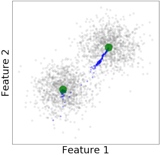

Figure 2.

Six observers (green) modeling a five-clusters dataset. Gradual observers locations are shown in blue.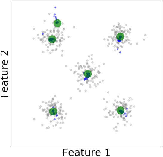

Figure 3.

Convergence path of an observer to the center of a sample cloud.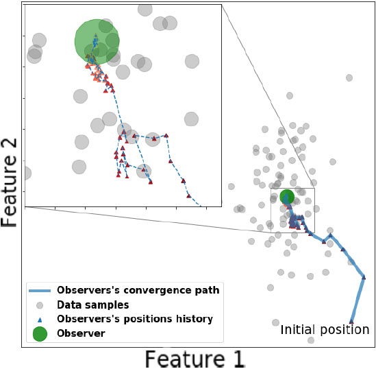

3.3 Examples

The operation of ODM can be better understood with a few simple examples. Figures 1 and 2 represent two datasets [22, 40] with two and five clusters. For these two cases ODM has been applied to obtain coresets with two and six points respectively. Data points are shown in gray-color, the final positions of observers in green, and the displacement of an observer is tracked with blue dots. We can see how observers end up in the respective clusters centers. If the number of observers is set to a higher number, the observers placement is expected to be distributed based on data density variations. We show a zoomed-in observer movement capture in Fig. 3 with a different dataset [23]. Here we can see that the observer placement converges and its displacement is progressively smaller.

The previous examples use very few observers in order to show the natural tendency of observers to be attracted by density centers. In practical modeling, higher granularity is commonly required, especially in cases with complex data structures. Figure 4 shows three datasets [32, 17, 42] for which ODM has been adjusted with low, medium, and high number of observers. As discussed above, denser coresets can be created by simply adjusting ODM parameters. Obviously, the size of a coreset cannot be larger than the size of the modeled dataset.

Figure 4.

ODM coresets extracted from three different datasets. Each column shows a parameterization with a different number of observers. Data points are shown in gray-color and observers in red.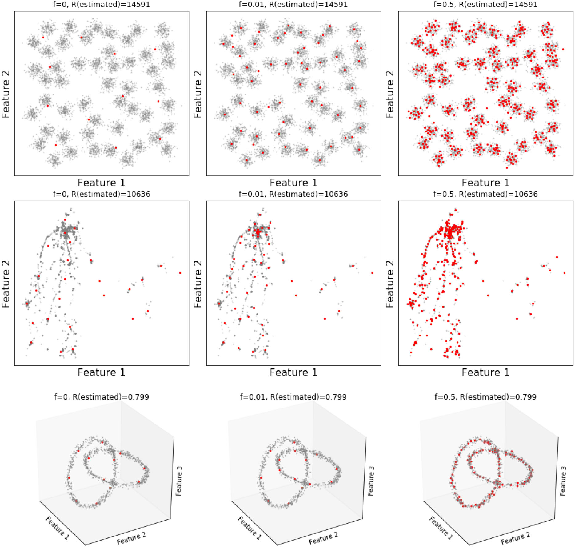

3.4 Complexity

The computational demand of ODM is mainly concentrated on the search of closest observers. Different algorithms can be used for this task; for instance kd-Trees [8] and m-Trees [15]. We opt for m-Trees in our implementation since they are robust, fast, and allow changes in the tree without need for reconstruction. The tree is built once at the beginning and keeps track of the observers. Based on Algorithm 3.2, each new data point involves: one k-nearest neighbor query, one insert (either a new observer or an updated one), and optionally one removal (remove an old observer if it has been updated and re-inserted). In the highly improbable average worst case scenario, which happens if the number of observers increases with each iteration and approaches the number of data points, the complexity $O_{m}$ with a m-Tree core can be estimated as follows: number of data points $\times$ (k-NN query $+$ removal $+$ insertion), which gives:

$\displaystyle O_{m}=O(n)\cdot[O(logn)+O(logn)+O(logn)]=\textbf{O(n log n)}$ (2)

$n$ being the number of processed data points (aka the cardinality of the dataset, $|\mathcal{X}|$ ).

3.5 Simplified mathematical formulation

In this section we address the mathematical formalism underlying ODM. ODM accepts different metrics for distance calculation (for instance, Aggrawal et al. [3] recommend using the Manhattan distances instead of Euclidean distances for high-dimensional spaces).

Initially, assuming that at least one observer exists in a coreset $\mathcal{C}$ , let $\mathbf{x_{i}}\in\mathbb{R}^{N}$ be the $i^{\text{th}}$ observation in an $N$ dimensional dataset $\mathcal{X}$ and let $\mathbf{c_{j}}\in\mathbb{R}^{N}$ be the closest observer to $\mathbf{x_{i}}$ :

$\displaystyle\mathbf{x_{i}}=\left[\begin{array}[]{c}x_{i,0}\\ x_{i,1}\\ \vdots\\ x_{i,N}\\ \end{array}\right]\quad\mathbf{c_{j}}=\left[\begin{array}[]{c}c_{j,0}\\ c_{j,1}\\ \vdots\\ c_{j,N}\\ \end{array}\right]$ (3)

If the distance between $\mathbf{c_{j}}$ and $\mathbf{x_{i}}$ is smaller than $R_{j}$ :

$\displaystyle d(\mathbf{c_{j}},\mathbf{x_{i}})\leqslant R_{j}$ (4)

The coordinates of $\mathbf{c_{j}}$ are updated such:

$\displaystyle\mathbf{c_{j}}\leftarrow\mathbf{c_{j}}+\alpha\Delta\mathbf{u}$ (5)

Where $\alpha$ is the observer’s inertia coefficient that controls the displacement (set to 1 by default) and $\Delta\mathbf{u}$ is the displacement defined as:

$\displaystyle\Delta\mathbf{u}=\frac{\mathbf{x_{i}}-\mathbf{c_{j}}}{P_{j}+1}$ (6)

$P_{j}$ is the number of data points associated to the observer $\mathbf{c_{j}}$ (i.e., observations/population) and $\mathbf{x_{i}}-\mathbf{c_{j}}$ is a distance vector. An observer $\mathbf{c_{a}}$ with high population is called lazy observer since the displacement when observing a new data point tends to vanish, i.e.,:

$\displaystyle\lim_{P_{a}\to\infty}\Delta\mathbf{u}=\lim_{P_{a}\to\infty}\frac{% \mathbf{x}-\mathbf{c_{a}}}{P_{a}+1}=\mathbf{0}$ (7)

Equation (7) shows that after many iterations, more observers become lazy and their location tends to be bounded in a smaller region in the output space. Moreover, Eq. (7) always holds since the distance vector $\mathbf{x}-\mathbf{c_{a}}$ cannot be arbitrarily large (in comparison to $P_{a}+1$ ) nor exceeds the radius of the observer (Eq. (4)). The additional $+1$ in the denominator is utilized to make sure that an observer with population $P=1$ is moved half the distance to the data sample observed.

The radius of the closest observer is at the same time updated regardless of the distance check performed in Eq. (4):

$\displaystyle R_{j}\leftarrow\max\Big{(}R_{j}\pm f\times d(\mathbf{c_{j}},% \mathbf{x_{i}}),0\ \Big{)}$ (8)

Depending on the distance check, the radius $R_{j}$ of an observer $\mathbf{c_{j}}$ is increased or decreased by a fraction $f$ of the distance between the current sample ( $\mathbf{x_{i}}$ ) and the closest observer ( $\mathbf{c_{j}}$ ) itself. Conversely the $max(.,0)$ operator ensures that the radius is always positive.

Figure 5.

By applying Eq. (9), the initial radius 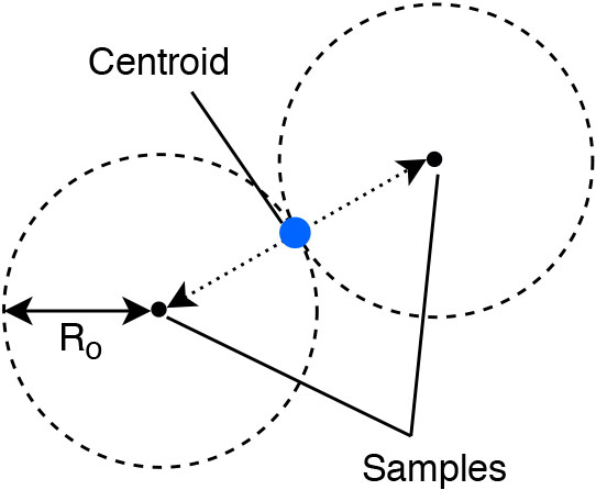$R_{o}$ is estimated to be the radius of circles centered at each sample and optionally corrected using $\beta$ ( $=1$ in this case).

If not specified as an external parameter, the initial radius of new observers is estimated as follows:

$\displaystyle R_{o}=\beta\left(\frac{1}{|\mathcal{Y}|}\sum_{j}^{|\mathcal{Y}|}% d(\mathbf{y_{j}},\bar{\mathbf{y}})\right)$ (9)

Whereby $|\mathcal{Y}|=\lceil n\rho\rceil$ . Equation (9) computes the average distance to the centroid of samples in a set $\mathcal{Y}$ sampled from $\mathcal{X}$ . $\beta$ is a tunable correction parameter (set to 1 by default). Figure 5 shows how $R_{o}$ is estimated in the case of a two-points subset.

4. Experiments

In this section we describe experiments conducted to evaluate ODM. They are tasks related to anomaly detection, clustering, and supervised classification. In the experiments, ODM is compared with alternative coreset extraction algorithms (described in Section 2), namely:

•
Baseline. No coreset, the whole dataset is used instead.
•
RS. A coreset obtained by uniform Random Samping.
•
SDO. Sparse Data Observers [43].
•
KMC. k-Means Coreset [7].
•
BGM. Bayesian Gaussian Mixture [36].
•
GNG. Growing Neural Gas [24].
•
CNN. Condensed Nearest Neighbours [26, 4] (only for supervised classification).

4.1 Datasets

For the experiments we used public datasets that are commonly applied for algorithm testing in the literature. A prerequisite when selecting datasets was that they should contain a considerable number of samples in order to make the application of coresets meaningful. The datasets used are:

•
MDCG-datasets. Fifteen datasets created with MDCGen [29], a tool for the highly-customized generation of multi-dimensional, multi-cluster datasets for algorithm testing. Parameters were selected to obtain scenarios with different number of dimensions, clusters, sample sizes, cluster overlap, and noise.
•
OTDT-datasets. A set of six popular datasets for outlier detection collected from the literature [25, 1, 9, 20, 34, 45]. They are imbalanced datasets with two possible classes: normal and anomalies (or inliers and outliers). The positive class corresponds to anomalies, which account for less than 10% of the total dataset size.
•
MCC-datasets. A set of five modern and balanced classification dataset with binary and multi-class targets (up to 10 classes) are used for the classification task [18, 31, 33, 14, 16].
•
Toy-datasets. Some real and synthetic datasets (up to 3 dimensions) selected from the literature to illustrate characteristics of the algorithm under study [32, 17, 42, 22, 40, 23].

Table 2 shows characteristics (max and min values) of each family of datasets. The noise level is calculated as the percentage of outliers. Whenever a dataset showed missing values, the corresponding vector was removed from the analysis. “na” stands for cases in which the GT was not given by dataset publishers, therefore such values depend on the algorithm used for analyzing the dataset.

Table 2
Datasets characteristics

Datasets Samples Dimensions Clusters/classes Ouliers Noise (%) Missing values

MDCG 1050–5250 2–20 2–20 50–300 1.96–9.09 None

OTDT 214–286048 3–27 2 9–3511 0.03–7.41 Dropped

MCC 4839–20867 5–11 2–11 na na Dropped

Toy 158–13467 2–3 1–51 na na None

4.2 Anomaly detection

Datasets	Samples	Dimensions	Clusters/classes	Ouliers	Noise (%)	Missing values
MDCG	1050–5250	2–20	2–20	50–300	1.96–9.09	None
OTDT	214–286048	3–27	2	9–3511	0.03–7.41	Dropped
MCC	4839–20867	5–11	2–11	na	na	Dropped
Toy	158–13467	2–3	1–51	na	na	None

Figure 6.

Scheme of the anomaly detection experiments.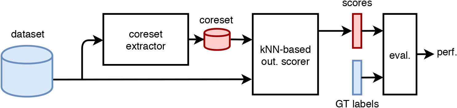

Coresets can help anomaly detection to alleviate the computational cost of instance-based methods and avoid degradation [46]. The traditional way of measuring outlierness is by considering the whole dataset (or all previous data points) when evaluating each single data point. Instead, with coresets each single data point is contrasted only with the coreset to decide if it is considered as anomaly, therefore considerably reducing the computational burden. The experiment methodology is shown in Fig. 6, its elements are described as follows:

•

Datasets. We used OTDT-datasets (Section 4.1).

•

Coreset extractors. Competitor algorithms were tuned to create coresets with different $r$ values (0.5%, 1%, 5% and 10%), where $r$ is the size of the coreset relative to the dataset size, i.e.,

$\displaystyle r=\frac{|C|}{|\mathcal{X}|}\cdot 100=\frac{m}{n}\cdot 100$ (10)

Since anomaly detection is unsupervised learning, additional parameters of each algorithm are tuned with the default values suggested in the respective references.

•

Outlierness scorer. We use the kNN-based outlier detection algorithm proposed by Ramaswamy et al. [39] to obtain outlierness scores. The number of neighbors is set to five ( $k=5$ ).

•

Evaluator. We evaluate performance by computing the P@n, average precision, ROC-AUC and MaxF1 scores using the GT labels as suggested by [13]. We show adjusted metrics to allow fair comparisons regardless of the number of outliers. We additionally measure coreset extraction and k-NN-based outlierness scoring (empirical) average runtimes.

The setup shown in Fig. 6 covers 144 experimental runs (6 algorithms $\times$ 6 datasets $\times$ 4 $r$ values) in addition to the baseline variant. Experiments results are summarized in Table 3 and discussed in Section 5.1.

4.3 Clustering

Figure 7.

Scheme of the clustering experiments.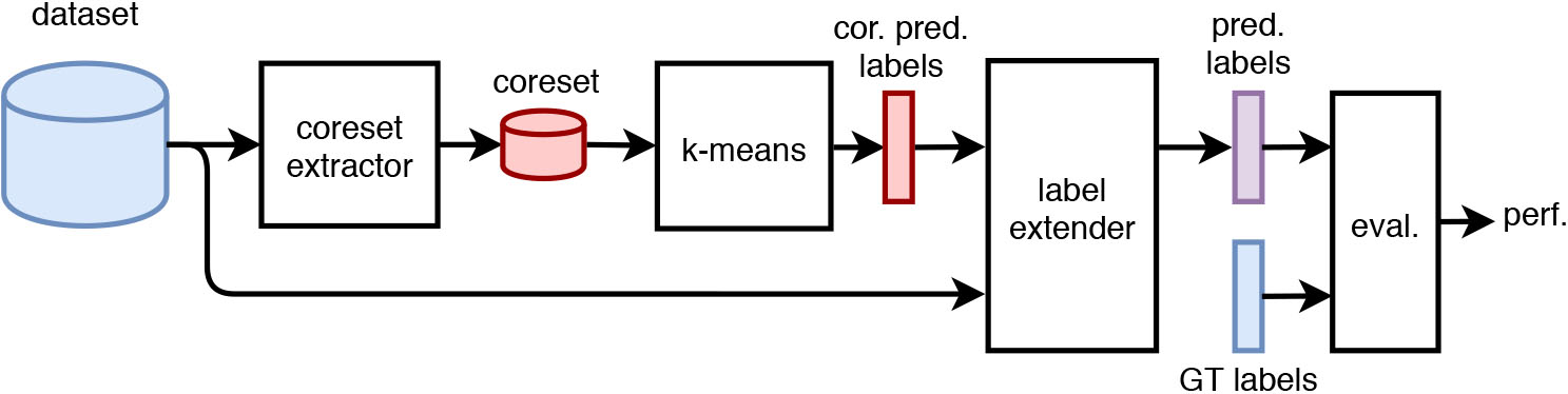

Similarly to the anomaly detection case, in order to reduce memory and time requirements, label assignment in clustering can be performed by clustering a coreset and extending labels to the whole dataset based on proximity calculations. We reproduced this scheme in our experiments and used k-means as core algorithm. The methodology is shown in Fig. 7. Elements are:

•

Datasets. We used MDCG-datasets (Section 4.1).

•

Coreset extractors. Competitor algorithms were tuned with different $r$ values (0.5%, 1%, 5% and 10%). Again, additional algorithm parameters were tuned based on the default values suggested in source references

•

k-means. Clustering is undertaken by the k-means++ algorithm [5]. The initial number of cluster $k$ is assumed as a known value prior to the analysis.

•

Label extender. This block calculates coreset cluster centers (centroids) and assigns final labels to the whole dataset by extending the label of the closest center (1-NN distance metric).

•

Evaluator. We evaluate performances with the external validity rand index [27] between predicted labels and GT labels and the internal validity silhouette score [41]. We additionally measure coreset extraction, k-means and label extender (empirical) average runtimes.

The setup shown in Fig. 7 covers 360 experimental runs (6 algorithms $\times$ 15 datasets $\times$ 4 $r$ value) in addition to the baseline variant. Experiments results are summarized in Table 4 and discussed in Section 5.2.

4.4 Supervised classification

Figure 8.

Scheme of the supervised classification experiments.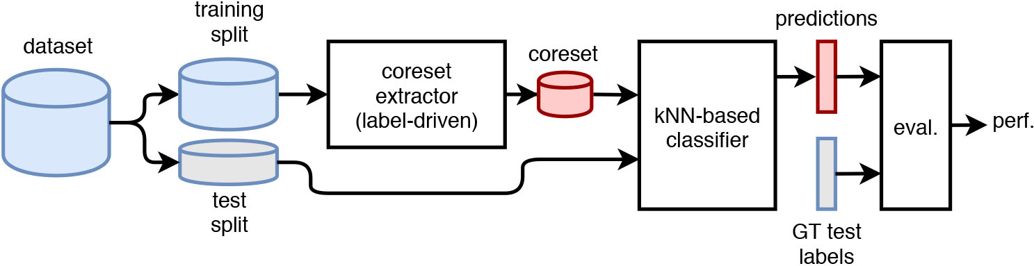

Coresets can also be used in supervised classification for data reduction, therefore suppressing noise, favoring generalization, and reducing training and/or evaluation complexity. Here coresets are intended to retain the essential set of training points for the subsequent classification. Note that such data reduction is strongly recommended for instance-based (aka lazy) learners that deal with large datasets, in which the coreset would work as a model and make it closer to eager learning options. This approach would be consistent with the sampling recommendations given by Zimek et al. in [46] for the anomaly detection case. In our experiments we reproduce the setup with the following blocks (Fig. 8):

•

Datasets. We used MCC-datasets (Section 4.1). We divided each dataset in training (70%) and test (30%) splits with stratified sampling. Datasets show different categories, therefore this becoming a multiclass classification experiment.

•

Coreset extractors. Competitor algorithms were tuned again with different $r$ values (0.5%, 1%, 5% and 10%). “label-driven” means that training data was divided into subsets based on GT labels and coresets were consequently extracted from each subset and later joined. This setup was used for all algorithms, except for CNN, which is already designed to properly deal with multiclass data. Also, vanilla CNN cannot be adjusted to create coresets with specific number of datapoints; therefore, random sampling was applied as a last step to equalize CNN with other algorithms and allow fair comparisons.

Other algorithm parameters were adjusted by using Evolutionary search on training data.

•

k-NN based classifier. We use a vanilla kNN-classifier to predict labels. The number of neighbors is set to five ( $k=5$ ).

•

Evaluator. We provide accuracy as well as micro and macro precision and recall metrics. We additionally measure coreset extraction and k-NN-based classification (empirical) average runtimes.

The setup shown in Fig. 8 covers 140 experimental runs (7 algorithms $\times$ 5 datasets $\times$ 4 $r$ values) in addition to the baseline variant. Experiments results are summarized in Table 5 and discussed in Section 5.3.

5. Results and discussion

In this section, we show and discuss results obtained from the experimental evaluation.

5.1 Anomaly detection

Results in Table 3 support the claims in [46] and show that, as a general rule, sub-sampling data improves the accuracy of outlier detection algorithms, since the baseline approach (i.e., using the whole dataset) performs worse than experiments that use coresets regardless of the used technique and the considered metric. Beyond that, all studied algorithms seem to obtain representative coresets for the analysis, KMC, SDO, and ODM slightly standing out over the rest.

Table 3
Performance of detecting anomalies

Algorithm	r	MaxF1	Adj-MaxF1	P@tn	Adj-P@tn	AP	Adj-AP	ROC-AUC	Ext. Time (s)		k-NN Time (s)
Baseline	0%	0.32 $\pm$ 0.08	0.29 $\pm$ 0.10	0.14 $\pm$ 0.12	0.11 $\pm$ 0.10	0.19 $\pm$ 0.16	0.16 $\pm$ 0.15	0.83 $\pm$ 0.09	–		5.47 $\pm$ 5.44
ODM	0.5%	0.45 $\pm$ 0.23	0.42 $\pm$ 0.24	0.23 $\pm$ 0.25	0.21 $\pm$ 0.25	0.26 $\pm$ 0.25	0.23 $\pm$ 0.24	0.86 $\pm$ 0.12	2.26	$\pm$ 2.32	2.64 $\pm$ 2.77
RS		0.38 $\pm$ 0.17	0.35 $\pm$ 0.19	0.17 $\pm$ 0.16	0.14 $\pm$ 0.15	0.22 $\pm$ 0.19	0.19 $\pm$ 0.18	0.81 $\pm$ 0.12	0.00	$\pm$ 0.00	2.77 $\pm$ 2.98
SDO		0.43 $\pm$ 0.23	0.40 $\pm$ 0.24	0.23 $\pm$ 0.26	0.20 $\pm$ 0.26	0.27 $\pm$ 0.26	0.24 $\pm$ 0.26	0.85 $\pm$ 0.12	0.24	$\pm$ 0.32	2.64 $\pm$ 2.78
KMC		0.44 $\pm$ 0.21	0.41 $\pm$ 0.22	0.25 $\pm$ 0.27	0.22 $\pm$ 0.26	0.27 $\pm$ 0.27	0.25 $\pm$ 0.26	0.83 $\pm$ 0.12	23.27	$\pm$ 30.69	2.70 $\pm$ 2.81
WGM		0.38 $\pm$ 0.24	0.35 $\pm$ 0.25	0.23 $\pm$ 0.29	0.20 $\pm$ 0.29	0.25 $\pm$ 0.27	0.23 $\pm$ 0.27	0.78 $\pm$ 0.13	228.49	$\pm$ 331.62	2.67 $\pm$ 2.79
GNG		0.40 $\pm$ 0.19	0.37 $\pm$ 0.19	0.23 $\pm$ 0.25	0.20 $\pm$ 0.24	0.25 $\pm$ 0.24	0.22 $\pm$ 0.23	0.83 $\pm$ 0.12	433.36	$\pm$ 589.89	2.82 $\pm$ 2.89
ODM	1%	0.41 $\pm$ 0.17	0.38 $\pm$ 0.18	0.20 $\pm$ 0.19	0.17 $\pm$ 0.18	0.24 $\pm$ 0.21	0.22 $\pm$ 0.20	0.84 $\pm$ 0.10	2.43	$\pm$ 2.44	2.77 $\pm$ 2.86
RS		0.38 $\pm$ 0.17	0.35 $\pm$ 0.18	0.17 $\pm$ 0.14	0.14 $\pm$ 0.13	0.22 $\pm$ 0.18	0.19 $\pm$ 0.17	0.82 $\pm$ 0.11	0.00	$\pm$ 0.00	2.73 $\pm$ 2.81
SDO		0.41 $\pm$ 0.18	0.38 $\pm$ 0.19	0.19 $\pm$ 0.18	0.16 $\pm$ 0.17	0.22 $\pm$ 0.19	0.19 $\pm$ 0.18	0.84 $\pm$ 0.11	0.43	$\pm$ 0.56	2.70 $\pm$ 2.82
KMC		0.40 $\pm$ 0.18	0.37 $\pm$ 0.19	0.18 $\pm$ 0.16	0.15 $\pm$ 0.15	0.22 $\pm$ 0.19	0.19 $\pm$ 0.18	0.83 $\pm$ 0.10	47.00	$\pm$ 59.96	2.82 $\pm$ 2.95
WGM		0.38 $\pm$ 0.23	0.35 $\pm$ 0.24	0.22 $\pm$ 0.27	0.19 $\pm$ 0.27	0.23 $\pm$ 0.27	0.21 $\pm$ 0.27	0.79 $\pm$ 0.12	414.47	$\pm$ 637.57	2.75 $\pm$ 2.89
GNG		0.41 $\pm$ 0.18	0.38 $\pm$ 0.19	0.21 $\pm$ 0.20	0.18 $\pm$ 0.20	0.23 $\pm$ 0.21	0.21 $\pm$ 0.20	0.83 $\pm$ 0.11	796.74	$\pm$ 1109.50	2.71 $\pm$ 2.82
ODM	5%	0.40 $\pm$ 0.16	0.37 $\pm$ 0.18	0.17 $\pm$ 0.14	0.14 $\pm$ 0.13	0.22 $\pm$ 0.18	0.19 $\pm$ 0.17	0.84 $\pm$ 0.10	2.41	$\pm$ 2.45	3.26 $\pm$ 3.29
RS		0.39 $\pm$ 0.16	0.36 $\pm$ 0.18	0.18 $\pm$ 0.14	0.14 $\pm$ 0.13	0.23 $\pm$ 0.19	0.20 $\pm$ 0.18	0.83 $\pm$ 0.10	0.00	$\pm$ 0.00	3.05 $\pm$ 3.09
SDO		0.38 $\pm$ 0.15	0.35 $\pm$ 0.17	0.17 $\pm$ 0.14	0.14 $\pm$ 0.12	0.22 $\pm$ 0.18	0.19 $\pm$ 0.17	0.83 $\pm$ 0.10	1.82	$\pm$ 2.34	3.32 $\pm$ 3.35
KMC		0.41 $\pm$ 0.20	0.38 $\pm$ 0.21	0.16 $\pm$ 0.13	0.13 $\pm$ 0.12	0.21 $\pm$ 0.17	0.18 $\pm$ 0.16	0.81 $\pm$ 0.11	241.52	$\pm$ 325.97	3.49 $\pm$ 3.45
WGM		0.26 $\pm$ 0.14	0.23 $\pm$ 0.16	0.08 $\pm$ 0.07	0.04 $\pm$ 0.05	0.13 $\pm$ 0.12	0.10 $\pm$ 0.10	0.72 $\pm$ 0.12	2134.30	$\pm$ 3212.13	3.01 $\pm$ 3.25
GNG		0.28 $\pm$ 0.07	0.25 $\pm$ 0.07	0.16 $\pm$ 0.14	0.13 $\pm$ 0.12	0.22 $\pm$ 0.18	0.19 $\pm$ 0.17	0.81 $\pm$ 0.10	3344.25	$\pm$ 4983.34	2.87 $\pm$ 2.93
ODM	10%	0.39 $\pm$ 0.16	0.36 $\pm$ 0.18	0.16 $\pm$ 0.13	0.13 $\pm$ 0.12	0.22 $\pm$ 0.18	0.19 $\pm$ 0.17	0.84 $\pm$ 0.10	2.27	$\pm$ 2.34	3.07 $\pm$ 3.09
RS		0.39 $\pm$ 0.16	0.36 $\pm$ 0.18	0.16 $\pm$ 0.13	0.13 $\pm$ 0.12	0.21 $\pm$ 0.18	0.19 $\pm$ 0.16	0.84 $\pm$ 0.10	0.00	$\pm$ 0.00	3.02 $\pm$ 3.04
SDO		0.39 $\pm$ 0.16	0.36 $\pm$ 0.18	0.16 $\pm$ 0.13	0.13 $\pm$ 0.12	0.22 $\pm$ 0.19	0.20 $\pm$ 0.17	0.83 $\pm$ 0.10	2.56	$\pm$ 3.33	2.88 $\pm$ 2.94
KMC		0.38 $\pm$ 0.18	0.35 $\pm$ 0.19	0.16 $\pm$ 0.13	0.12 $\pm$ 0.11	0.21 $\pm$ 0.17	0.18 $\pm$ 0.16	0.81 $\pm$ 0.11	359.22	$\pm$ 497.37	3.15 $\pm$ 3.13
WGM		0.27 $\pm$ 0.14	0.24 $\pm$ 0.16	0.11 $\pm$ 0.09	0.07 $\pm$ 0.09	0.16 $\pm$ 0.13	0.12 $\pm$ 0.12	0.72 $\pm$ 0.12	3884.61	$\pm$ 6105.35	3.36 $\pm$ 3.86
GNG		0.27 $\pm$ 0.10	0.24 $\pm$ 0.09	0.16 $\pm$ 0.13	0.12 $\pm$ 0.11	0.19 $\pm$ 0.17	0.17 $\pm$ 0.15	0.80 $\pm$ 0.11	6075.36	$\pm$ 9054.07	3.01 $\pm$ 3.04

Ext. Time: Time needed to build a coreset.

On the other hand, analysis times (k-NN time) are considerably reduced when using coresets and such time reduction is expected to increase the larger the dataset is. If we additionally take coreset extraction costs into account (Ext. Time), only RS, SDO, and ODM seem to be light and fast enough for the undertaken task.

Figure 9.

Visual representation of the anomaly detection performance.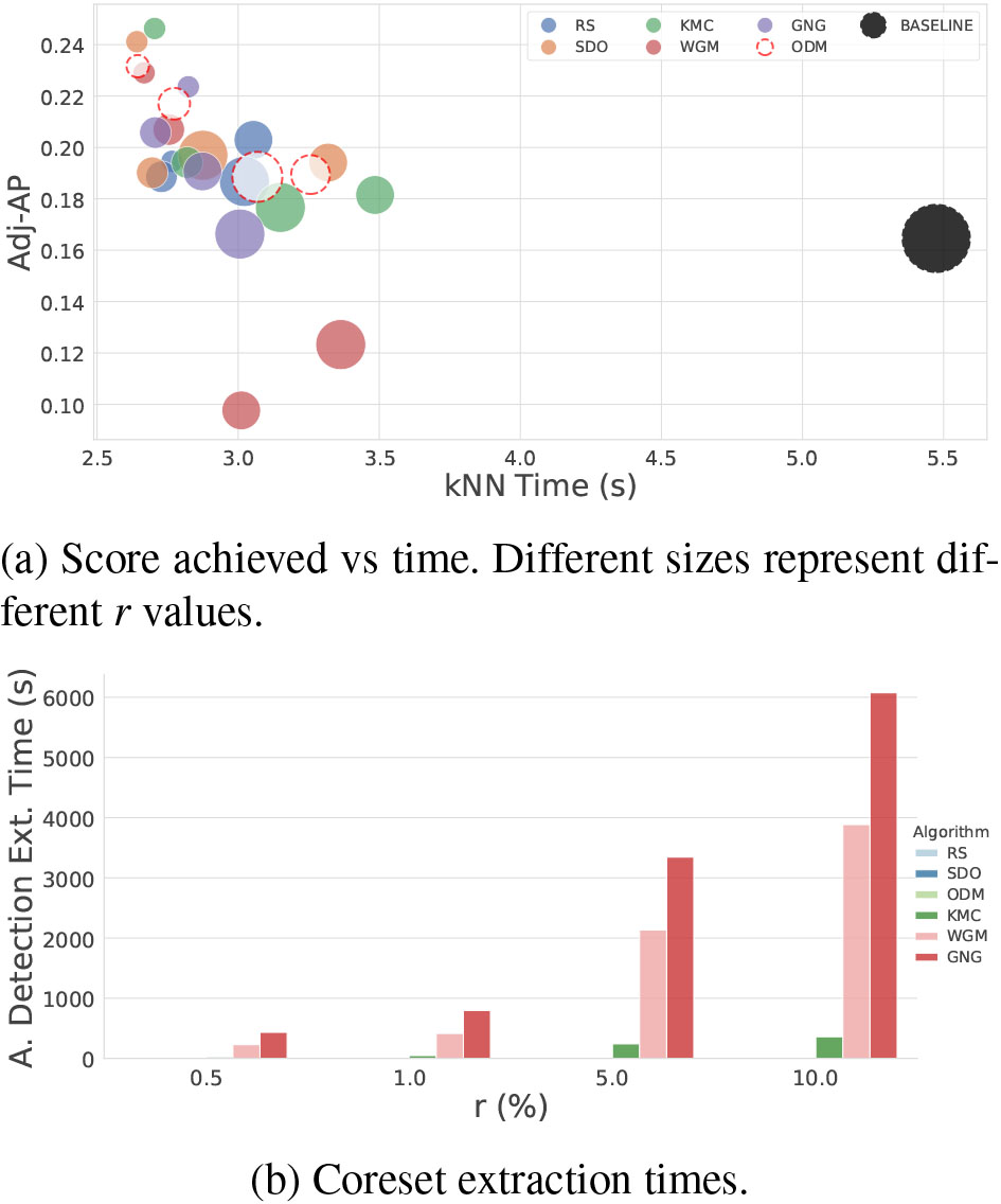

Weighting accuracy and time performances together, only SDO and ODM satisfactorily meet problem requirements. Figure 9a shows a visual comparison of coresets by plotting accuracy (Adjusted Average Precision) versus analysis time (k-NN time). A comparison of coreset extraction times (Ext. Time) is shown in Fig. 9b.

5.2 Clustering

In the clustering experiments (results in Table 4), all tested algorithms show poor performances for very low $r$ (i.e., high dataset summarization). Note that the effect of $r$ is hardly generalizable as it strongly depends on the specific distributions and geometries of the data under analysis. Except for the KMC and WGM algorithms, which obtain low performances even for high $r$ , more quality performances are obtained the more data points we use for the coreset (i.e, higher $r$ ), getting progressively closer to the baseline. SDO and RS obtain almost ideal performances with $r=10\%$ .

Table 4
Clustering performance

Algorithm	r	Adj. rand ind.	Silhouette coeff.	Ext.T.(s)	kM.T.(s)	Lab.E.T.(s)
Baseline	–	0.93 $\pm$ 0.03	0.73 $\pm$ 0.02	–	1.19 $\pm$ 0.04	–
ODM	0.5%	0.66 $\pm$ 0.40	0.52 $\pm$ 0.31	0.14 $\pm$ 0.11	0.73 $\pm$ 0.44	0.09 $\pm$ 0.07
RS		0.51 $\pm$ 0.35	0.44 $\pm$ 0.28	0.00 $\pm$ 0.00	0.74 $\pm$ 0.45	0.09 $\pm$ 0.06
SDO		0.46 $\pm$ 0.34	0.35 $\pm$ 0.27	0.00 $\pm$ 0.00	0.68 $\pm$ 0.49	0.08 $\pm$ 0.07
KMC		0.56 $\pm$ 0.40	0.49 $\pm$ 0.30	0.84 $\pm$ 0.54	0.80 $\pm$ 0.54	0.09 $\pm$ 0.07
WGM		0.59 $\pm$ 0.41	0.51 $\pm$ 0.31	1.58 $\pm$ 2.07	0.78 $\pm$ 0.49	0.09 $\pm$ 0.07
GNG		0.65 $\pm$ 0.40	0.50 $\pm$ 0.31	6.45 $\pm$ 5.47	0.82 $\pm$ 0.53	0.10 $\pm$ 0.08
ODM	1%	0.90 $\pm$ 0.04	0.71 $\pm$ 0.02	0.21 $\pm$ 0.13	1.06 $\pm$ 0.15	0.11 $\pm$ 0.04
RS		0.84 $\pm$ 0.08	0.67 $\pm$ 0.08	0.00 $\pm$ 0.00	1.03 $\pm$ 0.14	0.11 $\pm$ 0.04
SDO		0.75 $\pm$ 0.22	0.59 $\pm$ 0.18	0.01 $\pm$ 0.00	0.95 $\pm$ 0.27	0.11 $\pm$ 0.06
KMC		0.69 $\pm$ 0.21	0.63 $\pm$ 0.08	1.17 $\pm$ 0.26	0.99 $\pm$ 0.09	0.12 $\pm$ 0.06
WGM		0.76 $\pm$ 0.22	0.67 $\pm$ 0.05	2.51 $\pm$ 1.96	1.09 $\pm$ 0.25	0.12 $\pm$ 0.06
GNG		0.88 $\pm$ 0.05	0.70 $\pm$ 0.05	10.13 $\pm$ 6.38	1.12 $\pm$ 0.28	0.11 $\pm$ 0.06
ODM	5%	0.90 $\pm$ 0.06	0.70 $\pm$ 0.06	0.20 $\pm$ 0.10	1.02 $\pm$ 0.07	0.11 $\pm$ 0.04
RS		0.90 $\pm$ 0.05	0.71 $\pm$ 0.03	0.00 $\pm$ 0.00	1.02 $\pm$ 0.07	0.11 $\pm$ 0.03
SDO		0.90 $\pm$ 0.04	0.71 $\pm$ 0.03	0.04 $\pm$ 0.03	1.03 $\pm$ 0.06	0.11 $\pm$ 0.04
KMC		0.68 $\pm$ 0.23	0.59 $\pm$ 0.15	2.02 $\pm$ 1.03	0.99 $\pm$ 0.15	0.11 $\pm$ 0.05
WGM		0.67 $\pm$ 0.24	0.57 $\pm$ 0.19	12.64 $\pm$ 10.52	1.09 $\pm$ 0.18	0.12 $\pm$ 0.05
GNG		0.84 $\pm$ 0.10	0.69 $\pm$ 0.06	23.09 $\pm$ 17.53	1.11 $\pm$ 0.30	0.11 $\pm$ 0.06
ODM	10%	0.89 $\pm$ 0.12	0.70 $\pm$ 0.08	0.19 $\pm$ 0.08	1.01 $\pm$ 0.03	0.11 $\pm$ 0.04
RS		0.92 $\pm$ 0.03	0.72 $\pm$ 0.02	0.00 $\pm$ 0.00	1.00 $\pm$ 0.04	0.11 $\pm$ 0.04
SDO		0.92 $\pm$ 0.03	0.72 $\pm$ 0.02	0.07 $\pm$ 0.05	1.00 $\pm$ 0.03	0.12 $\pm$ 0.05
KMC		0.66 $\pm$ 0.25	0.57 $\pm$ 0.16	3.01 $\pm$ 1.62	0.97 $\pm$ 0.05	0.10 $\pm$ 0.04
WGM		0.57 $\pm$ 0.24	0.50 $\pm$ 0.23	25.30 $\pm$ 18.58	1.03 $\pm$ 0.12	0.11 $\pm$ 0.04
GNG		0.79 $\pm$ 0.21	0.65 $\pm$ 0.11	34.18 $\pm$ 26.41	1.09 $\pm$ 0.22	0.11 $\pm$ 0.06

Ext.T.: Time needed to build a coreset. kM.T.: Time needed to build a kMeans model. Lab.E.T.: Time needed to extend labels.

Figure 10.

Visual representation of the clustering performance.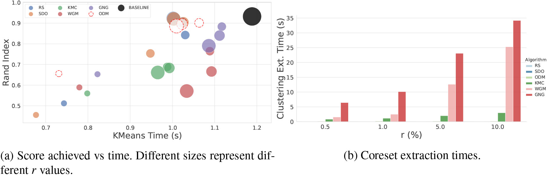

Again, coreset extraction costs (Ext.T.) are considerably high for WGM and GNG. Weighting accuracy and time performances together, the best trade-off is obtained by SDO and ODM, or even RS. Figure 10a shows a scatter plot comparing accuracies (RAND index) vs analysis time (kMeans time). A comparison of coreset extraction times (Ext. Time) is displayed in Fig. 10b.

5.3 Supervised classification

Similarly to the unsupervised classification experiments, in the supervised classification framework higher values of $r$ tend to improve performances and get closer to the baseline (see experiment results in Table 5). The performance reduction when using coresets compared with the baseline case is considerable, but coresets still work satisfactorily if we take into account that they are not dealing with binary classification experiments, but multi-class classification. Best accuracy performances are obtained by ODM, KMC, and RS. Even in spite of the fact that analysis run-times (k-NN time) are not discriminating and more or less equally demanding for all cases, KMC is still a bit slower than other algorithms. On the other hand, if we examine coreset extraction costs (Ext. Time), there are two clearly separable groups: (a) light extraction: RS, SDO, and ODM; and (b) heavy extraction: KMC, WGM, GNG, and CNN. Weighting accuracy and time performances together, ODM and RS offer the best solutions with affordable complexities.

Table 5
Supervised learning performance

Algorithm	r	Accuracy	Mi. Prec.	Ma. Prec.	Mi. Rec.	Ma. Rec.	Ext. Time (s)		k-NN Time (s)
Baseline	–	0.94 $\pm$ 0.09	0.94 $\pm$ 0.09	0.88 $\pm$ 0.09	0.94 $\pm$ 0.09	0.84 $\pm$ 0.10	–		0.29 $\pm$ 0.28
ODM	0.5%	0.85 $\pm$ 0.18	0.85 $\pm$ 0.18	0.56 $\pm$ 0.30	0.85 $\pm$ 0.18	0.56 $\pm$ 0.31	0.63	$\pm$ 0.30	0.12 $\pm$ 0.06
RS		0.83 $\pm$ 0.19	0.83 $\pm$ 0.19	0.60 $\pm$ 0.30	0.83 $\pm$ 0.19	0.52 $\pm$ 0.32	0.00	$\pm$ 0.00	0.12 $\pm$ 0.06
SDO		0.75 $\pm$ 0.24	0.75 $\pm$ 0.24	0.46 $\pm$ 0.29	0.75 $\pm$ 0.24	0.51 $\pm$ 0.33	0.02	$\pm$ 0.01	0.11 $\pm$ 0.05
KMC		0.82 $\pm$ 0.19	0.82 $\pm$ 0.19	0.55 $\pm$ 0.34	0.82 $\pm$ 0.19	0.46 $\pm$ 0.27	4.88	$\pm$ 3.40	0.19 $\pm$ 0.08
WGM		0.65 $\pm$ 0.39	0.65 $\pm$ 0.39	0.54 $\pm$ 0.38	0.65 $\pm$ 0.39	0.45 $\pm$ 0.34	6.52	$\pm$ 7.34	0.09 $\pm$ 0.07
GNG		0.82 $\pm$ 0.19	0.82 $\pm$ 0.19	0.57 $\pm$ 0.32	0.82 $\pm$ 0.19	0.48 $\pm$ 0.25	31.30	$\pm$ 16.28	0.12 $\pm$ 0.06
CNN		0.63 $\pm$ 0.29	0.63 $\pm$ 0.29	0.41 $\pm$ 0.29	0.63 $\pm$ 0.29	0.50 $\pm$ 0.23	65.94	$\pm$ 115.28	0.11 $\pm$ 0.05
ODM	1%	0.88 $\pm$ 0.17	0.88 $\pm$ 0.17	0.63 $\pm$ 0.26	0.88 $\pm$ 0.17	0.59 $\pm$ 0.28	0.73	$\pm$ 0.44	0.14 $\pm$ 0.09
RS		0.85 $\pm$ 0.19	0.85 $\pm$ 0.19	0.62 $\pm$ 0.27	0.85 $\pm$ 0.19	0.56 $\pm$ 0.29	0.01	$\pm$ 0.01	0.14 $\pm$ 0.09
SDO		0.83 $\pm$ 0.24	0.83 $\pm$ 0.24	0.60 $\pm$ 0.29	0.83 $\pm$ 0.24	0.57 $\pm$ 0.30	0.04	$\pm$ 0.02	0.11 $\pm$ 0.05
KMC		0.86 $\pm$ 0.18	0.86 $\pm$ 0.18	0.62 $\pm$ 0.29	0.86 $\pm$ 0.18	0.54 $\pm$ 0.30	5.59	$\pm$ 3.79	0.19 $\pm$ 0.09
WGM		0.67 $\pm$ 0.39	0.67 $\pm$ 0.39	0.54 $\pm$ 0.38	0.67 $\pm$ 0.39	0.50 $\pm$ 0.35	12.16	$\pm$ 13.37	0.10 $\pm$ 0.08
GNG		0.84 $\pm$ 0.17	0.84 $\pm$ 0.17	0.60 $\pm$ 0.30	0.84 $\pm$ 0.17	0.53 $\pm$ 0.25	41.26	$\pm$ 22.74	0.12 $\pm$ 0.06
CNN		0.68 $\pm$ 0.29	0.68 $\pm$ 0.29	0.44 $\pm$ 0.26	0.68 $\pm$ 0.29	0.53 $\pm$ 0.21	66.64	$\pm$ 116.62	0.11 $\pm$ 0.05
ODM	5%	0.90 $\pm$ 0.14	0.90 $\pm$ 0.14	0.67 $\pm$ 0.25	0.90 $\pm$ 0.14	0.62 $\pm$ 0.25	0.64	$\pm$ 0.31	0.14 $\pm$ 0.08
RS		0.89 $\pm$ 0.16	0.89 $\pm$ 0.16	0.75 $\pm$ 0.26	0.89 $\pm$ 0.16	0.62 $\pm$ 0.26	0.00	$\pm$ 0.00	0.14 $\pm$ 0.08
SDO		0.64 $\pm$ 0.37	0.64 $\pm$ 0.37	0.50 $\pm$ 0.41	0.64 $\pm$ 0.37	0.44 $\pm$ 0.32	0.18	$\pm$ 0.14	0.12 $\pm$ 0.06
KMC		0.89 $\pm$ 0.15	0.89 $\pm$ 0.15	0.66 $\pm$ 0.25	0.89 $\pm$ 0.15	0.60 $\pm$ 0.23	10.38	$\pm$ 6.30	0.21 $\pm$ 0.11
WGM		0.63 $\pm$ 0.37	0.63 $\pm$ 0.37	0.53 $\pm$ 0.35	0.63 $\pm$ 0.37	0.56 $\pm$ 0.35	54.34	$\pm$ 58.35	0.11 $\pm$ 0.10
GNG		0.89 $\pm$ 0.13	0.89 $\pm$ 0.13	0.67 $\pm$ 0.25	0.89 $\pm$ 0.13	0.61 $\pm$ 0.25	106.06	$\pm$ 69.87	0.14 $\pm$ 0.08
CNN		0.85 $\pm$ 0.15	0.85 $\pm$ 0.15	0.67 $\pm$ 0.16	0.85 $\pm$ 0.15	0.69 $\pm$ 0.23	66.50	$\pm$ 116.09	0.14 $\pm$ 0.07
ODM	10%	0.91 $\pm$ 0.13	0.91 $\pm$ 0.13	0.78 $\pm$ 0.24	0.91 $\pm$ 0.13	0.64 $\pm$ 0.24	0.65	$\pm$ 0.31	0.16 $\pm$ 0.10
RS		0.90 $\pm$ 0.15	0.90 $\pm$ 0.15	0.77 $\pm$ 0.23	0.90 $\pm$ 0.15	0.64 $\pm$ 0.25	0.00	$\pm$ 0.00	0.15 $\pm$ 0.09
SDO		0.63 $\pm$ 0.36	0.63 $\pm$ 0.36	0.54 $\pm$ 0.35	0.63 $\pm$ 0.36	0.49 $\pm$ 0.30	0.38	$\pm$ 0.30	0.14 $\pm$ 0.08
KMC		0.90 $\pm$ 0.13	0.90 $\pm$ 0.13	0.77 $\pm$ 0.25	0.90 $\pm$ 0.13	0.61 $\pm$ 0.22	14.65	$\pm$ 8.91	0.23 $\pm$ 0.13
WGM		0.60 $\pm$ 0.36	0.60 $\pm$ 0.36	0.53 $\pm$ 0.34	0.60 $\pm$ 0.36	0.57 $\pm$ 0.35	104.27	$\pm$ 112.55	0.13 $\pm$ 0.12
GNG		0.91 $\pm$ 0.13	0.91 $\pm$ 0.13	0.76 $\pm$ 0.25	0.91 $\pm$ 0.13	0.63 $\pm$ 0.21	173.76	$\pm$ 122.99	0.16 $\pm$ 0.10
CNN		0.75 $\pm$ 0.30	0.75 $\pm$ 0.30	0.55 $\pm$ 0.27	0.75 $\pm$ 0.30	0.63 $\pm$ 0.22	66.16	$\pm$ 115.79	0.15 $\pm$ 0.09

Ext.T.: Time needed to build a coreset. Ma.: Macro. Mi.: Micro.

Figure 11.

Visual representation of the supervised learning performance.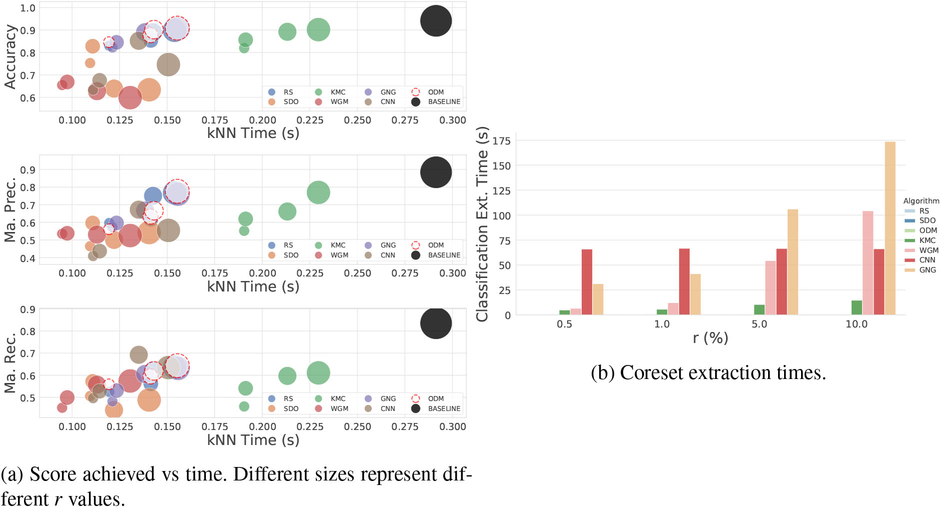

The CNN additionally appears in this set of experiments as it was specifically proposed for alleviating the computational costs of k-nn-based classification. However, it is a heavy algorithm in terms of extraction costs when compared to ODM or SDO, and accuracy performances are in line or below most of the competitors. Note that, in its original implementation, CNN automatically establishes the size of the coreset according to dataset properties and cannot be externally implemented. This fact might be affecting its capability of obtaining better performances.

Alike previous experiments, Fig. 11a compares coresets by using classification metrics (Accuracy, Macro Precision, Macro Recall) vs analysis time (kNN time). A comparison of coreset extraction times (Ext. Time) is displayed in Fig. 11b.

5.4 Results overview

Figure 12.

Critical Difference Diagrams. The methods are ordered in such a way that the best one is the rightmost one. Methods whose difference is not shown to be significant in the tests are joined with a thick line.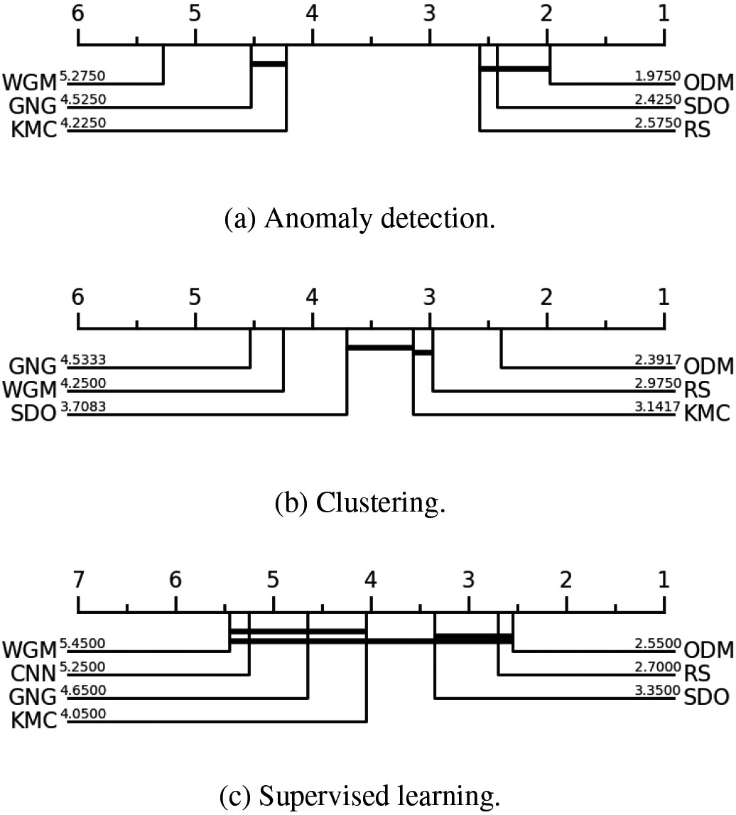

Evaluating all experiments together, ODM stands out as it is the only particularly stable method (i.e, its performance are among the top ones regardless of the application) and keeps considerable low time-complexity costs.

To confirm statistically significant differences among the coreset extractor methodologies under test, we used Critical Difference Diagrams (CDD) [19, 30], which are based on the Wilcoxon signed-rank test [44]. Figure 12 show CDD for the three experimental applications: anomaly detection, clustering, and supervised classification. For the calculation of CDD, we combined all metrics shown in Tables 3–5 after z-scoring them to make them comparable and addable. Thus, we obtained one summary metric for each experimental application. In CDD methods are ordered to keep the best ones on the right side of the diagram. Methods whose different performances are not deemed significant are joined by thick horizontal lines. CDD confirm the preponderance of ODM over competitors regardless of application, followed by RS and SDO.

6. Conclusion

We have presented ODM, a lightweight algorithm for the extraction of low-density data models (data summaries, coresets) in log-linear times. We have tested ODM and compared it with state-of-the-art alternatives by using multiple datasets in fundamental machine learning areas, namely: anomaly detection, clustering, and supervised classification. Obtained results place ODM as the most stable option and the best trade-off between time-complexity and performance accuracy. ODM is strongly recommended for alleviating computational demands when facing the analysis of large datasets. Future research includes: using ODM as an under-sampling method for applications where classes show strong imbalance (e.g., attack detection in network traffic); applying ODM for streaming data, where it is necessary to keep a model of the data up to date (therefore, able to evolve), but, at the same time, preventing that the accumulation of new samples deteriorate the model in use. Finally, also concerning streaming applications, evaluate the potential of ODM to discover emerging clusters and differentiate them quickly and efficiently from simple anomalies.

References

Abe

Zadrozny

and Langford

, Outlier detection by active learning, in: Proceedings of the 12th ACM SIGKDD International Conference on Knowledge Discovery and Data Mining, ACM, 2006, pp. 504–509.

Agarwal

P.K.

Har-Peled

and Varadarajan

K.R.

, Geometric approximation via coresets, Combinatorial and Computational Geometry 52 (2005), 1–30.

Aggarwal

Hinneburg

and Keim

D.A.

, On the surprising behavior of distance metrics in high dimensional space, in: International Conference on Database Theory, Springer, 2001, pp. 420–434.

Angiulli

, Fast condensed nearest neighbor rule, in: Proceedings of the 22nd International Conference on Machine Learning, 2005, pp. 25–32.

Arthur

and Vassilvitskii

, k-means++: The advantages of careful seeding, Technical report, Stanford, 2006.

Attias

, A variational baysian framework for graphical models, in: Advances in Neural Information Processing Systems, 2000, pp. 209–215.

Bachem

Lucic

and Krause

, Scalable k-means clustering via lightweight coresets, in: Proceedings of the 24th ACM SIGKDD International Conference on Knowledge Discovery & Data Mining, 2018, pp. 1119–1127.

Bentley

J.L.

, Multidimensional binary search trees used for associative searching, Communications of the ACM 18(9) (1975), 509–517.

Blackard

J.A.

and Dean

D.J.

, Comparative accuracies of artificial neural networks and discriminant analysis in predicting forest cover types from cartographic variables, Computers and Electronics in Agriculture 24(3) (1999), 131–151.

10.

Campbell

and Beronov

, Sparse variational inference: Bayesian coresets from scratch, arXiv preprint arXiv:1906.03329, 2019.

11.

Campbell

and Broderick

, Bayesian coreset construction via greedy iterative geodesic ascent, arXiv preprint arXiv:1802.01737, 2018.

12.

Campbell

and Broderick

, Automated scalable bayesian inference via hilbert coresets, The Journal of Machine Learning Research 20(1) (2019), 551–588.

13.

Campos

G.O.

Zimek

Sander

Campello

R.J.

Micenková

Schubert

Assent

and Houle

M.E.

, On the evaluation of unsupervised outlier detection: Measures, datasets, and an empirical study, Data Mining and Knowledge Discovery 30(4) (2016), 891–927.

14.

Candanedo

L.M.

and Feldheim

, Accurate occupancy detection of an office room from light, temperature, humidity and co2 measurements using statistical learning models, Energy and Buildings 112 (2016), 28–39.

15.

Ciaccia

Patella

and Zezula

, M-tree: An e cient access method for similarity search in metric spaces, in: Proceedings of the 23rd VLDB Conference, Athens, Greece, Citeseer, 1997, pp. 426–435.

16.

Cortez

Cerdeira

Almeida

Matos

and Reis

, Modeling wine preferences by data mining from physicochemical properties, Decision Support Systems 47(4) (2009), 547–553.

17.

data

, mopsi-finland, url = https://github.com/deric/clustering-benchmark/blob/master/src/main/resources/datasets/artificial/mopsi-finland.arff, urldate = 2019-08-19.

18.

De Stefano

Maniaci

Fontanella

and di Freca

A.S.

, Reliable writer identification in medieval manuscripts through page layout features: The “avila” bible case, Engineering Applications of Artificial Intelligence 72 (2018), 99–110.

19.

Demšar

, Statistical comparisons of classifiers over multiple data sets, The Journal of Machine Learning Research 7 (2006), 1–30.

20.

Evett

I.W.

and Spiehler

E.J.

, Rule induction in forensic science, KBS in Goverment, 1987, 107–118.

21.

Feldman

Schmidt

and Sohler

, Turning big data into tiny data: Constant-size coresets for k-means, pca, and projective clustering, SIAM Journal on Computing 49(3) (2020), 601–657.

22.

Fränti

Mariescu-Istodor

and Zhong

, Xnn graph, in: Joint IAPR International Workshops on Statistical Techniques in Pattern Recognition (SPR) and Structural and Syntactic Pattern Recognition (SSPR), Springer, 2016, pp. 207–217.

23.

Fränti

Rezaei

and Zhao

, Centroid index: Cluster level similarity measure, Pattern Recognition 47(9) (2014), 3034–3045.

24.

Fritzke

, A growing neural gas network learns topologies, in: Advances in Neural Information Processing Systems, 1995, pp. 625–632.

25.

Geusebroek

J.-M.

Burghouts

G.J.

and Smeulders

A.W.

, The amsterdam library of object images, International Journal of Computer Vision 61(1) (2005), 103–112.

26.

Hart

, The condensed nearest neighbor rule (corresp.), IEEE Transactions on Information Theory 14(3) (1968), 515–516.

27.

Hubert

and Arabie

, Comparing partitions, Journal of Classification 2(1) (1985), 193–218.

28.

Huggins

Campbell

and Broderick

, Coresets for scalable bayesian logistic regression, in: Advances in Neural Information Processing Systems, 2016, pp. 4080–4088.

29.

Iglesias

Zseby

Ferreira

and Zimek

, Mdcgen: Multidimensional dataset generator for clustering, Journal of Classification, 1–20.

30.

Ismail Fawaz

Forestier

Weber

Idoumghar

and Muller

P.-A.

, Deep learning for time series classification: A review, Data Mining and Knowledge Discovery 33(4) (2019), 917–963.

31.

Johnson

B.A.

Tateishi

and Hoan

N.T.

, A hybrid pansharpening approach and multiscale object-based image analysis for mapping diseased pine and oak trees, International Journal of Remote Sensing 34(20) (2013), 6969–6982.

32.

Kärkkäinen

and Fränti

, Dynamic Local Search Algorithm for the Clustering Problem, University of Joensuu, 2002.

33.

Keith

Jameson

Van Straten

Bailes

Johnston

Kramer

Possenti

Bates

Bhat

Burgay

et al., The high time resolution universe pulsar survey – i. system configuration and initial discoveries, Monthly Notices of the Royal Astronomical Society 409(2) (2010), 619–627.

34.

Keller

Muller

and Bohm

, Hics: High contrast subspaces for density-based outlier ranking, in: 2012 IEEE 28th International Conference on Data Engineering, IEEE, 2012, pp. 1037–1048.

35.

Kohonen

, The self-organizing map, Proceedings of the IEEE 78(9) (1990), 1464–1480.

36.

Lucic

Faulkner

Krause

and Feldman

, Training gaussian mixture models at scale via coresets, The Journal of Machine Learning Research, 2017, 5885–5909.

37.

Martinetz

Schulten

et al., A “neural-gas” network learns topologies, 1991.

38.

Mirzasoleiman

Bilmes

and Leskovec

, Coresets for data-efficient training of machine learning models, in: International Conference on Machine Learning, PMLR, 2020, pp. 6950–6960.

39.

Ramaswamy

Rastogi

and Shim

, Efficient algorithms for mining outliers from large data sets, in: Proceedings of the 2000 ACM SIGMOD International Conference on Management of Data, 2000, pp. 427–438.

40.

Rezaei

and Fränti

, Set matching measures for external cluster validity, IEEE Transactions on Knowledge and Data Engineering 28(8) (2016), 2173–2186.

41.

Rousseeuw

P.J.

, Silhouettes: A graphical aid to the interpretation and validation of cluster analysis, Journal of Computational and Applied Mathematics 20 (1987), 53–65.

42.

Ultsch

, Clustering with som: U^* c, in: Proceedings of the Workshop on Self-organizing Maps, 2005, 2005.

43.

Vázquez

F.I.

Zseby

and Zimek

, Outlier detection based on low density models, in: 2018 IEEE International Conference on Data Mining Workshops (ICDMW), 2018, pp. 970–979.

44.

Wilcoxon

, Individual comparisons by ranking methods, in: Breakthroughs in Statistics, Springer, 1992, pp. 196–202.

45.

Yamanishi

Takeuchi

J.-I.

Williams

and Milne

, On-line unsupervised outlier detection using finite mixtures with discounting learning algorithms, Data Mining and Knowledge Discovery 8(3) (2004), 275–300.

46.

Zimek

Gaudet

Campello

R.J.

and Sander

, Subsampling for efficient and effective unsupervised outlier detection ensembles, in: Proceedings of the 19th ACM SIGKDD International Conference on Knowledge Discovery and Data Mining, 2013, pp. 428–436.

Modeling data with observers

Abstract

Keywords

1. Introduction

2. Related work

2.1 Statistics and error optimization

2.2 Distance-based methods

2.3 Neural networks

3. ODM

1 github.com/CN-TU/pyodm.

3.2 Algorithm

5.1 Anomaly detection

Table 3 Performance of detecting anomalies

Table 4 Clustering performance

Table 5 Supervised learning performance

References

¹
github.com/CN-TU/pyodm.

Table 3
Performance of detecting anomalies

Table 4
Clustering performance

Table 5
Supervised learning performance