Stock market network based on bi-dimensional histogram and autoencoder

Abstract

In this study, we propose a deep learning related framework to analyze S&P500 stocks using bi-dimensional histogram and autoencoder. The bi-dimensional histogram consisting of daily returns of stock price and stock trading volume is plotted for each stock. Autoencoder is applied to the bi-dimensional histogram to reduce data dimension and extract meaningful features of a stock. The histogram distance matrix for stocks are made of the extracted features of stocks, and stock market network is built by applying Planar Maximally Filtered Graph(PMFG) algorithm to the histogram distance matrix. The constructed stock market network represents the latent space of bi-dimensional histogram, and network analysis is performed to investigate the structural properties of the stock market. we discover that the structural properties of stock market network are related to the dispersion of bi-dimensional histogram. Also, we confirm that the autoencoder is effective in extracting the latent feature of the bi-dimensional histogram. Portfolios using the features of bi-dimensional histogram network are constructed and their investment performance is evaluated in comparison with other benchmark portfolios. We observe that the portfolio consisting of stocks corresponding to the peripheral nodes of bi-dimensional histogram network shows better investment performance than other benchmark stock portfolios.

Keywords

Autoencoder complex network dimensionality reduction latent space visualization histogram stock portfolio

1. Introduction

Stock markets which fluctuate chaotically are modelled as complex networks formed through the interaction of individual factors [35]. Many studies have used network analysis to investigate the relationship between stocks [35, 53, 34, 20, 11, 23, 42, 19, 41, 40, 28, 16, 44, 29, 57, 26, 6, 24, 51, 52, 17, 13, 49, 37, 38]. Mantegna [34] analyzed stock markets through Minimum Spanning Tree (MST) network for the first time, observing the structure of Dow Jones stock market. MST is a filtered graph connecting all the $N$ nodes of the graph with $N-1$ edges so that the sum of edge distance is minimum [42]. In this way, MST extracts the most important information in graph [26]. Many studies have used MST to investigate the structural information inherent in financial stock prices [42, 6, 24]. Tumminello et al. [51] applied Planar Maximally Filtered Graph (PMFG) to construct a stock market network in order to preserve more information on the relationship between stocks. In [51], Tumminello et al. studied the topological properties of a PMFG constructed from the top 300 companies of the New York Stock Exchange (NYSE) during 2001–2003, verifying that loops and cliques in PMFG have the important relationship with the market properties. PMFG contains more stock market information than MST by allowing loops and cliques as well as preserves the hierarchical structure of the MST. Also, PMFG of stock market provide a stronger robustness and dynamical stability than MST of stock market [13]. Based on these properties, PMFG has been used in stock market analysis [51, 52, 17, 13, 49, 37, 38, 57], clustering [50, 37] and investment applications [44, 58, 59, 31, 29].

In defining interactions between stocks, many studies highlighted stock price time series. However, information on stocks is not only contained in the price, but also in various data such as trading volumes, volatility and accounting variables. In particular, we focus on trading volumes of stocks in addition to their prices. From a practical point of view, trading volumes have much significant information. For example, the increment of trading volume at the floor of stock price is regarded as a signal of upward conversion. Conversely, the decrement of trading volume at the ceiling of stock price is understood as a signal of a downward turn. As such, the trading volume could indicate the direction of stock price. Also, stock return and trading volume interact with each other in the stock market dynamics [27]. Various studies have been conducted to analyze the properties contained in trading volume and its relationship with stock price. As in stock prices, trading volume has multifractal behavior characteristics [3] and auto-correlation patterns [47]. Lee and Swaminathan [27] revealed that the trend of trading volume is related to the persistence of price momentum and magnitude. Chen et al. [7] confirmed that positive correlation exists between the trading volume and the absolute value of stock price return. Various studies have used the stock price and trading volume together to predict the stock price [55, 54, 9, 14, 33]. The positive correlation between the negative skewness of stock price returns and trading volume was verified through previous studies [15, 8]. Trading volume is correlated with the volatility of stock returns, return on equity (ROE) and return on investment (ROI) [45, 18, 12, 46, 22]. Bajo [4] revealed that the trading volume is an efficient proxy of stock information for market participants.

As described above, the trading volume is important to explain the properties of a stock and the stock market in addition to stock price. Our study attempts to analyze the stock market by considering both stock prices and stock trading volumes. Both of stock price and stock trading volume can be analyzed from a multivariate perspective through the RV coefficient, which is a multivariate generalization of the squared Pearson correlation coefficient. However, the RV coefficient has some drawbacks of difficulty in understanding and high computational cost [25]. In this study, we utilize a bi-dimensional histogram to intuitively represent stock trading volume information as well as stock price information.

As the size of bi-dimensional histogram is relatively large, we apply autoencoder to the bi-dimensional histogram for the latent feature extraction from the reduced bi-dimensional histogram data. Autoencoder (AE) is widely used for feature extraction as a method of deep learning [39, 10, 56, 2, 32, 30, 5, 36, 21]. AE, which consists of two neural networks called encoder and decoder, is a nonlinear dimension reduction methodology and an effective method for manifold learning. AE compresses and reproduces data through an encoder and decoder, and effectively extracts the features inherent in the data.

Based on the extracted features, we build the bi-dimensional histogram network of the stock market using the PMFG algorithm, and network analysis is performed to investigate the structural properties of the stock market. The novelty of our research is that we construct a stock market PMFG network using the latent features from autoencoder transformed information of bi-dimensional histogram based on stock prices and trading volumes.

The bi-dimensional histogram network is applied to construct stock investment portfolio. There are many studies incorporating the network topological property into the construction of stock portfolio [44, 58, 59, 31, 29]. Pozzi et al. [44] proposed a measure to quantify the level of the network periphery, and showed that the portfolio of stocks in the periphery of network performs better than that of stocks in the center of network. Based on this property, we investigate the usefulness of a histogram network in terms of portfolio selection.

The paper is organized as follows. Section 2 reviews previous studies of the stock market network, as well as studies of autoencoder in the stock market. Section 3 describes the data, bi-dimensional histogram, autoencoder, stock network, and portfolio application. Section 4 presents the result of our suggested method including the features of bi-dimensional histogram and network analysis. Finally, the summary of our research is provided in Section 5.

2. Related work

2.1 Stock market network

In econophysics, the stock market network plays an important role in analyzing the characteristics of financial markets. After Mantegna’s research [34], which first introduced the network concept through MST to analyze the stock market, many studies have used MST to analyze financial markets. Onnela et al. [42] constructed MST network of S&P500 stocks to study the dynamics of the stock market, finding that normalized tree length of the MST decreases and remains low during the financial crisis. Bonanno et al. [6] revealed that the MST of the stock market has a structured hierarchy. Jung et al. [24] studied the MST of the Korean stock market and found that the characteristics of the Korean stock market differ from that of the US market. However, the drawback of MST is that valuable information about the relationship between stocks is necessarily lost. To complement the drawback of MST, Tumminello et al. [51] proposed a stock market network using PMFG. PMFG is a graph using the planarity property, and loops and cliques are allowed, including MST in the graph. Various studies have demonstrated that PMFG has a more significant and richer structure, stronger robustness, and better dynamical stability than MST [51, 43, 13]. PMFG is a conventional method to build a stock market network and is used in various fields. Zhang and Zhuang [57] built a Chinese stock market network using PMFG and investigated the relationship between network stability and stock market volatility. Musmeci et al. [38] analyzed the NYSE stock market with PMFG. Musmeci et al.[38] investigated meaningful relationships between past changes in the network structure and future changes in the market volatility. Song et al. [50] confirmed that PMFG effectively extracts clusters and hierarchies from complex data sets. Lu et al. [31] proved that PMFG is also useful in portfolio investment.

2.2 Autoencoder in the stock market

In this study, we propose a framework for constructing a stock market network from a multivariate perspective using autoencoder and PMFG. As the dimension of the variable increases, the higher dimension variable can lead to redundancy of information and reduce the efficiency and accuracy of algorithms. In this context, autoencoder, a deep learning model, is a method that extracts meaningful features from high-dimensional variables and is also in the spotlight in the finance domain. Lv et al. [32] performed feature extraction of 44 technical indicators for stock using autoencoder and applied it to predicting trading signals. Bao et al. [5] extracted features by compressing daily trading data, technical indicators, and macroeconomic variables with an autoencoder. And [5] verified the usefulness of autoencoder by using compressed features for stock price prediction. Moews and Ibikunle [36] extracted latent features of high-frequency transaction data using autoencoder and used it for stock price movement prediction. Moews and Ibikunle [36] also demonstrated that this approach works even in highly volatile market conditions such as the financial crisis. Huh [21] applied autoencoder to predict the systematic risk of the stock market. In previous studies using autoencoder in the finance domain, features extracted through autoencoder are mainly used for prediction. In this study, we focus on structuring the stock market using features extracted through autoencoder. We transform the stock price and trading volume into a bi-dimensional histogram and perform feature extraction through an autoencoder. Then, we build a stock market network by applying the PMFG algorithm to the latent space of the extracted features. To the best of our knowledge, our approach is the first attempt to use the bi-dimensional histogram and autoencoder to construct the stock market network. Based on the stock market network constructed by our method, we perform network analysis to investigate the structural properties of the stock market. And we utilize the stock market network to construct a stock investment portfolio.

3. Data and methods

The data in this study is comprised of the daily adjusted stock prices and daily trading volumes of stocks included in S&P500 from January 3, 2006 to September 30, 2019, which amount to 3459 data points. Among the stocks that have been listed in S&P500 over the entire period, the top 400 stocks are selected on the market cap basis. The description of the stocks is provided in appendix. Table 1 is the result of classifying the stocks into 11 sectors according to the Global Industry Classification Standard (GICS) industry category system. Stocks are classified into 11 sectors, Financials (FINC), Industrials (INDS), Consumer Discretionary (COND), Information Technology (INFT), Health Care (HLCA), Consumer Staples (CONS), Real Estate (REES), Utilities (UTIL), Energy (ENRG), Material (MTRS), and Communication Services (CONS). The largest and the smallest industry sectors are the financial sector and the Communicaion Services sector, accounting for 59 stocks (14.75%) and 14 stocks (3.5%), respectively.

Table 1
Summary of GICS industry classification of stocks

Sector	Number of stocks	Percentage	Sector	Number of stocks	Percentage	Sector	Number of stocks	Percentage
FINC	59	14.75%	HLCA	49	12.25%	ENRG	22	5.50%
INDS	52	13.00%	CONS	29	7.25%	MTRS	21	5.25%
COND	50	12.50%	REES	28	7.00%	CONS	14	3.50%
INFT	49	12.25%	UTIL	27	6.75%

3.1 Bi-dimensional histogram

Bi-dimensional histogram maps pairs of two variables to bi-dimensional grid bins. Given the number of all observation pairs, $M$ , and the number of bins for the first and the second variables, $m_{1}$ and $m_{2}$ , respectively, frequency $h_{k,j}$ satisfies the following condition.

$\displaystyle M=\sum_{k=1}^{m_{1}}\sum_{j=1}^{m_{2}}h_{k,j}$ (1)

When denoting the closing price of $i$ th stock at time $t$ as $C_{i}(t)$ , the corresponding price return is $RC_{i}(t)=\text{ln}(C_{i}(t)/C_{i}(t-1))$ . Likewise, the return of the trading volume of $i$ th stock is $RV_{i}(t)=\text{ln}(V_{i}(t)/V_{i}(t-1))$ where $V_{i}(t)$ is the trading volume at the time $t$ . The observation pair of $i$ th stock at time $t$ is $(RC_{i}(t),RV_{i}(t))$ . We consider 400 stocks in S&P 500 so that stock index $i$ varies from 1 to 400. In the consideration of auto-encoder model structure and time complexity of the learning process, the range of axes for the price and trading volume returns is set to 99% quantile as upper limit and 1% quantile as lower limit. The values outside the range are set to the either limit. Then, the interval between lower limit and upper limit is divided into 11 bins. In this way, price and trading volume returns are set to 11 categories respectively for bi-dimensional histogram bin. This implies that both $m_{1}$ and $m_{2}$ in Eq. (1) set to 11.

Based on the bin size set above, $(RC_{i}(t),RV_{i}(t))$ is mapped to 121 bi-dimensional bins. Each observation period is the time window of 250 trading days implying that the total number of frequencies, $M$ , in Eq. (1) is 250. The observation period moves by 10 trading days interval from January 3, 2006 to September 30, 2019, and the total number of observation periods is 321.

Figure 1.

Bi-dimensional histograms of AAPL, ETN and PG.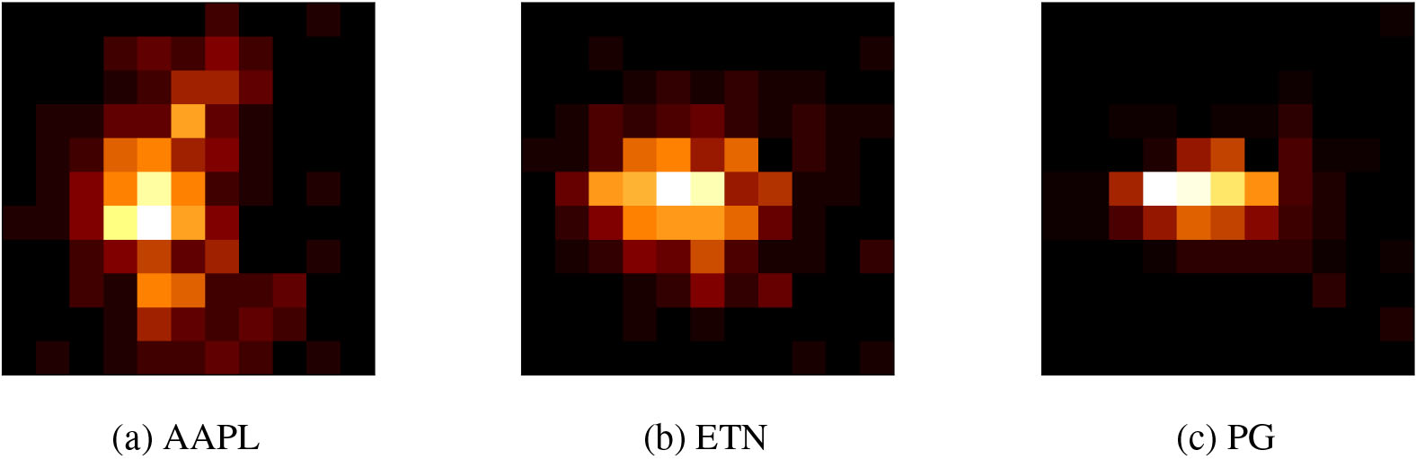

Figure 1 shows bi-dimensional histograms of AAPL, ETN and PG for the first observation period. We define dispersion $v_{H}$ in Eq. (2) to reflect distinct features of each bi-dimensional histogram. The dispersion of histogram is different depending on the stock.

$\displaystyle v_{H}=\sigma_{H_{X}}\cdot\sigma_{H_{Y}}$ (2)

where $\sigma_{H_{X}}$ and $\sigma_{H_{Y}}$ are standard deviations of the bi-dimensional histogram marginal distribution on the X and Y axes, respectively. Figure 2 shows 100 bi-dimensional histograms sorted in the ascending order of $v_{H}$ value at three random time points.

Figure 2.

Bi-dimensional histograms sorted in ascending order of 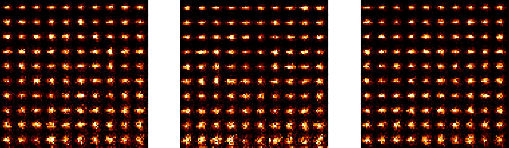$v_{H}$ value.

3.2 Auto-encoder

The main purpose of autoencoder (AE) in deep learning is to learn representation in a data set through unsupervised learning. This representation of the input data is depicted as an internal (hidden) layer or latent vector. AE consists of two parts: encoder and decoder. Encoder compresses input to the lower dimensional latent space. Conversely, decoder reconstructs the input. Through the compression and reconstruction process, most relevant aspects of data are contained in the latent space of the AE.

When denoting the input space as $\mathcal{X}$ , the latent vector space as $\mathcal{F}$ , and the encoder and decoder transitions as $\Phi$ and $\Psi$ respectively, the basic architecture of AE is as follows:

$\displaystyle\Phi:\mathcal{X}\rightarrow\mathcal{F},$ $\displaystyle\Psi:\mathcal{F}\rightarrow\mathcal{X},$ (3) $\displaystyle\phi,\psi\Leftarrow\underset{\Phi,\Psi}{\textrm{argmin}}\;\text{L% }(\mathcal{X},(\Psi\circ\Phi)\mathcal{X}),$

where L is a loss function. As the dimension of $\mathcal{F}$ is lower than that of $\mathcal{X}$ , the latent vector $\Phi(x)$ for $x\in\mathcal{X}$ is the compressed representation of $x$ .

The purpose of the AE in this paper is to learn a bi-dimensional histogram as an input to obtain a latent vector that is a compressed representation of the histogram. The encoder and decoder of the AE are composed of four stages fully connected hidden layers and formulas of the encoder and decoder for the set of parameters ${\Theta}=\{W_{e}^{(k)},W_{d}^{(k)},b_{e}^{(k)},b_{d}^{(k)}|k\in{1,2,3,4}\}$ are as follows. For $k=1,2,3,4$ ,

$\displaystyle x_{e}^{(k)}=\phi^{(k)}(x_{e}^{(k-1)})=a_{e}^{(k)}(W_{e}^{(k)}x_{% e}^{(k-1)}+b_{e}^{(k)}),$ (4) $\displaystyle x_{d}^{(k)}=\psi^{(k)}(x_{d}^{(k-1)})=a_{d}^{(k)}(W_{d}^{(k)}x_{% d}^{(k-1)}+b_{d}^{(k)})$ (5)

where $\phi^{(k)}(\cdot),\psi^{(k)}(\cdot)$ are $k$ th encoding and decoding functions, and $a_{e}^{(k)}(\cdot),a_{d}^{(k)}(\cdot)$ are $k$ th activation functions for encoding and decoding respectively. The weight matrices and bias vectors of the $k$ th encoding and decoding layers are $W_{e}^{(k)},W_{d}^{(k)}$ and $b_{e}^{(k)},b_{d}^{(k)}$ . The input $x\in\mathbb{R}^{121}$ from 11 by 11 bi-dimensional histogram is set as $x_{e}^{(0)}=x$ and $x_{d}^{(0)}=x_{e}^{(4)}$ . We use the ReLU funcion for activation functions except for $a_{d}^{(4)}(\cdot)$ to prevent vanishing gradient phenomenon. For $a_{d}^{(4)}(\cdot)$ , the sigmoid function is used to make $x_{d}^{(4)}$ a value from 0 to 1.

We select the set of parameters $\Theta$ that minimizes the cross-entropy loss function of reconstruction, $\sum_{x\in D}L(x,\hat{x})=-\sum_{x\in D}\big{(}x\text{ln}\hat{x}+(1-x)\text{ln% }(1-\hat{x})\big{)}$ where $D$ is the training data set. Note that $x$ is a vector whose 121 elements belong to the range of $[0,1]$ and $\hat{x}$ is a reconstruction of original input $x$ , $\hat{x}=x_{d}^{(4)}$ .

Table 2 summarizes the dimensions of each layer constituting the AE model, and Fig. 3 is a schematic diagram of the autoencoder structure described in Table 2.

Table 2

Dimensions of weight and bias of hidden layers in autoencoder

	Encoder				Decoder
Layer	1	2	3	4	1	2	3	4
Weight	121 $\times$ 256	256 $\times$ 128	128 $\times$ 64	64 $\times$ 32	32 $\times$ 64	64 $\times$ 128	128 $\times$ 256	256 $\times$ 121
Bias	256	128	64	32	64	128	256	121

In this paper, the learning of AE is conducted on a bi-dimensional histogram. For each of 321 observation period, an AE model corresponding to the period is made. However, training a model using only 400 bi-dimensional histograms can cause over-fitting problems. To prevent this, augmentation is performed during data set construction. In each observation period, gaussian noises are added to price and volume series, and bi-dimensional histograms are constructed from the noisy series. For each stock, augmentation is performed 100 times using gaussian noise, and as a result, 40,000 bi-dimensional histograms are revised in the existing data set. We randomly select 80% of the data set for training and 20% for validation. In the training process, the dimension of the latent vector is set to 32 as above which the validation error does not significantly decrease. Also, the model training process proceeds to 250 epochs because the validation error tends to converge at the epoch. Table 3 compares the reconstruction errors between AE and Principal Component Analysis (PCA) which is a conventional method for dimensionality reduction. Reconstruction error is determined as mean squared error (MSE) between the original data and reconstructed data from the model. In our result, AE shows the better performance than PCA in terms of MSE.

Table 3

Reconstruction error for different algorithms

	AE	PCA	PCA rbf kernel	PCA sigmoid kernel
Mean	6.46E-06	1.41E-05	1.06E-05	2.18E-05
Std	1.26E-06	1.06E-06	6.71E-07	5.08E-07
Max	1.13E-05	1.68E-05	1.23E-05	2.34E-05
Min	3.30E-06	1.07E-05	8.66E-06	2.08E-05
$p$ -value		1.99E-238	2.83E-172	0.00E+00

${}^{*}$ Note: $p$ -value refers to the statistical significance of the paired $t$ -test result in comparison with AE.

Figure 3.

Structure of autoencoder for feature extraction from bi-dimensional histogram.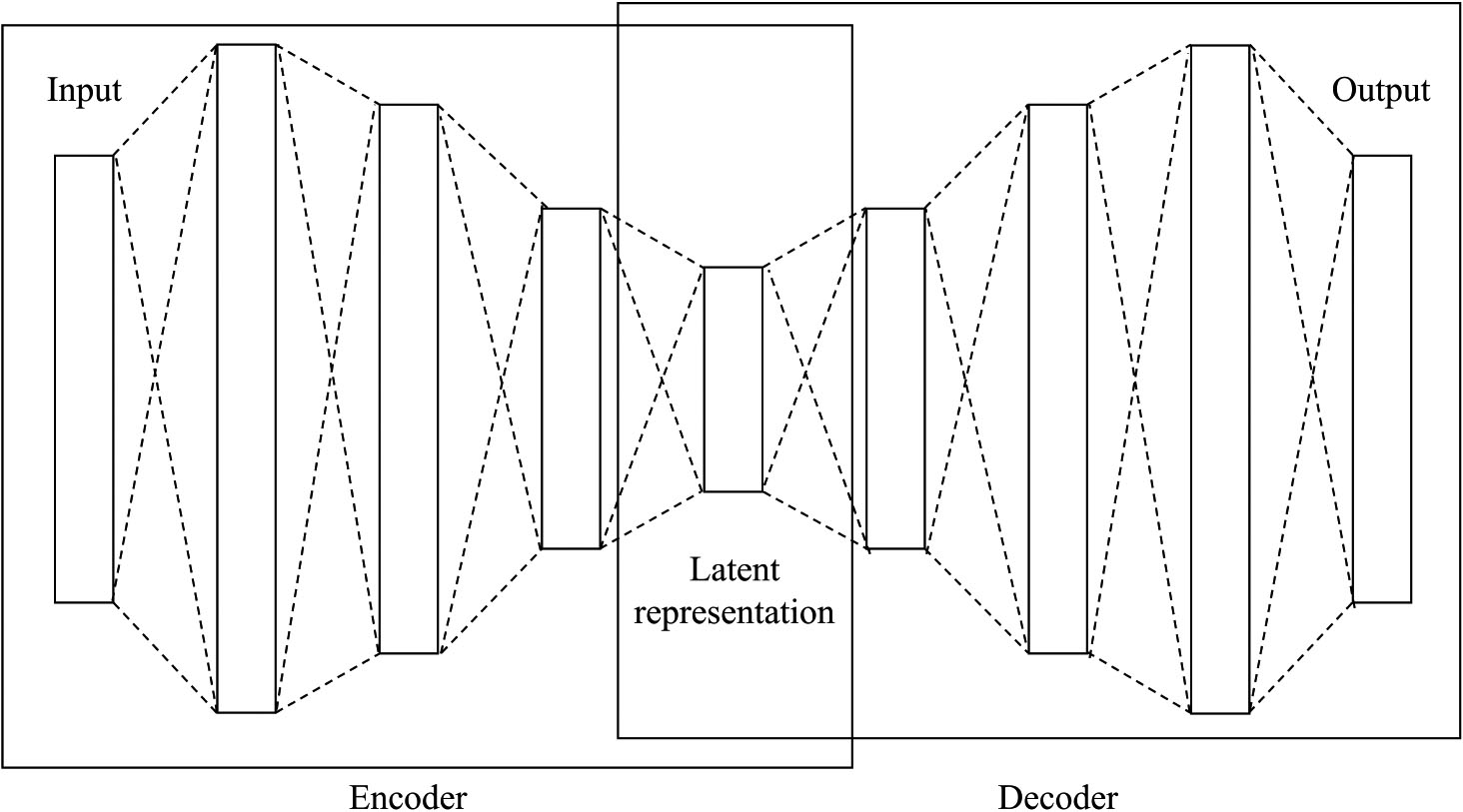

3.3 Stock market network analysis

We transform the bi-dimensional histogram of each stock into a latent vector through the encoder. In each observation period, the latent vector of the $i$ th stock is a 32-dimensional vector in the form of $LV_{i}=(\ell v_{i,1},\ldots,\ell v_{i,32})$ . This is a compressed feature vector of a bi-dimensional histogram, which corresponds to $x_{d}^{(4)}$ in Eq. (5). We calculate the euclidian distance between stocks based on the latent vector and the formula is as follow:

$\displaystyle d_{i,j}=\sqrt{(\ell v_{i,1}-\ell v_{j,1})^{2}+\cdots+(\ell v_{i,% 32}-\ell v_{j,32})^{2}}$ (6)

We define a histogram based distance matrix, $D_{\textit{hist}}$ , having elements of the euclidian distance $d_{i,j}$ s. The distance matrix based on the adjusted closing price has been actively used through many studies [35, 53, 34, 20, 11, 23, 42, 19, 41, 40, 28, 16, 44, 29, 57, 26, 6, 24, 51, 52, 17, 13, 49, 37, 38]. The price based distance matrix, which is a conventional method, is defined as follows. A price based distance matrix, $D_{\textit{price}}$ , has elements, $\tilde{d}_{i,j}$ ,

$\displaystyle\tilde{d}_{i,j}=\sqrt{2(1-\rho_{i,j})}$ (7)

where $\rho_{i,j}$ is the Pearson correlation between $RC_{i}$ and $RC_{j}$ , which are price returns of stock $i$ and stock $j$ .

Network analysis is performed to identify useful topology information on stocks based on distance matrices $D_{\textit{hist}}$ and $D_{\textit{price}}$ . As each distance matrix is fully connected in general, the information contained in the distance matrix has some noise. Planar Maximally Filtered Graph (PMFG) is a algorithm to filter out noise while maintaining significant information in the distance matrix [51] and details of the algorithm are as follows.

[h!] : PMFG algorithm Input : Fully connected graph $G$ Output : Planar maximally filtered graph $G_{\textit{pmfg}}$ [1] PMFG $N\leftarrow$ The number of nodes in $G$ $\textit{Edge}\leftarrow$ Sorted edge list in ascending order of distance $G_{\textit{pmfg}}\leftarrow$ Empty graph edge in Edge $G_{\textit{pmfg}}\leftarrow G_{\textit{pmfg}}+\textit{edge}$ $G_{\textit{pmfg}}$ is not planar graph $G_{\textit{pmfg}}\leftarrow G_{\textit{pmfg}}-\textit{edge}$ The number of edges in $G_{\textit{pmfg}}\mathrel{\mathtt{==}}3(N-2)$ break return $G_{\textit{pmfg}}$

We build PMFGs from $D_{\textit{hist}}$ , $D_{\textit{price}}$ , respectively to extract useful information, and study structural differences between $D_{\textit{hist}}$ and $D_{\textit{price}}$ for the property visualization of individual stocks. The PMFGs constructed from $D_{\textit{hist}}$ and $D_{\textit{price}}$ are called as the histogram network and the price network, respectively.

The characteristics of individual stock in the network can be quantified in terms of network centrality. In graph theory, network centrality quantifies the relative importance of individual nodes of a network. The network centrality measures used in this paper are as follows. Degree centrality (DC) is the number of edges connected to the node. Betweenness centrality (BC) is the frequency that a node acts as a bridge in the shortest path between two other nodes. Eigenvector centrality (EC) of the $i$ th node is the $i$ th component of the eigenvector corresponding to the largest eigenvalue of the network adjacency matrix. Closeness centrality (C) of the $i$ th node is the reciprocal of total length of shortest paths between the node and all other nodes in the network. Eccentricity (E) of the $i$ th node is the farthest distance from the $i$ th node to other node in the network.

Pozzi et al. [44] proposed a hybrid centrality measure of a node in the network, peripherality (P), which consists of 5 centrality measures described in the above.

$\displaystyle P=\frac{R_{DC}^{w}+R_{DC}^{u}+R_{BC}^{w}+R_{BC}^{u}-4}{4(N-1)}+% \frac{R_{E}^{w}+R_{E}^{u}+R_{C}^{w}+R_{C}^{u}+R_{EC}^{w}+R_{EC}^{u}-6}{6(N-1)}$ (8)

where $N$ is the number of nodes in the network. Note that $R_{DC}^{w}$ , $R_{BC}^{w}$ , $R_{E}^{w}$ , $R_{C}^{w}$ , and $R_{EC}^{w}$ stand for the ranks of a node in the weighted network in terms of degree centrality, betweennes centrality, eigenvector centrality, and closeness centrality, respectively. Likewise, $R_{DC}^{u}$ , $R_{BC}^{u}$ , $R_{E}^{u}$ , $R_{C}^{u}$ , and $R_{EC}^{u}$ represent the ranks of a node in the unweighted network. The rank is determined as the descending order in DC, BC, EC, and ascending order in E, C. Mid-rank is used when values are the same. The larger value of $P$ reflects the higher peripherality of a node in the network. A node with high peripherality has relatively poor relationship with other nodes [44].

3.4 Portfolio model development

Constructing a portfolio using peripheral nodes in a price network has an advantage in portfolio performance [44, 29, 31]. Also in the histogram network, a portfolio consisting of peripheral nodes can have distinct features compared to those of central nodes in that peripheral nodes are less related with other nodes in the network. We examine the characteristics of the portfolio according to peripherality on a histogram network. We also investigate whether histogram networks have an advantage over the price network in terms of investment utilization.

The portfolio investment based on a histogram network is verified as follows. The investment period of 13 years from January 13, 2006 to September 30, 2019, and the same moving window method as in Section 3.1 is performed. For each observation period, AE is applied to the bi-dimensional histogram to extract meaningful features of stock. Then, matrices for histogram and price, $D_{\textit{hist}}$ and $D_{\textit{price}}$ are used to construct a PMFG network. The portfolio construction method using the peripherality of the node follows the previous study [44, 29, 31]. A peripheral portfolio is constructed by selecting $k(k=10,20,30,40,50,60)$ nodes with a high value of $P$ , while a central portfolio is formed by selecting $k(k=10,20,30,40,50,60)$ nodes with a low value of $P$ . All portfolios have uniform weight for each node, implying that the proportion of an asset in the portfolio is identical. A portfolio is rebalanced with a holding period $\tau=10,20,30,\ldots,230$ , and 240 trading days. The performance evaluation method uses sharpe ratio (SR) [48] and Expected shortfall (ES) [1]. The excess return per unit of risk is measured as SR in the portfolio.

$\displaystyle SR=\frac{E[R_{p}]-R_{f}}{\sigma_{p}}$ (9)

where $E[R_{p}]$ is the expected annualized return of the portfolio, $R_{f}$ is the risk-free interest rate, and $\sigma_{p}$ is the standard deviation of the annualized return of the portfolio. As the portfolio evaluation in this study is for cross-sectional comparison, the risk-free interest rate $R_{f}$ is set to 0.

Expected Shortfall (ES) is an indicator of portfolio risk, and the average of losses that exceed a certain quantile.

$\displaystyle ES(\alpha)=E[RC_{i}|RC_{i}<-\textit{VaR}_{\alpha}]$ (10)

where $\alpha$ is the left tail quantile. We use $\alpha=1\%$ to compare extreme losses between portfolios.

For the evaluation of bi-dimensional histogram-based portfolio, we incorporate various benchmarks including network-based and non-network-based portfolios. As the bi-dimensional histogram-based portfolio uses stock trading volume data in addition to stock price data, two network based portfolios, one for stock price returns and the other for stock trading volume returns are included as benchmarks. The non-network-based benchmarks include a market portfolio consisting of uniform weights of all 400 stocks in this study, the mega-cap portfolio ($200 billion and greater) and S&P500 index.

The portfolios based on histogram network and price network are denoted as the histogram portfolio and the price portfolio, respectively. The portfolio based on the network using only volume data is called as the volume portfolio. The overall framework of the experiment is summarized in Fig. 4.

Figure 4.

Procedure for the portfolio experiment using the histogram network.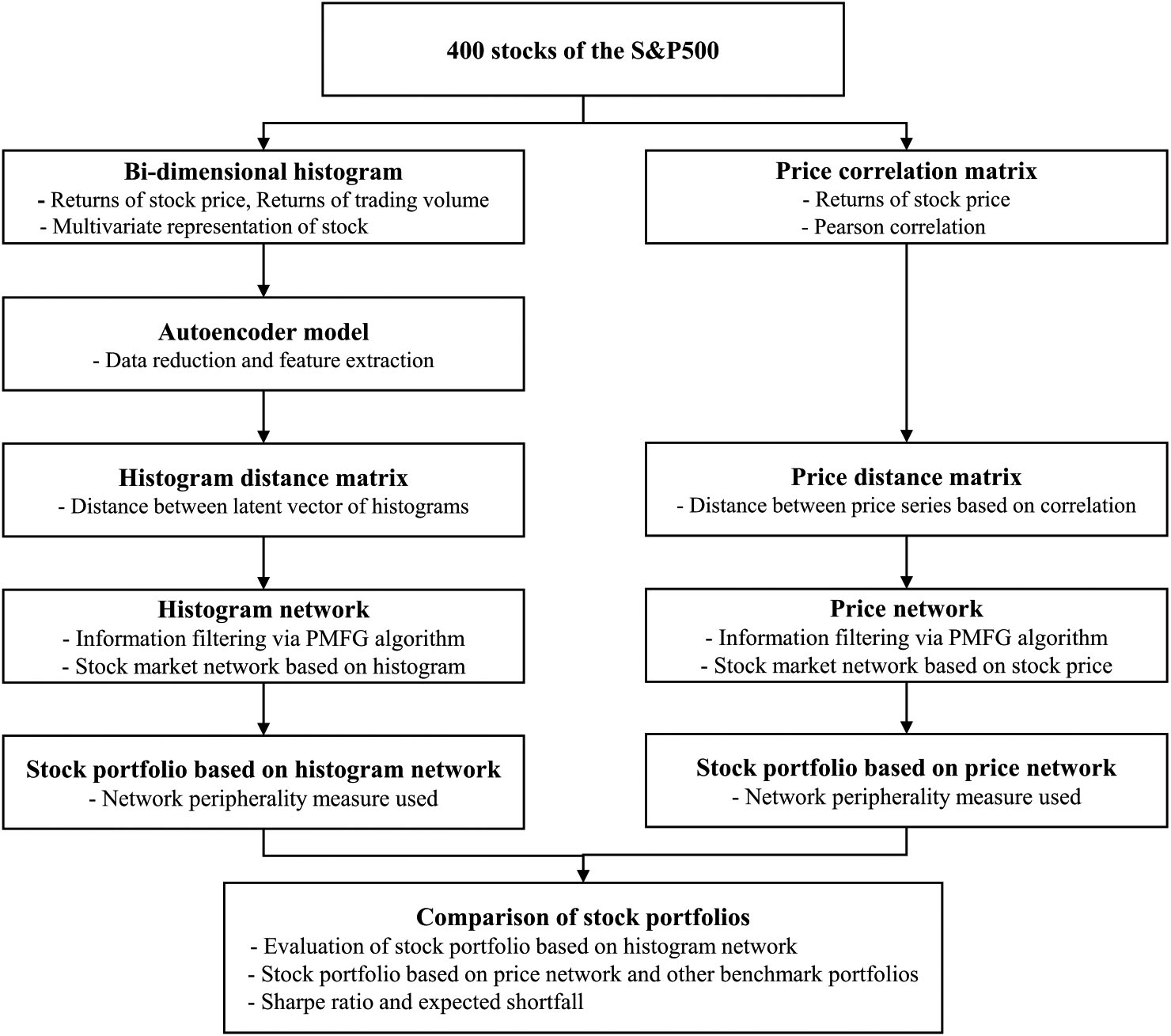

4. Experimental results

In this section, our experimental results are provided. The characteristics of bi-dimensional histogram for S&P500 stocks are studied. The network topologies are compared between the histogram network and the price network, and the investment usefulness of histogram network is examined.

4.1 Properties of bi-dimensional histogram

We analyze properties of the bi-dimensional histogram through $v_{H}$ , which approximates histogram dispersion. Figure 5a shows the distribution of $v_{H}$ based on the total of 128,400 bi-dimensional histograms for 400 stocks in each of 321 observation periods. The distribution of $v_{H}$ has the mean of 3.28, the standard deviation of 0.84, and is positively skewed. The result of Jaque-Bera goodness of fit test does not support that the distribution of $v_{H}$ is gaussian. Figure 5b shows that the distribution of $v_{H}$ is varied according to market conditions. The notations ‘before’, ‘during’, and ‘after’ correspond to 40 observation periods before, during, and after the financial crisis around 2008, respectively. The distribution of $v_{H}$ is left-biased and right skewed during the financial crisis period compared to the non-crisis period, before and after the crisis.

Table 4 presents the descriptive statistics of $v_{H}$ in each sub period and entire period. The mean and median of $v_{H}$ during the financial crisis are smaller than those of before and after crisis periods. Conversely, the standard deviation of $v_{H}$ during the crisis is relatively larger than those of before and after crisis periods. In Fig. 5b, the shifting of $v_{H}$ to the left during the crisis is related to the rigid market condition where stock price behavior loses diversity. The increment of average $v_{H}$ after financial crisis period can be interpreted as the stock market recovery where the behavior of stock prices becomes diverse.

Table 4
Descriptive statistics of $v_{H}$ for different periods

	Statistics
	Mean	Std	Max	Min	Median	Kurtosis	Skewness
Before crisis	3.21	0.84	6.88	1.15	3.12	0.24	0.50
During crisis	3.02	0.98	7.15	0.97	2.90	0.39	0.69
After crisis	3.39	0.89	8.23	1.24	3.36	0.14	0.39
Entire period	3.28	0.84	8.23	0.97	3.21	0.34	0.49

Figure 5.

Distribution of $v_{H}$ for entire period (a) and sub period:‘during’, ‘before’, ‘after’ (b).

For the analysis of $v_{H}$ in each industry, the stock is subdivided into 11 industry sectors based on GICS. Figure 6 shows the time series of the average value of $v_{H}$ for each industry sector. The evolution of $v_{H}$ is affected by market condition.

When focusing on the sub-prime mortgage crisis, the value of $v_{H}$ decreases for most of industries. The lower dispersion level of bi-dimensional histogram implies the less volatile stock market. During the sub-prime mortgage crisis, $v_{H}$ of COND, INDS and INFT decreased by 26%, 22% and 30% respectively in the short term. For FINC and REES, time series of $v_{H}$ shows ‘V’ pattern at the crisis, decreasing abruptly but rebounding rapidly. Stock prices of FINC and REES industries are quickly recovered after being directly affected by the crisis. CONS and UTIL are characterized by a low level of $v_{H}$ compared to other industries. The similar trend is also observed in the Chinese stock market turbulence in mid-2015.

Table 5 shows the correlation of $v_{H}$ for each pair of industry sector. Most of cases show a strong positive correlation. FINC and REES industries are negatively correlated with other industries, in general. Among 11 given correlation pairs for each industry sector, FINC and REES have 9 and 11 negative correlation pairs with other industry sectors. We also compute the correlation between an individual industry sector and S&P500 index. S&P500 index is marked as INDX. All industry sectors except for FINC and REES have a positive correlation with INDX, implying that the increment of S&P500 index leads to the high dispersion of bi-dimensional histogram for stocks in all sectors except for FINC and REES. FINC and REES industries have a $-$ 0.65 and $-$ 0.61 correlation with the S&P500 index, respectively. This means that the dispersion of the bi-dimensional histogram for FINC and REES decreases as the S&P500 index increases.

Figure 6.

Evolution of the series of $v_{H}$ for GICS sectors and S&P500 index.

Table 5

Correlation between $v_{H}$ of GICS sectors

	COMM	COND	CONS	ENRG	FINC	HLCA	INDS	INFT	MTRS	REES	UTIL
COND	0.63
CONS	0.82	0.57
ENRG	0.65	0.36	0.66
FINC	$-$ 0.19	0.15	$-$ 0.53	$-$ 0.33
HLCA	0.85	0.66	0.84	0.73	$-$ 0.24
INDS	0.69	0.74	0.49	0.44	0.17	0.78
INFT	0.69	0.79	0.71	0.54	$-$ 0.17	0.88	0.86
MTRS	0.69	0.73	0.65	0.75	0.02	0.86	0.76	0.81
REES	$-$ 0.38	0.04	$-$ 0.51	$-$ 0.54	0.71	$-$ 0.49	$-$ 0.14	$-$ 0.36	$-$ 0.29
UTIL	0.53	0.49	0.74	0.51	$-$ 0.26	0.67	0.34	0.52	0.59	$-$ 0.13
INDX	0.70	0.17	0.80	0.71	$-$ 0.65	0.57	0.18	0.33	0.36	$-$ 0.61	0.43

4.2 Dimensional reduction result of the bi-dimensional histogram

In this study, the Bi-dimensional histograms are 11 by 11 dimensions and have noise and missing values. Bi-dimensional histograms consist of 121 bins, and 50.7% of bins are empty. In addition, the bin whose frequency is less than 1% corresponds to 25% of the total. As such, the bi-dimensional histogram of stock has a large amount of noise. Therefore, we use an autoencoder to extract meaningful information from the bi-dimensional histogram. Figure 7 shows the bi-dimensional histogram of stocks and the reconstructed bi-dimensional histogram. The latent vector of the bi-dimensional histogram is 32 dimensions and has less noise and missing values compared to the bi-dimensional histogram. On average, 22% of the bins of the latent vector are noise. We calculate the distance matrix between latent vectors according to Eq. (6). And then, we apply the PMFG algorithm to the distance matrix to build a stock market network based on latent vector of bi-dimensional histogram. The experimental results for the properties of the bi-dimensional histogram network are continued in the next section.

Figure 7.

The original histogram and reconstructed histogram.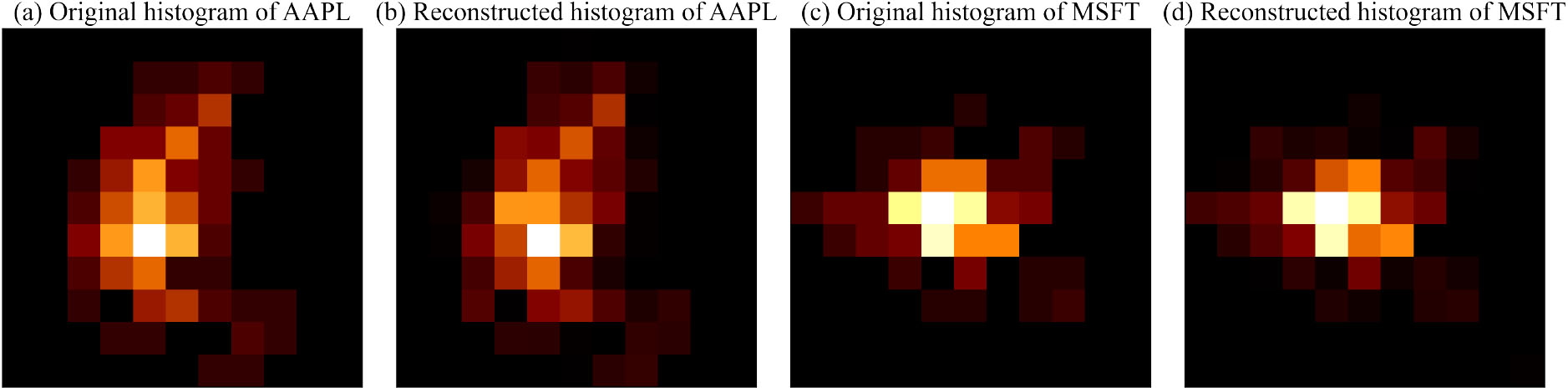

4.3 Properties of bi-dimensional histogram network

Latent vectors of bi-dimensional histograms for each stock are represented as nodes in the histogram network. Characteristics of each bi-dimensional histograms and their relationships are reflected in the topological structure of histogram network.

Figure 8.

Classification of nodes in the histogram network according to the level of 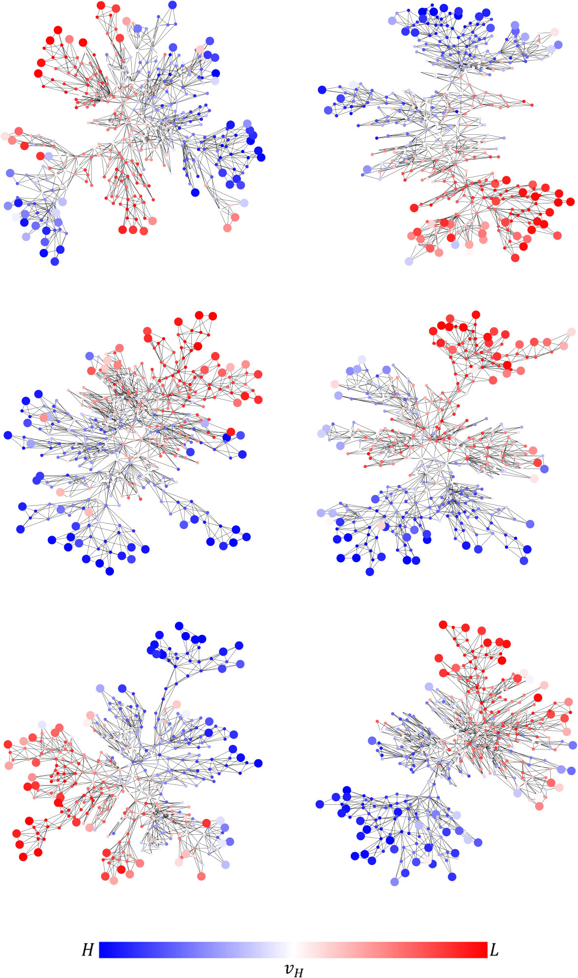$v_{H}$ .

Figure 8 shows 6 snapshots of the histogram network. The colors of node changing from blue to red correspond to the descending values of $v_{H}$ . In Fig. 8, we emphasize the nodes of top 60 peripherality values in Eq. (8) by varying their size in proportion to peripherality values to identify significant peripheral nodes. In the histogram network, nodes with larger $v_{H}$ colored in darker blue and nodes with smaller $v_{H}$ colored in darker red are located in the periphery of network.

Figure 9 shows the result of correlation analysis between $v_{H}$ and network topology measure of histogram network. The average shortest path length, peripherality, and betweenness, closeness, degree, and eigenvector centrality of nodes are used as network topology measures. The purpose of correlation analysis is to examine whether $v_{H}$ of the peripheral node is significantly larger or smaller than the central node. We analyze the correlation between the network topology measure and $\tilde{v}_{H}$ , which is defined as $\tilde{v}_{H}=\mid v_{H}-\overline{v}_{H}\mid$ where $\overline{v}_{H}$ is the average of $v_{H}$ . The analysis method is as follows. The top $N$ nodes and the bottom $N$ nodes are selected based on the network topology measure value in the network at time $t$ . Then, the correlation at time $t$ , $\rho_{N}(t)$ , between $\tilde{v}_{H}$ and the network topology measure value for a total of $2N$ nodes is calculated.

Figure 9.

Correlation between $\tilde{v}_{H}$ and network topology measure according to the number of nodes.

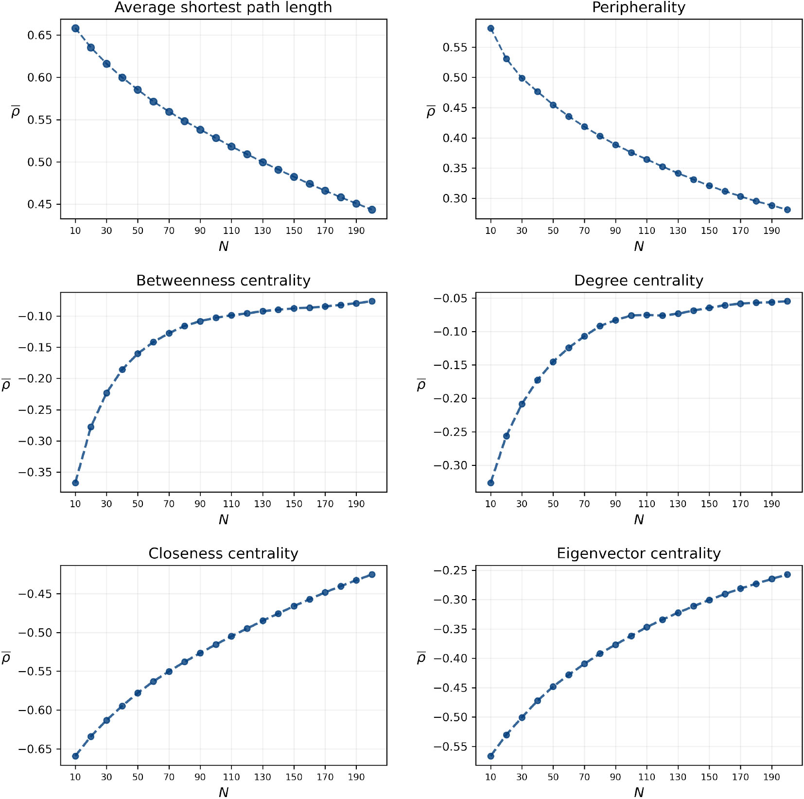
In Fig. 9 showing the variation of average of $\rho_{N}(t)$ against node size $N$ . In the histogram network, the positive correlation of $\tilde{v}_{H}$ with average shortest path length and peripherality, respectively, is observed. A positive correlation between $\tilde{v}_{H}$ and the average shortest path length implies that a node with the larger $\tilde{v}_{H}$ has the longer shortest path to other nodes in the network. As the nodes located in the periphery of the network tend to have the longer shortest path to other nodes, nodes with the larger $\tilde{v}_{H}$ (either larger $v_{H}$ or smaller $v_{H}$ ) are likely to be peripheral nodes of network as shown in Fig. 8. In the case of peripherality, the nodes with larger $\tilde{v}_{H}$ tend to have the higher periphery level. Although the correlation level decreases as the number of nodes, $N$ , increases for both average shortest path length and peripherality, the correlation values are still around 0.45 and 0.3 respectively, when including all nodes of network, showing a significant positive correlation.

Meanwhile, centrality measures including betweeness centrality (BC), degree centrality (DC), closeness centrality (CC), and eigenvector centrality (EC) are negatively correlated with $\tilde{v}_{H}$ unlike peripheral measures. Note that BC and DC measure the frequency of a node belonging to the shortest path in the network and the number of edges connected to a node, respectively. The nodes with larger $\tilde{v}_{H}$ tend to show lower level of BC and DC. As both BC and DC indicate the centrality level of a node, nodes with larger $\tilde{v}_{H}$ are observed in the periphery of network rather than the center. The correlations of $\tilde{v}_{H}$ with BC and degree DC decrease rapidly as $N$ increases. CC and EC, which become high value when the distance between nodes are short in general, show a clear negative correlation with $\tilde{v}_{H}$ , supporting that peripheral nodes have the larger $\tilde{v}_{H}$ than central nodes. The result of correlation analysis implies that the histogram network is suitable for reflecting the distributional characteristics of the stock, implying that the AE is effective in extracting the latent feature of the bi-dimensional histogram.

4.4 Comparison of histogram network with price network

Figure 10.

The top 20 and the bottom 20 nodes in each network according to peripherality.

This section compares the structural features of histogram network and price network. Figure 10 shows snapshots of histogram network and price network. The coloring nodes in the network indicate top 20 central nodes (circle shape) and top 20 peripheral nodes (rectangular shape), and each color of node refers to the corresponding industry sector. In price networks, the central nodes include FINC and INDS from 2006-01-03 to 2006-12-29 and INDS and INFT from 2008-09-16 to 2009-09-14, which corresponds to the financial crisis period. In the histogram network, the composition of central nodes and peripheral are more diverse than price network.

Table 6 presents the top 10 stock ranks based on the frequencies included in the top 10 central and peripheral nodes, respectively, over entire 321 observation periods. Stocks of the ENRG, INFT, and HLCA sectors are located in the periphery of histogram network mainly. Among them, AMD is most frequently located in the periphery of histogram network, with 53 times (17%). On the other hand, stocks of the UTIL, CONS, and ENRG industry sectors are located in the periphery of the price network.

NRG is most frequently located in the periphery of a price network, with 70 times (22%). In histogram networks, the frequency of a certain stock located in the periphery of network is much higher than that in the center of network. This implies that the characteristics of bi-dimensional histogram can be determined by the property of the peripheral nodes. The frequency that specific stocks are located in the center or periphery of network is much higher in price networks than histogram networks. Especially, the central nodes in price network have more tendency to belong to certain industry sectors. INDS and FINC sector are mainly located in the center of price networks, and ITW is located 92 times (29%) in the center.

Table 6

The frequency for nodes located in the center and periphery of network

Histogram network								Price network
Peripheral				Central				Peripheral				Central
Rank	Stock	Sector	Count	Rank	Stock	Sector	Count	Rank	Stock	Sector	Count	Rank	Stock	Sector	Count
1	AMD	INFT	53	1	TMO	HLCA	17	1	NRG	UTIL	70	1	ITW	INDS	92
2	URI	INDS	39	2	JCI	INDS	17	2	COG	ENRG	49	2	HON	INDS	86
3	JNJ	HLCA	37	3	IR	INDS	15	3	CAG	CONS	49	3	AMP	FINC	83
4	FCX	MTRS	36	4	AVY	MTRS	15	4	WMB	ENRG	48	4	TROW	FINC	78
5	XOM	ENRG	32	5	ANTM	HLCA	15	5	FE	UTIL	35	5	AMG	FINC	65
6	NVDA	INFT	20	6	DOV	INDS	14	6	TSN	CONS	34	6	IEX	INDS	58
7	WCG	HLCA	18	7	NSC	INDS	13	7	AES	UTIL	34	7	BEN	FINC	56
8	WYNN	COND	18	8	TXN	INFT	13	8	EXC	UTIL	33	8	BRK.B	FINC	52
9	PXD	ENRG	17	9	LEG	COND	13	9	CLX	CONS	32	9	BLK	FINC	49
10	XEC	ENRG	17	10	ETN	INDS	12	10	DLTR	COND	30	10	PFG	FINC	37

Table 7 presents descriptive statistics of histogram network and price network. The nodes having the most connectivity in histogram network and price network during the entire observation periods have 37 edges and 149 edges, respectively. The standard deviations of the degree of nodes are 3.52 for histogram network, and 5.87 for price network. This implies that a local cluster having the central hub node is more common in price network than histogram network.

For the diameter of the network, the longest path length between nodes, price network has the average diameter of 11.83 and bi-dimensional histogram network has the average diameter of 16.72 which is 41% larger than price network. Assortativity is an index for the network hub which is a node with many edges. If the assortativity of the network is positive, the hubs are clustered together. Conversely, the negative assortativity called a disassortative network means that nodes with few edges tend to be located around the hub. Both bi-dimensional histogram network and price network are disassortative networks, and price networks are more disassortative. According to the above results, the average shortest path length of price network is smaller than that of histogram network.

Table 7

Descriptive statistics of network topology measure

Measure	Statistics	Histogram network	Price network	Measure	Statistics	Histogram network	Price network
Degree	Mean	5.97	5.97	Diameter	Mean	16.72	11.83
	Std	3.52	5.87		Std	2.48	2.42
	Max	37.00	149.00		Max	26.00	20.00
	Min	3.00	3.00		Min	11.00	8.00
	Median	5.00	4.00		Median	16.00	11.00
	Kurtosis	5.23	91.78		Kurtosis	1.40	0.36
	Skewness	1.94	7.04		Skewness	0.93	0.87
	$p$ -value	0.00			$p$ -value	1.04E-83
Assortativity	Mean	$-$ 0.02	$-$ 0.10	Average shortest path length	Mean	6.60	4.81
	Std	0.03	0.02		Std	0.75	0.83
	Max	0.04	$-$ 0.05		Max	11.06	7.98
	Min	$-$ 0.10	$-$ 0.14		Min	5.06	3.52
	Median	$-$ 0.02	$-$ 0.10		Median	6.47	4.68
	Kurtosis	$-$ 0.15	0.10		Kurtosis	4.22	0.08
	Skewness	0.02	0.42		Skewness	1.37	0.84
	$p$ -value	8.73E-149			$p$ -value	1.59E-96

${}^{*}$ Note: $p$ -value means statistical significance for the results of two sample $t$ test.

Figure 11.

The proportion of stocks remaining in periphery (a) and center (b) of network after the time interval 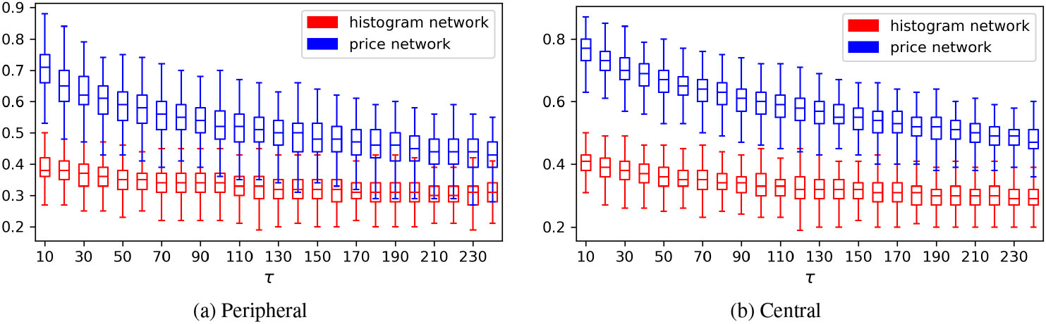$\tau$ .

Figure 11 shows the proportion of stocks remaining in the top 100 central nodes and the top 100 peripheral nodes after time interval $\tau$ . All peripheral nodes are selected using Eq. (8). In this way, we investigate how many nodes remain in the center and the periphery of the network as time goes. The proportion of remaining central nodes and peripheral nodes of price network gradually decreases from 80% to 60% as $\tau$ increases, while the proportion of remaining central nodes and peripheral nodes of histogram network decreases from 40% to 30%.

4.5 Application to stock portfolio

In this section, we construct portfolios using stocks corresponding to peripheral nodes of network. For the examination of portfolio performance, we use measures introduced in Section 3.3. Detailed results of the portfolio experiment are described in appendix Appendix B. Portfolio experiment results.

Tables B.1 shows the sharpe ratio for each strategy according to the number of stocks in the portfolio and the holding period. In histogram network, a portfolio of peripheral nodes shows the higher sharpe ratio than that of central nodes. This implies that a portfolio consisting of stocks located in the periphery of histogram network can be effective in that stocks have not only high sharp ratio but also few dependency on other stocks. Previous studies [44, 29, 31] also conclude that forming a portfolio using peripheral node stocks is the better strategy than using the central ones for the price network case.

Figure 12 presents the average sharpe ratio in terms of number of stocks, $N$ , for various portfolios. When comparing the sharpe ratio of histogram network portfolio with that of other benchmark portfolio, only the portfolio based on peripheral nodes of histogram network is superior to the market portfolio. For the network-based strategy, the portfolio of peripheral nodes has the higher sharpe ratio than that of central nodes. All the portfolios except for the mega-cap portfolio show the better performance than S&P 500 index.

Figure 12.

Sharpe ratio of various portfolios.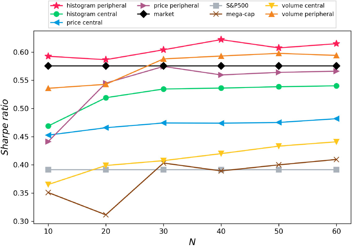

Figure 13.

Cumulative return of various portfolios.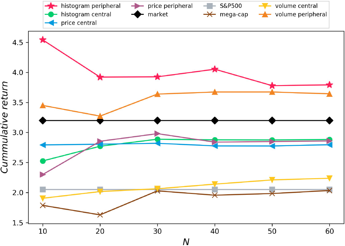

Table B.2 presents the result of cumulative return of portfolios for each strategy. For the cumulative return of portfolio based on histogram networks, cumulative return of portfolio using peripheral nodes is higher than that of portfolio using central nodes. On the other hand, for the cumulative return of portfolio based on price network, there is no significant difference between the portfolio using peripheral nodes and that using central nodes.

Figure 13 presents the average cumulative return of portfolios against the portfolio size, $N$ . When comparing the cumulative return of histogram network portfolios with other portfolios, the portfolio based on peripheral nodes of histogram network shows better performance than other portfolios. The portfolio based on peripheral nodes of histogram network gains 400% or more cumulative return compared to 320% cumulative return of market portfolio. The portfolios showing relatively poor cumulative return are the mega-cap portfolio and the S&P500 index portfolio.

Figure 14.

1% Expected shortfall of various portfolios.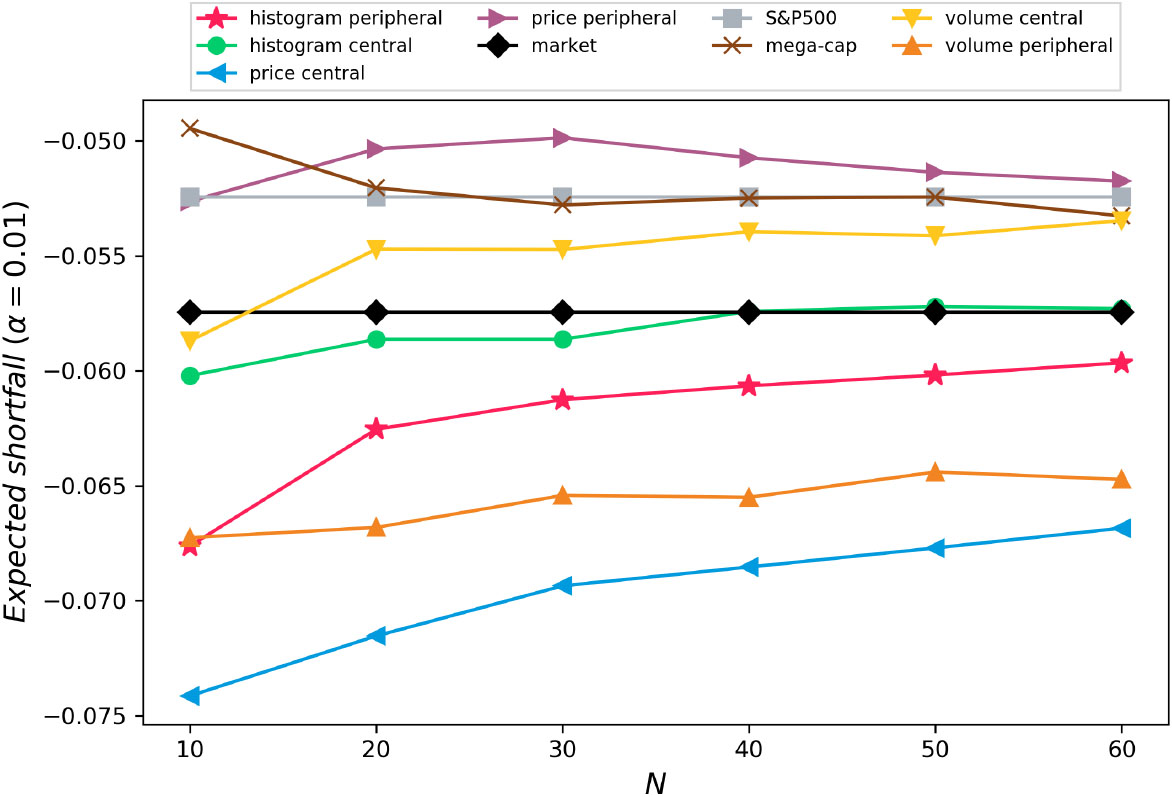

Finally, Table B.3 provides the results of 1% expected shortfall according to each portfolio strategy. When looking at the expected shortfall of portfolios in Fig. 14, the poorest portfolio in terms of risk is the portfolio of central nodes in price network. The portfolio of peripheral nodes in price network is the best strategy in terms of 1% expected shortfall. For histogram network portfolio, the portfolio of peripheral nodes in trading volume network is more risky than that of peripheral nodes in histogram network. Overall, the portfolio of peripheral nodes in histogram network is more risky in terms of 1% expected shortfall than the market portfolio and the portfolio of peripheral nodes in price network, but it has the best Sharpe ratio and cumulative return.

5. Conclusion

In this paper, we propose a deep learning related framework to analyze stock market with multidimensional data. We construct a bi-dimensional histogram using the returns of price and trading volume of stocks, and apply autoencoder to the bi-dimensional histogram to extract features, and build a stock market network using the PMFG algorithm. The proposed stock market network represents the latent space of bi-dimensional histogram of stock prices and trading volumes.

Our results show that stocks with larger or smaller histogram dispersion than usual are located in the periphery of histogram network, while stocks with moderate dispersion are located in the center of the network. The nodes of the histogram network are clustered according to the histogram dispersion, implying that the autoencoder is effective in extracting the latent feature of the bi-dimensional histogram.

The dispersion of the bi-dimensional histogram has properties related to market conditions, and tends to decrease when the diversity of stock movements decreases, for example the financial crisis. We examine time varying properties of bi-dimensional histogram of stocks categorized in 11 industry sectors based on GICS, and observe that the dispersion of histogram for each industry sector decreases during the crisis period. In detail, the dispersion of the histogram for stocks in the industry sensitive to economy condition rapidly decreases during the financial crisis period. The industry sector which is insensitive to the economy condition shows low level of dispersion compared to other industry sectors. The dispersion of histogram for stocks in FINC and REES industries are negatively correlated with the dispersion of other industries.

We observe clear structural differences between our suggested histogram network and conventional price network. Histogram network is relatively more assortative than price network. For the composition of stocks for peripheral and center nodes of network, histogram network is distinct from price network. In the price network, stocks of the industrial and financial industries are located in the center, and stocks of utilities, energy and consumer staples industries are located in the periphery. On the other hand, for histogram network stocks of health care and industrial industries are located in the center, and stocks of information technology and energy industries are located in the periphery.

We found that the usage of stock trading volume on top of stock price information can leads to the improvement of stock portfolio performance. The portfolio using the peripheral nodes of histogram network shows a higher Sharpe ratio than the portfolio based on central nodes of histogram network, the market portfolio and other benchmarks including the portfolio using price network. Overall, investment portfolio based on peripheral nodes of histogram network using stock prices and trading volumes outperforms other benchmarks.

As future work, we can extend the bi-dimensional histogram network into the higher dimensional histogram network using more information such as accounting variables in addition to stock price and stock trading volume. We expect that the inclusion of more information on stocks to our framework can improve the performance of stock portfolio based on multi-dimensional histogram network.

Footnotes

Acknowledgments

This work was supported by the National Research Foundation of Korea (NRF) grant funded by the Ministry of Science and ICT (No. 2018R1C1B5043835).

Credit authorship contribution statement

Sungyoun Choi designed the bi-dimensional histogram and developed the auto-encoder model. Choi constructed the bi-dimensional histogram network using histogram distance matrix and the stock portfolio based on the histogram network. Dongkyu Gwak computed the price correlation matrix and price distance matrix. Gwak built the price network and constructed the stock portfolio based on the price network. Jae Wook Song performed the comparison analysis between the stock portfolios. Woojin Chang advised the overall research and experiment procedures.

Appendix

Appendix A. Selected stocks for experiment

We select 400 stocks that have been fully listed in S&P500 from January 3, 2006 to September 30, 2019. The list of stocks selected for the experiment is summarized in Tables A.1 and A.2.

Table A.1

Stock list

GICS sector	Symbol	Security	GICS sector	Symbol	Security	GICS sector	Symbol	Security
Communication	ATVI	Activision Blizzard	Consumer	MO	Altria Group Inc	Financials	COF	Capital One Financial
Services	GOOGL	Alphabet Inc.	Staples	ADM	Archer-Daniels-Midland Co		SCHW	Charles Schwab Corporation
	T	AT&T Inc.		BF.B	Brown-Forman Corp.		CB	Chubb Limited
	CBS	CBS		CPB	Campbell Soup		CINF	Cincinnati Financial
	CTL	CenturyLink Inc		CHD	Church & Dwight		C	Citigroup Inc.
	CMCSA	Comcast Corp.		KO	Coca-Cola Company		CME	CME Group Inc.
	DISCA	Discovery, Inc.		CL	Colgate-Palmolive		CMA	Comerica Inc.
	DISH	Dish Network		CAG	Conagra Brands		ETFC	E*Trade
	EA	Electronic Arts		STZ	Constellation Brands		RE	Everest Re Group Ltd.
	IPG	Interpublic Group		COST	Costco Wholesale Corp.		FITB	Fifth Third Bancorp
	OMC	Omnicom Group		EL	Este Lauder Companies		BEN	Franklin Resources
	DIS	The Walt Disney Company		GIS	General Mills		GL	Globe Life Inc.
	VZ	Verizon Communications		HRL	Hormel Foods Corp.		GS	Goldman Sachs Group
	VIAB	Viacom		SJM	JM Smucker		HIG	Hartford Financial Svc.Gp.
Consumer	AAP	Advance Auto Parts		K	Kellogg Co.		HBAN	Huntington Bancshares
Discretionary	AMZN	Amazon.com Inc.		KMB	Kimberly-Clark		ICE	Intercontinental Exchange
	AZO	AutoZone Inc		KR	Kroger Co.		JPM	JPMorgan Chase & Co.
	BBY	Best Buy Co. Inc.		MKC	McCormick & Co.		KEY	KeyCorp
	BWA	BorgWarner		TAP	Molson Coors Brewing Company		LNC	Lincoln National
	KMX	Carmax Inc		MDLZ	Mondelez International		L	Loews Corp.
	CCL	Carnival Corp.		MNST	Monster Beverage		MTB	M&T Bank Corp.
	DHI	D. R. Horton		PEP	PepsiCo Inc.		MMC	Marsh & McLennan
	DRI	Darden Restaurants		PG	Procter & Gamble		MET	MetLife Inc.
	DLTR	Dollar Tree		SYY	Sysco Corp.		MCO	Moody’s Corp
	EBAY	eBay Inc.		CLX	The Clorox Company		MS	Morgan Stanley
	EXPE	Expedia Group		HSY	The Hershey Company		NDAQ	Nasdaq, Inc.
	F	Ford Motor Company		TSN	Tyson Foods		NTRS	Northern Trust Corp.
	GPS	Gap Inc.		WBA	Walgreens Boots Alliance		PBCT	People’s United Financial
	GRMN	Garmin Ltd.		WMT	Walmart		PNC	PNC Financial Services
	GPC	Genuine Parts	Energy	APA	Apache Corporation		PFG	Principal Financial Group
	HRB	H&R Block		BHGE	BAKER HUGHES		PGR	Progressive Corp.
	HOG	Harley-Davidson		COG	Cabot Oil & Gas		PRU	Prudential Financial
	HAS	Hasbro Inc.		CVX	Chevron Corp.		RJF	Raymond James Financial Inc.
	HD	Home Depot		XEC	Cimarex Energy		RF	Regions Financial Corp.
	KSS	Kohl’s Corp.		COP	ConocoPhillips		SPGI	S&P Global, Inc.
	LB	L Brands Inc.		DVN	Devon Energy		STT	State Street Corp.
	LVS	Las Vegas Sands		EOG	EOG Resources		STI	SunTrust Banks
	LEG	Leggett & Platt		XOM	Exxon Mobil Corp.		SIVB	SVB Financial
	LEN	Lennar Corp.		HAL	Halliburton Co.		TROW	T. Rowe Price Group
	LOW	Lowe’s Cos.		HES	Hess Corporation		BK	The Bank of New York Mellon
	M	Macy’s, Inc.		HFC	HollyFrontier Corp		TRV	The Travelers Companies Inc.
	MAR	Marriott Int’l.		HP	HP		USB	U.S. Bancorp
	MCD	McDonald’s Corp.		MRO	Marathon Oil Corp.		UNM	Unum Group
	MGM	MGM Resorts International		NOV	National Oilwell Varco Inc.		WFC	Wells Fargo
	MHK	Mohawk Industries		NBL	Noble Energy Inc		WLTW	Willis Towers Watson
	NWL	Newell Brands		OXY	Occidental Petroleum		ZION	Zions Bancorp
	NKE	Nike		OKE	ONEOK	Health	ABT	Abbott Laboratories
	JWN	Nordstrom		PXD	Pioneer Natural Resources	Care	A	Agilent Technologies Inc
	NVR	NVR Inc		SLB	Schlumberger Ltd.		AGN	Allergan
	ORLY	O’Reilly Automotive		VLO	Valero Energy		ABC	AmerisourceBergen Corp
	PHM	PulteGroup		WMB	Williams Cos.		AMGN	Amgen Inc.
	RL	Ralph Lauren Corporation	Financials	AFL	AFLAC Inc		ANTM	Anthem
	ROST	Ross Stores		ALL	Allstate Corp		BAX	Baxter International Inc.
	RCL	Royal Caribbean Cruises Ltd		AXP	American Express Co		BDX	Becton Dickinson
	SBUX	Starbucks Corp.		AIG	American International Group		BIIB	Biogen Inc.
	TPR	Tapestry, Inc.		AMP	Ameriprise Financial		BSX	Boston Scientific
	TGT	Target Corp.		AMG	AMGEN		BMY	Bristol-Myers Squibb
	TIF	Tiffany & Co.		AON	Aon plc		CAH	Cardinal Health Inc.
	TJX	TJX Companies Inc.		AJG	Arthur J. Gallagher & Co.		CERN	Cerner
	TSCO	Tractor Supply Company		AIZ	Assurant		CI	CIGNA Corp.
	VFC	V.F. Corp.		BAC	Bank of America Corp		CVS	CVS Health
	WHR	Whirlpool Corp.		BBT	BB&T		DHR	Danaher Corp.
	WYNN	Wynn Resorts Ltd		BRK.B	Berkshire Hathaway		DVA	DaVita Inc.
	YUM	Yum! Brands Inc		BLK	BlackRock		XRAY	Dentsply Sirona

Table A.2

Stock list (continued)

GICS sector	Symbol	Security	GICS sector	Symbol	Security	GICS sector	Symbol	Security
Health	EW	Edwards Lifesciences	Industrials	RSG	Republic Services Inc	Materials	FCX	Freeport-McMoRan Inc.
Care	GILD	Gilead Sciences		RHI	Robert Half International		IP	International Paper
	HSIC	Henry Schein		ROK	Rockwell Automation Inc.		IFF	Intl Flavors & Fragrances
	HOLX	Hologic		ROP	Roper Technologies		LIN	Linde plc
	HUM	Humana Inc.		SNA	Snap-on		MLM	Martin Marietta Materials
	IDXX	IDEXX Laboratories		LUV	Southwest Airlines		NEM	Newmont Corporation
	ISRG	Intuitive Surgical Inc.		SWK	Stanley Black & Decker		NUE	Nucor Corp.
	JNJ	Johnson & Johnson		TXT	Textron Inc.		PKG	Packaging Corporation of America
	LH	Laboratory Corp. of America Holding		UNP	Union Pacific Corp		PPG	PPG Industries
	LLY	Lilly (Eli) & Co.		UPS	United Parcel Service		SEE	Sealed Air
	MCK	McKesson Corp.		URI	United Rentals, Inc.		SHW	Sherwin-Williams
	MDT	Medtronic plc		UTX	UNITED TECHNOLOGIES		MOS	The Mosaic Company
	MRK	Merck & Co.		WM	Waste Management Inc.		VMC	Vulcan Materials
	MTD	Mettler Toledo	Information	ACN	Accenture plc	Real	ARE	Alexandria Real Estate Equities
	MYL	Mylan N.V.	Technology	ADBE	Adobe Inc.	Estate	AMT	American Tower Corp.
	PKI	PerkinElmer		AMD	Advanced Micro Devices Inc		AIV	Apartment Investment & Management
	PFE	Pfizer Inc.		AKAM	Akamai Technologies Inc		AVB	AvalonBay Communities
	DGX	Quest Diagnostics		ADS	Alliance Data Systems		BXP	Boston Properties
	RMD	ResMed		APH	Amphenol Corp		CBRE	CBRE Group
	SYK	Stryker Corp.		ADI	Analog Devices, Inc.		CCI	Crown Castle International Corp.
	TFX	Teleflex		AAPL	Apple Inc.		DRE	Duke Realty Corp
	COO	The Cooper Companies		AMAT	Applied Materials Inc.		EQR	Equity Residential
	TMO	Thermo Fisher Scientific		ADSK	Autodesk Inc.		ESS	Essex Property Trust, Inc.
	UNH	United Health Group Inc.		ADP	Automatic Data Processing		FRT	Federal Realty Investment Trust
	UHS	Universal Health Services, Inc.		CDNS	Cadence Design Systems		HCP	HCP
	VAR	Varian Medical Systems		CSCO	Cisco Systems		HST	Host Hotels & Resorts
	VRTX	node Pharmaceuticals Inc		CTXS	Citrix Systems		IRM	Iron Mountain Incorporated
	WAT	Waters Corporation		CTSH	Cognizant Technology Solutions		KIM	Kimco Realty
	WCG	WELLCARE HEALTH PLANS		GLW	Corning Inc.		MAC	MACERICH
	ZBH	Zimmer Biomet Holdings		DXC	DXC Technology		PLD	Prologis
	CELG	CELGENE		FFIV	F5 Networks		PSA	Public Storage
Industrials	MMM	3M Company		FIS	Fidelity National Information Services		O	Realty Income Corporation
	AME	AMETEK Inc.		FISV	Fiserv Inc		REG	Regency Centers Corporation
	ARNC	ARCONIC		FLIR	FLIR Systems		SBAC	SBA Communications
	BA	Boeing Company		GPN	Global Payments Inc.		SPG	Simon Property Group Inc
	CHRW	C. H. Robinson Worldwide		HPQ	HP Inc.		SLG	SL Green Realty
	CAT	Caterpillar Inc.		INTC	Intel Corp.		UDR	UDR, Inc.
	CTAS	Cintas Corporation		IBM	International Business Machines		VTR	Ventas Inc
	CPRT	Copart Inc		INTU	Intuit Inc.		VNO	Vornado Realty Trust
	CSX	CSX Corp.		JKHY	Jack Henry & Associates		WELL	Welltower Inc.
	CMI	Cummins Inc.		JNPR	Juniper Networks		WY	Weyerhaeuser
	DE	Deere & Co.		KLAC	KLA Corporation	Utilities	AES	AES Corp
	DOV	Dover Corporation		LRCX	Lam Research		LNT	Alliant Energy Corp
	ETN	Eaton Corporation		MXIM	Maxim Integrated Products Inc		AEE	Ameren Corp
	EMR	Emerson Electric Company		MCHP	Microchip Technology		AEP	American Electric Power
	EFX	Equifax Inc.		MU	Micron Technology		ATO	Atmos Energy
	EXPD	Expeditors		MSFT	Microsoft Corp.		CNP	CenterPoint Energy
	FAST	Fastenal Co		MSI	Motorola Solutions Inc.		CMS	CMS Energy
	FDX	FedEx Corporation		NTAP	NetApp		ED	Consolidated Edison
	FLS	Flowserve Corporation		NVDA	Nvidia Corporation		D	Dominion Energy
	GD	General Dynamics		ORCL	Oracle Corp.		DTE	DTE Energy Co.
	GE	General Electric		PAYX	Paychex Inc.		DUK	Duke Energy
	GWW	Grainger (W.W.) Inc.		QCOM	QUALCOMM Inc.		EIX	Edison Int’l
	HON	Honeywell Int’l Inc.		CRM	Salesforce.com		ETR	Entergy Corp.
	IEX	IDEX Corporation		STX	Seagate Technology		EVRG	Evergy
	ITW	Illinois Tool Works		SYMC	SYMANTEC		ES	Eversource Energy
	IR	Ingersoll Rand		SNPS	Synopsys Inc.		EXC	Exelon Corp.
	JBHT	J. B. Hunt Transport Services		TXN	Texas Instruments		FE	FirstEnergy Corp
	JEC	JACOBS ENGR		VRSN	Verisign Inc.		NEE	NextEra Energy
	JCI	Johnson Controls International		WDC	Western Digital		NI	NiSource Inc.
	KSU	Kansas City Southern		XRX	Xerox		NRG	NRG Energy
	LHX	L3Harris Technologies		XLNX	Xilinx		PNW	Pinnacle West Capital
	LMT	Lockheed Martin Corp.	Materials	APD	Air Products & Chemicals Inc		PPL	PPL Corp.
	MAS	Masco Corp.		ALB	Albemarle Corp		PEG	Public Serv. Enterprise Inc.
	NSC	Norfolk Southern Corp.		AVY	Avery Dennison Corp		SRE	Sempra Energy
	NOC	Northrop Grumman		BLL	Ball Corp		SO	Southern Company
	PCAR	PACCAR Inc.		CE	Celanese		WEC	WEC Energy Group
	PH	Parker-Hannifin		EMN	Eastman Chemical		XEL	Xcel Energy Inc
	PNR	Pentair plc		ECL	Ecolab Inc.
	RTN	Raytheon Company		FMC	FMC Corporation

Appendix B. Portfolio experiment results

Table B.1

Sharpe Ratio of portfolios

		10	20	30	40	50	60	70	80	90	100	110	120	130	140	150	160	170	180	190	200	210	220	230	240	Mean
		Holding period
Hist peripheral	$N=$ 10	0.63	0.52	0.54	0.63	0.73	0.58	0.75	0.58	0.66	0.62	0.85	0.45	0.73	0.57	0.49	0.51	0.53	0.58	0.43	0.65	0.70	0.55	0.45	0.49	0.59
	$N=$ 20	0.63	0.60	0.52	0.68	0.66	0.66	0.67	0.61	0.62	0.55	0.74	0.48	0.63	0.54	0.55	0.57	0.53	0.61	0.47	0.53	0.68	0.56	0.46	0.53	0.59
	$N=$ 30	0.62	0.59	0.58	0.68	0.65	0.66	0.71	0.66	0.62	0.62	0.73	0.53	0.62	0.58	0.50	0.62	0.50	0.63	0.54	0.61	0.65	0.57	0.48	0.55	0.60
	$N=$ 40	0.66	0.63	0.60	0.73	0.64	0.67	0.71	0.70	0.63	0.61	0.72	0.56	0.60	0.61	0.54	0.61	0.53	0.63	0.56	0.59	0.67	0.62	0.53	0.59	0.62
	$N=$ 50	0.57	0.58	0.56	0.67	0.61	0.66	0.67	0.65	0.59	0.62	0.69	0.54	0.63	0.62	0.53	0.58	0.53	0.64	0.58	0.61	0.69	0.66	0.52	0.58	0.61
	$N=$ 60	0.59	0.60	0.57	0.67	0.65	0.65	0.69	0.65	0.60	0.62	0.69	0.56	0.60	0.64	0.56	0.58	0.55	0.64	0.57	0.62	0.69	0.65	0.54	0.58	0.61
Hist central	$N=$ 10	0.50	0.44	0.48	0.34	0.36	0.49	0.45	0.36	0.53	0.48	0.46	0.57	0.51	0.46	0.45	0.39	0.50	0.57	0.62	0.52	0.47	0.35	0.49	0.47	0.47
	$N=$ 20	0.50	0.51	0.49	0.51	0.46	0.43	0.53	0.42	0.57	0.57	0.53	0.56	0.60	0.50	0.50	0.47	0.52	0.56	0.57	0.61	0.54	0.52	0.46	0.54	0.52
	$N=$ 30	0.56	0.55	0.56	0.54	0.46	0.51	0.56	0.48	0.52	0.56	0.49	0.57	0.54	0.54	0.45	0.56	0.54	0.51	0.57	0.61	0.55	0.55	0.44	0.60	0.53
	$N=$ 40	0.54	0.54	0.57	0.51	0.45	0.52	0.55	0.43	0.55	0.53	0.50	0.57	0.56	0.56	0.50	0.50	0.56	0.52	0.57	0.58	0.56	0.58	0.48	0.62	0.54
	$N=$ 50	0.53	0.53	0.56	0.50	0.47	0.50	0.55	0.44	0.55	0.52	0.53	0.56	0.54	0.57	0.53	0.52	0.61	0.50	0.56	0.56	0.56	0.60	0.52	0.61	0.54
	$N=$ 60	0.54	0.54	0.55	0.51	0.46	0.51	0.53	0.45	0.55	0.55	0.52	0.56	0.56	0.57	0.53	0.55	0.60	0.49	0.55	0.57	0.56	0.59	0.51	0.60	0.54
Pearson peripheral	$N=$ 10	0.51	0.40	0.36	0.51	0.49	0.39	0.53	0.45	0.35	0.63	0.23	0.41	0.23	0.49	0.47	0.42	0.65	0.46	0.37	0.50	0.42	0.39	0.53	0.39	0.44
	$N=$ 20	0.68	0.61	0.53	0.66	0.64	0.45	0.57	0.60	0.49	0.67	0.49	0.44	0.43	0.51	0.61	0.55	0.64	0.51	0.55	0.59	0.43	0.48	0.53	0.42	0.54
	$N=$ 30	0.65	0.68	0.56	0.74	0.58	0.55	0.63	0.60	0.58	0.62	0.55	0.52	0.50	0.53	0.61	0.55	0.66	0.56	0.59	0.57	0.49	0.56	0.47	0.43	0.57
	$N=$ 40	0.62	0.59	0.53	0.62	0.57	0.46	0.62	0.55	0.50	0.56	0.56	0.51	0.60	0.55	0.64	0.55	0.64	0.52	0.63	0.56	0.53	0.59	0.47	0.45	0.56
	$N=$ 50	0.62	0.61	0.56	0.63	0.53	0.49	0.60	0.55	0.50	0.56	0.55	0.52	0.61	0.57	0.59	0.59	0.61	0.54	0.63	0.59	0.53	0.59	0.50	0.48	0.56
	$N=$ 60	0.60	0.59	0.55	0.59	0.58	0.52	0.57	0.56	0.53	0.58	0.60	0.53	0.58	0.55	0.62	0.58	0.57	0.58	0.62	0.58	0.51	0.59	0.51	0.48	0.57
Pearson cental	$N=$ 10	0.50	0.54	0.56	0.48	0.53	0.43	0.50	0.42	0.46	0.41	0.43	0.39	0.35	0.41	0.54	0.52	0.39	0.35	0.34	0.40	0.45	0.51	0.49	0.47	0.45
	$N=$ 20	0.52	0.51	0.53	0.50	0.50	0.42	0.53	0.45	0.47	0.43	0.46	0.42	0.44	0.42	0.51	0.51	0.41	0.39	0.40	0.46	0.45	0.49	0.45	0.51	0.47
	$N=$ 30	0.55	0.53	0.52	0.50	0.52	0.44	0.52	0.48	0.49	0.47	0.42	0.45	0.44	0.42	0.51	0.52	0.45	0.43	0.40	0.46	0.47	0.43	0.49	0.49	0.47
	$N=$ 40	0.53	0.50	0.52	0.46	0.51	0.47	0.50	0.48	0.48	0.47	0.41	0.46	0.44	0.42	0.50	0.51	0.47	0.41	0.42	0.46	0.50	0.42	0.52	0.50	0.47
	$N=$ 50	0.54	0.51	0.51	0.47	0.52	0.47	0.51	0.47	0.47	0.48	0.42	0.47	0.46	0.44	0.47	0.51	0.47	0.43	0.43	0.47	0.49	0.39	0.50	0.50	0.48
	$N=$ 60	0.51	0.50	0.50	0.48	0.52	0.48	0.50	0.49	0.48	0.50	0.42	0.50	0.47	0.47	0.47	0.51	0.47	0.45	0.44	0.48	0.50	0.42	0.50	0.51	0.48
Volume peripheral	$N=$ 10	0.71	0.55	0.44	0.44	0.51	0.44	0.53	0.50	0.71	0.52	0.53	0.46	0.63	0.50	0.59	0.43	0.70	0.69	0.62	0.50	0.55	0.41	0.50	0.39	0.54
	$N=$ 20	0.66	0.49	0.48	0.46	0.56	0.49	0.53	0.41	0.60	0.58	0.49	0.58	0.66	0.54	0.56	0.38	0.65	0.56	0.65	0.52	0.58	0.50	0.54	0.52	0.54
	$N=$ 30	0.64	0.53	0.52	0.55	0.60	0.56	0.51	0.48	0.69	0.61	0.56	0.61	0.68	0.54	0.65	0.47	0.66	0.67	0.62	0.62	0.60	0.57	0.65	0.53	0.59
	$N=$ 40	0.61	0.53	0.54	0.54	0.56	0.58	0.51	0.51	0.68	0.60	0.56	0.63	0.64	0.55	0.65	0.51	0.67	0.69	0.65	0.62	0.60	0.55	0.66	0.58	0.59
	$N=$ 50	0.61	0.58	0.54	0.55	0.55	0.57	0.55	0.56	0.66	0.63	0.53	0.67	0.60	0.56	0.59	0.55	0.67	0.67	0.66	0.65	0.59	0.53	0.67	0.60	0.60
	$N=$ 60	0.57	0.58	0.51	0.55	0.56	0.58	0.54	0.57	0.64	0.60	0.55	0.67	0.59	0.53	0.57	0.56	0.69	0.68	0.65	0.65	0.57	0.56	0.68	0.64	0.59
Volume central	$N=$ 10	0.35	0.41	0.44	0.34	0.45	0.36	0.54	0.37	0.41	0.43	0.35	0.27	0.30	0.48	0.36	0.37	0.33	0.35	0.30	0.35	0.36	0.26	0.39	0.21	0.37
	$N=$ 20	0.46	0.52	0.41	0.43	0.48	0.40	0.49	0.46	0.38	0.46	0.36	0.34	0.44	0.47	0.38	0.40	0.28	0.32	0.32	0.40	0.37	0.36	0.38	0.28	0.40
	$N=$ 30	0.46	0.46	0.37	0.41	0.48	0.35	0.52	0.47	0.40	0.44	0.35	0.32	0.49	0.47	0.42	0.44	0.31	0.34	0.44	0.44	0.39	0.35	0.36	0.31	0.41
	$N=$ 40	0.53	0.46	0.38	0.44	0.50	0.36	0.56	0.46	0.44	0.46	0.33	0.34	0.43	0.46	0.44	0.46	0.32	0.36	0.46	0.41	0.41	0.36	0.36	0.33	0.42
	$N=$ 50	0.54	0.50	0.42	0.44	0.47	0.40	0.54	0.46	0.47	0.45	0.33	0.40	0.44	0.46	0.47	0.49	0.33	0.41	0.46	0.41	0.43	0.38	0.35	0.34	0.43
	$N=$ 60	0.52	0.49	0.44	0.45	0.48	0.39	0.54	0.46	0.48	0.48	0.34	0.41	0.44	0.47	0.50	0.47	0.35	0.42	0.46	0.44	0.43	0.39	0.38	0.35	0.44
Market cap – mega	$N=$ 10	0.34	0.33	0.35	0.34	0.35	0.34	0.33	0.36	0.38	0.40	0.31	0.34	0.36	0.32	0.40	0.37	0.34	0.34	0.36	0.33	0.34	0.35	0.39	0.37	0.35
	$N=$ 20	0.30	0.31	0.27	0.31	0.30	0.32	0.32	0.33	0.30	0.31	0.25	0.32	0.32	0.32	0.36	0.31	0.34	0.28	0.32	0.35	0.39	0.27	0.33	0.26	0.31
	$N=$ 30	0.44	0.43	0.42	0.40	0.40	0.41	0.44	0.41	0.40	0.39	0.39	0.39	0.41	0.42	0.41	0.42	0.38	0.34	0.41	0.41	0.41	0.39	0.37	0.36	0.40
	$N=$ 40	0.38	0.38	0.36	0.40	0.40	0.37	0.41	0.40	0.38	0.40	0.38	0.37	0.37	0.40	0.42	0.41	0.37	0.33	0.36	0.42	0.42	0.42	0.40	0.38	0.39
	$N=$ 50	0.41	0.41	0.40	0.41	0.40	0.39	0.40	0.40	0.42	0.40	0.40	0.38	0.38	0.40	0.42	0.40	0.39	0.36	0.37	0.43	0.42	0.43	0.40	0.38	0.40
	$N=$ 60	0.41	0.40	0.41	0.42	0.40	0.40	0.43	0.43	0.42	0.42	0.42	0.37	0.38	0.42	0.43	0.44	0.40	0.37	0.38	0.43	0.43	0.43	0.40	0.40	0.41
Market portfolio	$N=$ 400	0.58	0.58	0.57	0.58	0.58	0.57	0.58	0.58	0.58	0.58	0.57	0.57	0.57	0.57	0.58	0.58	0.57	0.57	0.56	0.58	0.58	0.57	0.57	0.57	0.58
S&P500 index		0.40	0.40	0.39	0.40	0.40	0.39	0.40	0.40	0.40	0.40	0.39	0.38	0.38	0.38	0.40	0.40	0.38	0.38	0.37	0.40	0.40	0.38	0.37	0.38	0.39

Table B.2

Cumulative return of portfolios

		10	20	30	40	50	60	70	80	90	100	110	120	130	140	150	160	170	180	190	200	210	220	230	240	Mean
		Holding period
Hist peripheral	$N=$ 10	5.22	3.65	4.07	5.00	8.37	4.88	7.16	4.33	5.77	4.42	8.15	2.70	5.94	3.74	2.81	3.07	3.15	3.90	2.92	4.86	6.09	2.99	2.26	3.53	4.54
	$N=$ 20	4.53	4.08	3.36	5.17	5.68	5.22	4.73	4.35	4.41	3.41	5.51	2.84	4.27	3.19	3.04	3.23	3.00	4.14	2.84	3.16	4.71	3.08	2.60	3.59	3.92
	$N=$ 30	4.21	3.92	3.98	4.95	5.20	4.98	4.95	4.69	4.43	4.03	4.88	3.14	4.05	3.36	2.59	3.77	2.60	4.40	3.37	3.63	4.07	2.93	2.60	3.52	3.93
	$N=$ 40	4.68	4.34	4.09	5.61	4.80	4.98	4.91	5.09	4.42	3.82	4.73	3.36	3.69	3.71	2.91	3.70	2.93	4.24	3.36	3.42	4.32	3.21	3.04	3.94	4.05
	$N=$ 50	3.59	3.76	3.59	4.75	4.07	4.67	4.37	4.38	3.93	3.74	4.34	3.15	3.98	3.73	2.77	3.34	2.87	4.28	3.42	3.54	4.35	3.48	2.86	3.74	3.78
	$N=$ 60	3.68	3.86	3.59	4.67	4.52	4.36	4.58	4.30	3.89	3.72	4.38	3.25	3.64	3.90	3.03	3.29	2.96	4.13	3.36	3.48	4.35	3.39	2.94	3.74	3.79
Hist central	$N=$ 10	2.84	2.40	2.63	1.81	1.97	2.71	2.39	1.89	2.95	2.59	2.56	3.01	3.09	2.50	2.40	2.05	2.38	3.03	3.73	2.76	2.40	1.60	2.48	2.47	2.53
	$N=$ 20	2.75	2.78	2.64	2.76	2.51	2.24	2.86	2.18	3.10	3.19	2.97	2.95	3.51	2.53	2.54	2.53	2.43	2.79	3.22	3.42	2.76	2.60	2.20	3.06	2.77
	$N=$ 30	3.18	3.10	3.19	2.93	2.55	2.80	3.09	2.50	2.83	3.13	2.61	3.10	2.93	2.88	2.26	3.18	2.65	2.71	3.09	3.35	2.89	2.81	2.11	3.46	2.89
	$N=$ 40	3.00	3.01	3.19	2.70	2.40	2.81	3.02	2.25	2.97	2.86	2.72	3.11	3.03	3.04	2.60	2.70	2.81	2.74	3.06	3.12	2.94	2.98	2.37	3.63	2.88
	$N=$ 50	2.95	2.92	3.13	2.69	2.50	2.70	3.00	2.24	2.89	2.77	2.98	3.03	2.83	3.11	2.74	2.87	3.19	2.57	2.93	2.98	2.92	3.15	2.51	3.42	2.88
	$N=$ 60	3.01	2.97	3.04	2.74	2.46	2.67	2.80	2.31	2.89	2.96	2.90	3.03	2.99	3.04	2.73	3.01	3.08	2.51	2.97	3.08	2.91	3.11	2.56	3.45	2.88
Pearson peripheral	$N=$ 10	2.58	2.02	1.92	2.57	2.56	2.11	2.81	2.36	1.77	3.49	1.38	2.29	1.29	2.40	2.44	2.16	3.77	2.40	1.79	2.47	2.02	1.87	2.61	2.15	2.30
	$N=$ 20	3.83	3.23	2.74	3.53	4.13	2.46	3.10	3.19	2.43	3.57	2.70	2.22	2.11	2.56	3.40	2.78	3.24	2.76	2.90	2.93	2.07	2.07	2.45	2.10	2.85
	$N=$ 30	3.67	3.75	3.09	4.30	3.32	3.09	3.43	3.11	3.04	3.09	2.87	2.62	2.47	2.64	3.23	2.68	3.19	3.16	3.13	2.70	2.35	2.44	2.09	2.10	2.98
	$N=$ 40	3.34	3.06	2.89	3.15	3.29	2.49	3.34	2.79	2.53	2.63	3.02	2.50	3.04	2.78	3.22	2.67	3.09	2.83	3.52	2.62	2.61	2.57	2.07	2.09	2.84
	$N=$ 50	3.29	3.19	3.04	3.26	2.94	2.57	3.23	2.73	2.47	2.65	2.90	2.56	3.04	2.96	2.95	3.07	2.80	2.83	3.40	2.81	2.51	2.65	2.23	2.32	2.85
	$N=$ 60	3.18	3.07	2.94	3.01	3.30	2.82	3.03	2.84	2.63	2.82	3.19	2.62	2.90	2.80	3.06	2.97	2.61	3.02	3.31	2.78	2.46	2.68	2.29	2.35	2.86
Pearson cental	$N=$ 10	3.35	3.69	3.95	3.08	3.56	2.60	3.08	2.57	2.80	2.33	2.66	2.31	1.86	2.42	3.76	3.52	2.04	1.80	1.76	2.17	2.58	3.28	2.91	2.98	2.79
	$N=$ 20	3.43	3.32	3.52	3.25	3.19	2.54	3.34	2.74	2.91	2.41	2.90	2.50	2.44	2.37	3.22	3.30	2.10	2.02	2.16	2.62	2.53	2.90	2.46	3.19	2.81
	$N=$ 30	3.71	3.44	3.28	3.14	3.27	2.64	3.16	2.88	2.99	2.71	2.45	2.68	2.40	2.34	3.02	3.30	2.37	2.39	2.11	2.63	2.73	2.41	2.74	2.91	2.82
	$N=$ 40	3.37	3.11	3.30	2.75	3.18	2.88	2.97	2.86	2.92	2.72	2.41	2.72	2.41	2.28	2.92	3.15	2.52	2.22	2.23	2.61	2.92	2.25	2.98	2.97	2.78
	$N=$ 50	3.45	3.19	3.14	2.84	3.21	2.80	2.99	2.78	2.79	2.82	2.41	2.79	2.55	2.45	2.63	3.02	2.57	2.42	2.25	2.63	2.85	2.06	2.89	3.09	2.78
	$N=$ 60	3.11	3.00	2.98	2.92	3.22	2.83	2.93	2.91	2.76	2.95	2.45	2.94	2.69	2.62	2.63	3.04	2.53	2.50	2.29	2.72	2.85	2.27	2.82	3.14	2.80
Volume peripheral	$N=$ 10	6.51	3.82	2.67	2.54	3.53	2.72	3.57	3.11	5.68	3.02	3.85	2.42	4.08	3.09	4.00	2.42	4.27	5.36	3.37	2.76	3.49	2.09	2.55	1.88	3.450
	$N=$ 20	4.98	2.92	2.96	2.65	3.83	2.92	3.20	2.15	3.86	3.35	3.12	3.40	4.30	3.31	3.37	2.00	3.40	3.50	4.27	2.92	3.81	2.63	2.68	3.04	3.273
	$N=$ 30	4.44	3.35	3.17	3.51	3.91	3.58	2.97	2.67	4.35	3.68	3.77	3.75	4.54	3.13	4.09	2.56	3.59	4.38	3.80	4.03	3.80	3.27	3.63	3.35	3.639
	$N=$ 40	4.13	3.34	3.35	3.49	3.59	3.72	3.00	3.08	4.25	3.55	3.75	3.97	4.09	3.27	4.02	2.91	3.76	4.50	4.08	3.91	3.86	3.04	3.68	3.83	3.673
	$N=$ 50	4.08	3.81	3.21	3.50	3.44	3.47	3.31	3.51	4.03	3.77	3.48	4.28	3.57	3.27	3.46	3.20	3.90	4.08	4.11	4.14	3.75	2.98	3.92	3.91	3.674
	$N=$ 60	3.59	3.77	2.94	3.43	3.47	3.54	3.24	3.51	3.84	3.52	3.54	4.24	3.40	3.08	3.31	3.29	4.32	4.30	3.98	4.14	3.57	3.16	4.04	4.23	3.644
Volume central	$N=$ 10	1.89	2.25	2.43	1.90	2.41	1.99	2.95	1.94	2.15	2.13	1.91	1.44	1.59	2.39	1.79	1.77	1.65	1.84	1.44	1.70	1.80	1.31	1.90	1.16	1.905
	$N=$ 20	2.47	2.84	2.15	2.27	2.47	2.11	2.49	2.38	1.91	2.26	1.84	1.73	2.18	2.24	1.80	1.95	1.43	1.71	1.56	1.91	1.86	1.68	1.79	1.38	2.018
	$N=$ 30	2.45	2.42	1.98	2.13	2.47	1.83	2.70	2.38	2.07	2.19	1.79	1.63	2.40	2.21	2.04	2.16	1.56	1.81	2.33	2.12	1.88	1.64	1.78	1.56	2.064
	$N=$ 40	2.98	2.40	1.99	2.30	2.55	1.84	2.98	2.34	2.30	2.29	1.72	1.73	2.15	2.24	2.14	2.30	1.60	1.87	2.55	2.01	1.94	1.74	1.77	1.64	2.141
	$N=$ 50	3.02	2.62	2.18	2.32	2.38	2.06	2.83	2.35	2.48	2.24	1.72	2.00	2.19	2.23	2.34	2.44	1.63	2.15	2.52	2.01	2.05	1.82	1.77	1.72	2.211
	$N=$ 60	2.87	2.59	2.29	2.33	2.46	2.01	2.83	2.33	2.49	2.44	1.74	2.04	2.16	2.29	2.57	2.35	1.71	2.18	2.44	2.13	2.05	1.83	1.86	1.77	2.239
Market cap – mega	$N=$ 10	1.71	1.67	1.74	1.76	1.78	1.75	1.69	1.86	1.93	1.95	1.71	1.79	1.81	1.67	1.96	1.96	1.70	1.77	1.81	1.69	1.70	1.72	1.85	1.95	1.79
	$N=$ 20	1.57	1.62	1.49	1.63	1.60	1.65	1.66	1.68	1.65	1.59	1.48	1.63	1.64	1.65	1.76	1.69	1.65	1.56	1.63	1.74	1.89	1.43	1.70	1.53	1.63
	$N=$ 30	2.19	2.17	2.10	2.05	2.07	2.07	2.19	2.09	2.08	1.96	2.08	1.96	2.04	2.06	2.04	2.13	1.90	1.90	1.95	2.05	2.00	1.93	1.82	1.89	2.03
	$N=$ 40	1.91	1.93	1.83	1.99	2.03	1.89	2.05	2.00	1.95	2.02	2.00	1.85	1.91	1.96	2.09	2.06	1.84	1.81	1.77	2.08	2.10	2.03	1.95	1.93	1.96
	$N=$ 50	2.04	2.04	2.00	2.03	2.01	2.00	1.98	1.98	2.15	1.99	2.06	1.88	1.94	1.95	2.05	1.98	1.88	1.91	1.79	2.05	2.05	2.03	1.92	1.92	1.98
	$N=$ 60	2.05	2.02	2.02	2.09	2.04	2.03	2.11	2.12	2.16	2.09	2.16	1.89	1.95	2.02	2.08	2.18	1.94	1.97	1.84	2.09	2.09	2.03	1.91	1.99	2.04
Market portfolio	$N=$ 400	3.39	3.38	3.21	3.37	3.39	3.22	3.28	3.33	3.27	3.24	3.30	3.16	3.09	3.11	3.14	3.29	3.00	3.21	3.00	3.15	3.17	2.90	2.94	3.21	3.20
S&P500 index		2.12	2.12	2.05	2.12	2.12	2.05	2.10	2.12	2.10	2.12	2.07	1.99	1.99	1.99	2.10	2.12	1.96	1.96	1.89	2.12	2.10	1.99	1.91	1.99	2.05

Table B.3

1% expected shortfall of portfolios

		10	20	30	40	50	60	70	80	90	100	110	120	130	140	150	160	170	180	190	200	210	220	230	240	Mean
		Holding period
Hist	$N=$ 10	$-$ 0.066	$-$ 0.068	$-$ 0.074	$-$ 0.062	$-$ 0.078	$-$ 0.074	$-$ 0.060	$-$ 0.066	$-$ 0.086	$-$ 0.075	$-$ 0.054	$-$ 0.071	$-$ 0.067	$-$ 0.061	$-$ 0.073	$-$ 0.063	$-$ 0.076	$-$ 0.084	$-$ 0.062	$-$ 0.067	$-$ 0.059	$-$ 0.053	$-$ 0.061	$-$ 0.064	$-$ 0.068
peripheral	$N=$ 20	$-$ 0.061	$-$ 0.062	$-$ 0.068	$-$ 0.056	$-$ 0.068	$-$ 0.066	$-$ 0.057	$-$ 0.062	$-$ 0.074	$-$ 0.069	$-$ 0.049	$-$ 0.064	$-$ 0.066	$-$ 0.057	$-$ 0.067	$-$ 0.059	$-$ 0.072	$-$ 0.074	$-$ 0.057	$-$ 0.066	$-$ 0.058	$-$ 0.049	$-$ 0.058	$-$ 0.061	$-$ 0.063
	$N=$ 30	$-$ 0.062	$-$ 0.064	$-$ 0.067	$-$ 0.056	$-$ 0.067	$-$ 0.066	$-$ 0.057	$-$ 0.059	$-$ 0.073	$-$ 0.066	$-$ 0.047	$-$ 0.062	$-$ 0.063	$-$ 0.058	$-$ 0.065	$-$ 0.057	$-$ 0.071	$-$ 0.073	$-$ 0.056	$-$ 0.057	$-$ 0.057	$-$ 0.048	$-$ 0.060	$-$ 0.061	$-$ 0.061
	$N=$ 40	$-$ 0.062	$-$ 0.063	$-$ 0.066	$-$ 0.056	$-$ 0.065	$-$ 0.064	$-$ 0.057	$-$ 0.059	$-$ 0.070	$-$ 0.064	$-$ 0.049	$-$ 0.061	$-$ 0.062	$-$ 0.058	$-$ 0.063	$-$ 0.058	$-$ 0.069	$-$ 0.070	$-$ 0.057	$-$ 0.058	$-$ 0.056	$-$ 0.050	$-$ 0.059	$-$ 0.060	$-$ 0.061
	$N=$ 50	$-$ 0.062	$-$ 0.062	$-$ 0.065	$-$ 0.058	$-$ 0.063	$-$ 0.063	$-$ 0.055	$-$ 0.060	$-$ 0.069	$-$ 0.062	$-$ 0.051	$-$ 0.060	$-$ 0.063	$-$ 0.056	$-$ 0.064	$-$ 0.059	$-$ 0.067	$-$ 0.068	$-$ 0.055	$-$ 0.059	$-$ 0.055	$-$ 0.052	$-$ 0.059	$-$ 0.060	$-$ 0.060
	$N=$ 60	$-$ 0.062	$-$ 0.060	$-$ 0.064	$-$ 0.058	$-$ 0.063	$-$ 0.061	$-$ 0.055	$-$ 0.059	$-$ 0.067	$-$ 0.060	$-$ 0.052	$-$ 0.060	$-$ 0.062	$-$ 0.056	$-$ 0.063	$-$ 0.059	$-$ 0.067	$-$ 0.065	$-$ 0.057	$-$ 0.059	$-$ 0.053	$-$ 0.054	$-$ 0.057	$-$ 0.060	$-$ 0.060
Hist	$N=$ 10	$-$ 0.055	$-$ 0.058	$-$ 0.060	$-$ 0.058	$-$ 0.061	$-$ 0.060	$-$ 0.066	$-$ 0.059	$-$ 0.058	$-$ 0.062	$-$ 0.065	$-$ 0.050	$-$ 0.057	$-$ 0.073	$-$ 0.060	$-$ 0.055	$-$ 0.048	$-$ 0.053	$-$ 0.063	$-$ 0.064	$-$ 0.074	$-$ 0.068	$-$ 0.063	$-$ 0.054	$-$ 0.060
central	$N=$ 20	$-$ 0.057	$-$ 0.056	$-$ 0.058	$-$ 0.056	$-$ 0.059	$-$ 0.059	$-$ 0.060	$-$ 0.061	$-$ 0.055	$-$ 0.060	$-$ 0.060	$-$ 0.055	$-$ 0.054	$-$ 0.065	$-$ 0.057	$-$ 0.061	$-$ 0.049	$-$ 0.050	$-$ 0.063	$-$ 0.062	$-$ 0.065	$-$ 0.062	$-$ 0.062	$-$ 0.059	$-$ 0.059
	$N=$ 30	$-$ 0.057	$-$ 0.056	$-$ 0.058	$-$ 0.056	$-$ 0.059	$-$ 0.059	$-$ 0.060	$-$ 0.060	$-$ 0.056	$-$ 0.059	$-$ 0.060	$-$ 0.059	$-$ 0.054	$-$ 0.063	$-$ 0.057	$-$ 0.059	$-$ 0.051	$-$ 0.055	$-$ 0.063	$-$ 0.059	$-$ 0.064	$-$ 0.061	$-$ 0.062	$-$ 0.060	$-$ 0.059
	$N=$ 40	$-$ 0.056	$-$ 0.055	$-$ 0.056	$-$ 0.056	$-$ 0.057	$-$ 0.058	$-$ 0.059	$-$ 0.058	$-$ 0.055	$-$ 0.056	$-$ 0.059	$-$ 0.057	$-$ 0.054	$-$ 0.061	$-$ 0.056	$-$ 0.059	$-$ 0.052	$-$ 0.053	$-$ 0.062	$-$ 0.057	$-$ 0.061	$-$ 0.061	$-$ 0.061	$-$ 0.058	$-$ 0.057
	$N=$ 50	$-$ 0.056	$-$ 0.055	$-$ 0.056	$-$ 0.057	$-$ 0.056	$-$ 0.058	$-$ 0.059	$-$ 0.058	$-$ 0.055	$-$ 0.056	$-$ 0.059	$-$ 0.059	$-$ 0.054	$-$ 0.061	$-$ 0.055	$-$ 0.059	$-$ 0.051	$-$ 0.056	$-$ 0.060	$-$ 0.056	$-$ 0.061	$-$ 0.061	$-$ 0.060	$-$ 0.058	$-$ 0.057
	$N=$ 60	$-$ 0.056	$-$ 0.056	$-$ 0.055	$-$ 0.057	$-$ 0.056	$-$ 0.057	$-$ 0.058	$-$ 0.057	$-$ 0.055	$-$ 0.056	$-$ 0.059	$-$ 0.060	$-$ 0.054	$-$ 0.060	$-$ 0.056	$-$ 0.058	$-$ 0.051	$-$ 0.057	$-$ 0.062	$-$ 0.056	$-$ 0.060	$-$ 0.060	$-$ 0.061	$-$ 0.059	$-$ 0.057
Pearson	$N=$ 10	$-$ 0.052	$-$ 0.052	$-$ 0.054	$-$ 0.047	$-$ 0.049	$-$ 0.055	$-$ 0.057	$-$ 0.047	$-$ 0.053	$-$ 0.047	$-$ 0.049	$-$ 0.051	$-$ 0.054	$-$ 0.059	$-$ 0.056	$-$ 0.053	$-$ 0.055	$-$ 0.054	$-$ 0.057	$-$ 0.045	$-$ 0.058	$-$ 0.048	$-$ 0.058	$-$ 0.054	$-$ 0.053
peripheral	$N=$ 20	$-$ 0.049	$-$ 0.049	$-$ 0.052	$-$ 0.045	$-$ 0.047	$-$ 0.055	$-$ 0.055	$-$ 0.045	$-$ 0.050	$-$ 0.047	$-$ 0.045	$-$ 0.050	$-$ 0.053	$-$ 0.056	$-$ 0.050	$-$ 0.052	$-$ 0.052	$-$ 0.053	$-$ 0.053	$-$ 0.045	$-$ 0.056	$-$ 0.045	$-$ 0.052	$-$ 0.053	$-$ 0.050
	$N=$ 30	$-$ 0.049	$-$ 0.048	$-$ 0.052	$-$ 0.044	$-$ 0.049	$-$ 0.052	$-$ 0.052	$-$ 0.046	$-$ 0.051	$-$ 0.047	$-$ 0.045	$-$ 0.051	$-$ 0.053	$-$ 0.052	$-$ 0.051	$-$ 0.052	$-$ 0.051	$-$ 0.053	$-$ 0.052	$-$ 0.045	$-$ 0.052	$-$ 0.045	$-$ 0.054	$-$ 0.054	$-$ 0.050
	$N=$ 40	$-$ 0.050	$-$ 0.049	$-$ 0.053	$-$ 0.045	$-$ 0.049	$-$ 0.054	$-$ 0.052	$-$ 0.048	$-$ 0.051	$-$ 0.049	$-$ 0.045	$-$ 0.054	$-$ 0.051	$-$ 0.053	$-$ 0.050	$-$ 0.054	$-$ 0.052	$-$ 0.054	$-$ 0.052	$-$ 0.046	$-$ 0.053	$-$ 0.045	$-$ 0.055	$-$ 0.055	$-$ 0.051
	$N=$ 50	$-$ 0.051	$-$ 0.050	$-$ 0.053	$-$ 0.046	$-$ 0.050	$-$ 0.054	$-$ 0.053	$-$ 0.048	$-$ 0.051	$-$ 0.050	$-$ 0.045	$-$ 0.054	$-$ 0.050	$-$ 0.054	$-$ 0.051	$-$ 0.054	$-$ 0.053	$-$ 0.053	$-$ 0.054	$-$ 0.047	$-$ 0.055	$-$ 0.046	$-$ 0.056	$-$ 0.057	$-$ 0.051
	$N=$ 60	$-$ 0.051	$-$ 0.050	$-$ 0.053	$-$ 0.046	$-$ 0.051	$-$ 0.054	$-$ 0.054	$-$ 0.050	$-$ 0.051	$-$ 0.052	$-$ 0.046	$-$ 0.053	$-$ 0.051	$-$ 0.055	$-$ 0.051	$-$ 0.054	$-$ 0.054	$-$ 0.053	$-$ 0.054	$-$ 0.048	$-$ 0.055	$-$ 0.046	$-$ 0.056	$-$ 0.056	$-$ 0.052
Pearson	$N=$ 10	$-$ 0.065	$-$ 0.062	$-$ 0.063	$-$ 0.066	$-$ 0.068	$-$ 0.067	$-$ 0.067	$-$ 0.072	$-$ 0.073	$-$ 0.075	$-$ 0.076	$-$ 0.078	$-$ 0.074	$-$ 0.078	$-$ 0.075	$-$ 0.070	$-$ 0.082	$-$ 0.091	$-$ 0.084	$-$ 0.088	$-$ 0.080	$-$ 0.080	$-$ 0.073	$-$ 0.074	$-$ 0.074
cental	$N=$ 20	$-$ 0.064	$-$ 0.063	$-$ 0.065	$-$ 0.067	$-$ 0.068	$-$ 0.068	$-$ 0.069	$-$ 0.070	$-$ 0.070	$-$ 0.073	$-$ 0.073	$-$ 0.070	$-$ 0.070	$-$ 0.079	$-$ 0.073	$-$ 0.069	$-$ 0.079	$-$ 0.078	$-$ 0.076	$-$ 0.081	$-$ 0.080	$-$ 0.076	$-$ 0.066	$-$ 0.069	$-$ 0.072
	$N=$ 30	$-$ 0.062	$-$ 0.063	$-$ 0.065	$-$ 0.065	$-$ 0.067	$-$ 0.067	$-$ 0.068	$-$ 0.067	$-$ 0.070	$-$ 0.070	$-$ 0.071	$-$ 0.067	$-$ 0.070	$-$ 0.076	$-$ 0.072	$-$ 0.063	$-$ 0.072	$-$ 0.075	$-$ 0.075	$-$ 0.079	$-$ 0.078	$-$ 0.074	$-$ 0.064	$-$ 0.066	$-$ 0.069
	$N=$ 40	$-$ 0.063	$-$ 0.064	$-$ 0.064	$-$ 0.067	$-$ 0.067	$-$ 0.066	$-$ 0.066	$-$ 0.066	$-$ 0.069	$-$ 0.068	$-$ 0.072	$-$ 0.066	$-$ 0.071	$-$ 0.073	$-$ 0.072	$-$ 0.064	$-$ 0.068	$-$ 0.074	$-$ 0.070	$-$ 0.077	$-$ 0.075	$-$ 0.075	$-$ 0.064	$-$ 0.065	$-$ 0.069
	$N=$ 50	$-$ 0.062	$-$ 0.063	$-$ 0.064	$-$ 0.066	$-$ 0.066	$-$ 0.066	$-$ 0.065	$-$ 0.066	$-$ 0.068	$-$ 0.068	$-$ 0.070	$-$ 0.065	$-$ 0.068	$-$ 0.071	$-$ 0.070	$-$ 0.063	$-$ 0.069	$-$ 0.070	$-$ 0.071	$-$ 0.076	$-$ 0.073	$-$ 0.073	$-$ 0.065	$-$ 0.065	$-$ 0.068
	$N=$ 60	$-$ 0.063	$-$ 0.063	$-$ 0.064	$-$ 0.066	$-$ 0.065	$-$ 0.065	$-$ 0.065	$-$ 0.065	$-$ 0.067	$-$ 0.066	$-$ 0.070	$-$ 0.064	$-$ 0.067	$-$ 0.070	$-$ 0.070	$-$ 0.063	$-$ 0.068	$-$ 0.068	$-$ 0.068	$-$ 0.074	$-$ 0.071	$-$ 0.073	$-$ 0.065	$-$ 0.065	$-$ 0.067
Volume	$N=$ 10	$-$ 0.065	$-$ 0.068	$-$ 0.070	$-$ 0.066	$-$ 0.070	$-$ 0.072	$-$ 0.076	$-$ 0.065	$-$ 0.066	$-$ 0.069	$-$ 0.065	$-$ 0.063	$-$ 0.055	$-$ 0.081	$-$ 0.065	$-$ 0.072	$-$ 0.068	$-$ 0.065	$-$ 0.059	$-$ 0.062	$-$ 0.080	$-$ 0.068	$-$ 0.058	$-$ 0.067	$-$ 0.067
peripheral	$N=$ 20	$-$ 0.064	$-$ 0.063	$-$ 0.068	$-$ 0.067	$-$ 0.065	$-$ 0.068	$-$ 0.069	$-$ 0.068	$-$ 0.069	$-$ 0.065	$-$ 0.066	$-$ 0.070	$-$ 0.062	$-$ 0.070	$-$ 0.064	$-$ 0.072	$-$ 0.065	$-$ 0.072	$-$ 0.068	$-$ 0.068	$-$ 0.069	$-$ 0.069	$-$ 0.057	$-$ 0.069	$-$ 0.067
	$N=$ 30	$-$ 0.062	$-$ 0.064	$-$ 0.066	$-$ 0.066	$-$ 0.062	$-$ 0.069	$-$ 0.069	$-$ 0.067	$-$ 0.063	$-$ 0.062	$-$ 0.065	$-$ 0.068	$-$ 0.062	$-$ 0.071	$-$ 0.060	$-$ 0.069	$-$ 0.063	$-$ 0.067	$-$ 0.064	$-$ 0.065	$-$ 0.070	$-$ 0.066	$-$ 0.060	$-$ 0.073	$-$ 0.065
	$N=$ 40	$-$ 0.063	$-$ 0.065	$-$ 0.065	$-$ 0.069	$-$ 0.062	$-$ 0.067	$-$ 0.069	$-$ 0.069	$-$ 0.061	$-$ 0.063	$-$ 0.068	$-$ 0.065	$-$ 0.064	$-$ 0.070	$-$ 0.059	$-$ 0.068	$-$ 0.063	$-$ 0.063	$-$ 0.063	$-$ 0.066	$-$ 0.068	$-$ 0.070	$-$ 0.062	$-$ 0.071	$-$ 0.066
	$N=$ 50	$-$ 0.062	$-$ 0.065	$-$ 0.063	$-$ 0.068	$-$ 0.061	$-$ 0.066	$-$ 0.067	$-$ 0.066	$-$ 0.060	$-$ 0.062	$-$ 0.069	$-$ 0.062	$-$ 0.065	$-$ 0.069	$-$ 0.059	$-$ 0.065	$-$ 0.062	$-$ 0.060	$-$ 0.062	$-$ 0.064	$-$ 0.067	$-$ 0.072	$-$ 0.061	$-$ 0.069	$-$ 0.064
	$N=$ 60	$-$ 0.063	$-$ 0.065	$-$ 0.065	$-$ 0.067	$-$ 0.062	$-$ 0.067	$-$ 0.068	$-$ 0.065	$-$ 0.063	$-$ 0.062	$-$ 0.067	$-$ 0.061	$-$ 0.064	$-$ 0.071	$-$ 0.062	$-$ 0.063	$-$ 0.063	$-$ 0.061	$-$ 0.063	$-$ 0.065	$-$ 0.070	$-$ 0.069	$-$ 0.061	$-$ 0.066	$-$ 0.065
Volume	$N=$ 10	$-$ 0.060	$-$ 0.057	$-$ 0.055	$-$ 0.056	$-$ 0.054	$-$ 0.061	$-$ 0.050	$-$ 0.060	$-$ 0.061	$-$ 0.053	$-$ 0.060	$-$ 0.068	$-$ 0.049	$-$ 0.048	$-$ 0.052	$-$ 0.069	$-$ 0.064	$-$ 0.068	$-$ 0.070	$-$ 0.053	$-$ 0.048	$-$ 0.055	$-$ 0.062	$-$ 0.078	$-$ 0.059
central	$N=$ 20	$-$ 0.057	$-$ 0.052	$-$ 0.056	$-$ 0.052	$-$ 0.052	$-$ 0.052	$-$ 0.048	$-$ 0.053	$-$ 0.059	$-$ 0.050	$-$ 0.052	$-$ 0.058	$-$ 0.051	$-$ 0.046	$-$ 0.058	$-$ 0.061	$-$ 0.059	$-$ 0.060	$-$ 0.066	$-$ 0.050	$-$ 0.047	$-$ 0.053	$-$ 0.055	$-$ 0.066	$-$ 0.055
	$N=$ 30	$-$ 0.057	$-$ 0.052	$-$ 0.057	$-$ 0.053	$-$ 0.052	$-$ 0.052	$-$ 0.048	$-$ 0.051	$-$ 0.060	$-$ 0.050	$-$ 0.055	$-$ 0.057	$-$ 0.051	$-$ 0.049	$-$ 0.062	$-$ 0.058	$-$ 0.057	$-$ 0.057	$-$ 0.063	$-$ 0.050	$-$ 0.050	$-$ 0.056	$-$ 0.055	$-$ 0.063	$-$ 0.055
	$N=$ 40	$-$ 0.056	$-$ 0.052	$-$ 0.056	$-$ 0.052	$-$ 0.051	$-$ 0.052	$-$ 0.049	$-$ 0.050	$-$ 0.057	$-$ 0.049	$-$ 0.055	$-$ 0.055	$-$ 0.050	$-$ 0.050	$-$ 0.059	$-$ 0.056	$-$ 0.057	$-$ 0.055	$-$ 0.062	$-$ 0.049	$-$ 0.051	$-$ 0.058	$-$ 0.056	$-$ 0.060	$-$ 0.054
	$N=$ 50	$-$ 0.055	$-$ 0.052	$-$ 0.055	$-$ 0.053	$-$ 0.051	$-$ 0.053	$-$ 0.050	$-$ 0.051	$-$ 0.056	$-$ 0.050	$-$ 0.055	$-$ 0.055	$-$ 0.050	$-$ 0.052	$-$ 0.058	$-$ 0.054	$-$ 0.057	$-$ 0.054	$-$ 0.063	$-$ 0.051	$-$ 0.052	$-$ 0.058	$-$ 0.055	$-$ 0.060	$-$ 0.054
	$N=$ 60	$-$ 0.054	$-$ 0.052	$-$ 0.054	$-$ 0.051	$-$ 0.052	$-$ 0.052	$-$ 0.050	$-$ 0.050	$-$ 0.055	$-$ 0.051	$-$ 0.054	$-$ 0.055	$-$ 0.049	$-$ 0.052	$-$ 0.056	$-$ 0.054	$-$ 0.055	$-$ 0.055	$-$ 0.061	$-$ 0.050	$-$ 0.052	$-$ 0.057	$-$ 0.055	$-$ 0.058	$-$ 0.053
Market	$N=$ 10	$-$ 0.049	$-$ 0.049	$-$ 0.048	$-$ 0.050	$-$ 0.049	$-$ 0.049	$-$ 0.050	$-$ 0.049	$-$ 0.048	$-$ 0.050	$-$ 0.053	$-$ 0.047	$-$ 0.046	$-$ 0.051	$-$ 0.050	$-$ 0.050	$-$ 0.049	$-$ 0.046	$-$ 0.045	$-$ 0.051	$-$ 0.052	$-$ 0.055	$-$ 0.051	$-$ 0.050	$-$ 0.049
cap –	$N=$ 20	$-$ 0.049	$-$ 0.049	$-$ 0.051	$-$ 0.050	$-$ 0.051	$-$ 0.049	$-$ 0.051	$-$ 0.051	$-$ 0.053	$-$ 0.051	$-$ 0.056	$-$ 0.051	$-$ 0.051	$-$ 0.051	$-$ 0.055	$-$ 0.054	$-$ 0.055	$-$ 0.052	$-$ 0.049	$-$ 0.052	$-$ 0.051	$-$ 0.059	$-$ 0.056	$-$ 0.054	$-$ 0.052
mega	$N=$ 30	$-$ 0.050	$-$ 0.050	$-$ 0.050	$-$ 0.052	$-$ 0.052	$-$ 0.050	$-$ 0.051	$-$ 0.053	$-$ 0.053	$-$ 0.054	$-$ 0.053	$-$ 0.054	$-$ 0.052	$-$ 0.052	$-$ 0.054	$-$ 0.053	$-$ 0.055	$-$ 0.055	$-$ 0.055	$-$ 0.056	$-$ 0.052	$-$ 0.054	$-$ 0.055	$-$ 0.053	$-$ 0.053
	$N=$ 40	$-$ 0.050	$-$ 0.051	$-$ 0.051	$-$ 0.051	$-$ 0.051	$-$ 0.051	$-$ 0.053	$-$ 0.052	$-$ 0.052	$-$ 0.052	$-$ 0.052	$-$ 0.053	$-$ 0.053	$-$ 0.054	$-$ 0.053	$-$ 0.052	$-$ 0.054	$-$ 0.054	$-$ 0.054	$-$ 0.054	$-$ 0.054	$-$ 0.053	$-$ 0.054	$-$ 0.052	$-$ 0.052
	$N=$ 50	$-$ 0.050	$-$ 0.050	$-$ 0.051	$-$ 0.050	$-$ 0.051	$-$ 0.052	$-$ 0.053	$-$ 0.052	$-$ 0.051	$-$ 0.053	$-$ 0.052	$-$ 0.053	$-$ 0.052	$-$ 0.054	$-$ 0.052	$-$ 0.054	$-$ 0.055	$-$ 0.054	$-$ 0.054	$-$ 0.053	$-$ 0.054	$-$ 0.052	$-$ 0.054	$-$ 0.053	$-$ 0.052
	$N=$ 60	$-$ 0.051	$-$ 0.051	$-$ 0.052	$-$ 0.051	$-$ 0.053	$-$ 0.053	$-$ 0.053	$-$ 0.053	$-$ 0.053	$-$ 0.054	$-$ 0.052	$-$ 0.055	$-$ 0.054	$-$ 0.054	$-$ 0.053	$-$ 0.054	$-$ 0.055	$-$ 0.056	$-$ 0.055	$-$ 0.054	$-$ 0.054	$-$ 0.053	$-$ 0.053	$-$ 0.053	$-$ 0.053
Market	$N=$ 400	$-$ 0.057	$-$ 0.057	$-$ 0.057	$-$ 0.057	$-$ 0.057	$-$ 0.057	$-$ 0.057	$-$ 0.057	$-$ 0.057	$-$ 0.057	$-$ 0.057	$-$ 0.057	$-$ 0.057	$-$ 0.058	$-$ 0.057	$-$ 0.057	$-$ 0.058	$-$ 0.058	$-$ 0.058	$-$ 0.057	$-$ 0.057	$-$ 0.058	$-$ 0.058	$-$ 0.057	$-$ 0.057
portfolio
S&P500 index		$-$ 0.052	$-$ 0.052	$-$ 0.052	$-$ 0.052	$-$ 0.052	$-$ 0.052	$-$ 0.052	$-$ 0.052	$-$ 0.052	$-$ 0.052	$-$ 0.052	$-$ 0.052	$-$ 0.052	$-$ 0.053	$-$ 0.052	$-$ 0.052	$-$ 0.053	$-$ 0.053	$-$ 0.053	$-$ 0.052	$-$ 0.052	$-$ 0.053	$-$ 0.053	$-$ 0.052	$-$ 0.052

References

Acerbi

and Tasche

, Expected shortfall: A natural coherent alternative to value at risk, Economic Notes 31(2) (2002), 379–388.

S.C.

Lauly

Larochelle

Khapra

Ravindran

Raykar

V.C.

and Saha

, An autoencoder approach to learning bilingual word representations, in: Advances in Neural Information Processing Systems, 2014, pp. 1853–1861.

Ardalankia

Osoolian

Haven

and Jafari

G.R.

, Scaling features of price-volume cross correlation, Physica A: Statistical Mechanics and its Applications, 2020, 124111.

Bajo

, The information content of abnormal trading volume, Journal of Business Finance & Accounting 37(7–8) (2010), 950–978.

Bao

Yue

and Rao

, A deep learning framework for financial time series using stacked autoencoders and long-short term memory, PloS One 12(7) (2017), e0180944.

Bonanno

Caldarelli

Lillo

and Mantegna

R.N.

, Topology of correlation-based minimal spanning trees in real and model markets, Physical Review E 68(4) (2003), 046130.

Chen

G.-m.

Firth

and Rui

O.M.

, The dynamic relation between stock returns, trading volume, and volatility, Financial Review 36(3) (2001), 153–174.

Chen

Hong

and Stein

J.C.

, Forecasting crashes: Trading volume, past returns, and conditional skewness in stock prices, Journal of Financial Economics 61(3) (2001), 345–381.

Chen

and He

, Stock prediction using convolutional neural network, in: IOP Conference Series: Materials Science and Engineering, IOP Publishing, Vol. 435, 2018, p. 012026.

10.

Chen

Kingma

D.P.

Salimans

Duan

Dhariwal

Schulman

Sutskever

and Abbeel

, Variational lossy autoencoder, arXiv preprint arXiv:1611.02731, 2016.

11.

Chi

K.T.

Liu

and Lau

F.C.

, A network perspective of the stock market, Journal of Empirical Finance 17(4) (2010), 659–667.

12.

Choi

K.-H.

Jiang

Z.-H.

Kang

S.H.

Yoon

S.-M.

et al., Relationship between trading volume and asymmetric volatility in the korean stock market, Modern Economy 3(5) (2012), 584–589.

13.

Di Matteo

Pozzi

and Aste

, The use of dynamical networks to detect the hierarchical organization of financial market sectors, The European Physical Journal B 73(1) (2010), 3–11.

14.

Dinh

T.-A.

and Kwon

Y.-K.

, An empirical study on importance of modeling parameters and trading volume-based features in daily stock trading using neural networks. in: Informatics, Multidisciplinary Digital Publishing Institute, Vol. 5, 2018, p. 36.

15.

H.X.

Brooks

Treepongkaruna

and Wu

, How does trading volume affect financial return distributions? International Review of Financial Analysis 35 (2014), 190–206.

16.

Eom

Jung

W.-S.

Jeong

and Kim

, Topological properties of stock networks based on minimal spanning tree and random matrix theory in financial time series, Physica A: Statistical Mechanics and its Applications 388(6) (2009), 900–906.

17.

Eryiğit

and Eryiğit

, Network structure of cross-correlations among the world market indices, Physica A: Statistical Mechanics and its Applications 388(17) (2009), 3551–3562.

18.

Fleming

and Kirby

, Long memory in volatility and trading volume, Journal of Banking & Finance 35(7) (2011), 1714–1726.

19.

Huang

W.-Q.

Yao

Zhuang

X.-T.

and Yuan

, Dynamic asset trees in the us stock market: Structure variation and market phenomena, Chaos, Solitons & Fractals 94 (2017), 44–53.

20.

Huang

W.-Q.

Zhuang

X.-T.

and Yao

, A network analysis of the chinese stock market, Physica A: Statistical Mechanics and its Applications 388(14) (2009), 2956–2964.

21.

Huh

, Measuring systematic risk with neural network factor model, Physica A: Statistical Mechanics and its Applications 542 (2020), 123387.

22.

Ichsani

and Suhardi

A.R.

, The effect of return on equity (roe) and return on investment (roi) on trading volume, Procedia-Social and Behavioral Sciences 211 (2015), 896–902.

23.

Jiang

Z.-Q.

and Zhou

W.-X.

, Complex stock trading network among investors, Physica A: Statistical Mechanics and its Applications 389(21) (2010), 4929–4941.

24.

Jung

W.-S.

Chae

Yang

J.-S.

and Moon

H.-T.

, Characteristics of the korean stock market correlations, Physica A: Statistical Mechanics and its Applications 361(1) (2006), 263–271.

25.

Kazemilari

and Djauhari

M.A.

, Correlation network analysis for multi-dimensional data in stocks market, Physica A: Statistical Mechanics and its Applications 429 (2015), 62–75.

26.

Kutner

Ausloos

Grech

Di Matteo

Schinckus

and Stanley

H.E.

, Econophysics and sociophysics: Their milestones & challenges, Physica A: Statistical Mechanics and its Applications 516 (2019), 240–253.

27.

Lee

C.M.

and Swaminathan

, Price momentum and trading volume, the Journal of Finance 55(5) (2000), 2017–2069.

28.

and Wang

B.-H.

, Extracting hidden fluctuation patterns of hang seng stock index from network topologies, Physica A: Statistical Mechanics and its Applications 378(2) (2007), 519–526.

29.

Jiang

X.-F.

Tian

S.-P.

and Zheng

, Portfolio optimization based on network topology, Physica A: Statistical Mechanics and its Applications 515 (2019), 671–681.

30.

Wang

and Ma

, Variational autoencoder-based outlier detection for high-dimensional data, Intelligent Data Analysis 23(5) (2019), 991–1002.

31.

Y.-N.

S.-P.

Zhong

L.-X.

Jiang

X.-F.

and Ren

, A clustering-based portfolio strategy incorporating momentum effect and market trend prediction, Chaos, Solitons & Fractals 117 (2018), 1–15.

32.

Wang

and Xiang

, Dnn models based on dimensionality reduction for stock trading, Intelligent Data Analysis 24(1) (2020), 19–45.

33.

Yang

and Su

, Stock return predictability: Evidence from moving averages of trading volume, Pacific-Basin Finance Journal 65 (2021), 101494.

34.

Mantegna

R.N.

, Hierarchical structure in financial markets, The European Physical Journal B-Condensed Matter and Complex Systems 11(1) (1999), 193–197.

35.

Mantegna

R.N.

and Stanley

H.E.

, Introduction to econophysics: correlations and complexity in finance, Cambridge university press, 1999.

36.

Moews

and Ibikunle

, Predictive intraday correlations in stable and volatile market environments: Evidence from deep learning, Physica A: Statistical Mechanics and its Applications 547 (2020), 124392.

37.

Musmeci

Aste

and Di Matteo

, Relation between financial market structure and the real economy: Comparison between clustering methods, PloS One 10(3) (2015), e0116201.

38.

Musmeci

Aste

and Di Matteo

, Interplay between past market correlation structure changes and future volatility outbursts, Scientific Reports 6(1) (2016), 1–12.

39.

et al., Sparse autoencoder, CS294A Lecture Notes 72(2011) (2011), 1–19.

40.

Nobi

Maeng

S.E.

G.G.

and Lee

J.W.

, Effects of global financial crisis on network structure in a local stock market, Physica A: Statistical Mechanics and its Applications 407 (2014), 135–143.

41.

Onnela

J.-P.

Chakraborti

Kaski

Kertesz

and Kanto

, Dynamics of market correlations: Taxonomy and portfolio analysis, Physical Review E 68(5) (2003), 056110.

42.

Onnela

J.-P.

Chakraborti

Kaski

and Kertiész

, Dynamic asset trees and portfolio analysis, The European Physical Journal B-Condensed Matter and Complex Systems 30(3) (2002), 285–288.

43.

Pozzi

Aste

Rotundo

and Di Matteo

, Dynamical correlations in financial systems, in: Complex Systems II, International Society for Optics and Photonics, Vol. 6802, 2008, p. 68021E.

44.

Pozzi

Di Matteo

and Aste

, Spread of risk across financial markets: Better to invest in the peripheries, Scientific Reports 3 (2013), 1665.

45.

Qiu

Zhong

Chen

and Wu

, Statistical properties of trading volume of chinese stocks, Physica A: Statistical Mechanics and its Applications 388(12) (2009), 2427–2434.

46.

Queirós

S.M.D.

, Trading volume in financial markets: An introductory review, Chaos, Solitons & Fractals 88 (2016), 24–37.

47.

Säfvenblad

, Trading volume and autocorrelation: Empirical evidence from the stockholm stock exchange, Journal of Banking & Finance 24(8) (2000), 1275–1287.

48.

Sharpe

W.F.

, Mutual fund performance, The Journal of Business 39(1) (1966), 119–138.

49.

Song

D.-M.

Tumminello

Zhou

W.-X.

and Mantegna

R.N.

, Evolution of worldwide stock markets, correlation structure, and correlation-based graphs, Physical Review E 84(2) (2011), 026108.

50.

Song

W.-M.

Di Matteo

and Aste

, Hierarchical information clustering by means of topologically embedded graphs, PloS One 7(3) (2012), e31929.

51.

Tumminello

Aste

Di Matteo

and Mantegna

R.N.

, A tool for filtering information in complex systems, Proceedings of the National Academy of Sciences 102(30) (2005), 10421–10426.

52.

Tumminello

Di Matteo

Aste

and Mantegna

R.N.

, Correlation based networks of equity returns sampled at different time horizons, The European Physical Journal B 55(2) (2007), 209–217.

53.

Tumminello

Lillo

and Mantegna

R.N.

, Correlation, hierarchies, and networks in financial markets, Journal of Economic Behavior & Organization 75(1) (2010), 40–58.

54.

Vespro

, Stock price and volume effects associated with compositional changes in european stock indices, European Financial Management 12(1) (2006), 103–127.

55.

Wang

Phua

P.K.H.

and Lin

, Stock market prediction using neural networks: Does trading volume help in short-term prediction? in: Proceedings of the International Joint Conference on Neural Networks, 2003, IEEE, Vol. 4, 2003, pp. 2438–2442.

56.

Wang

Yao

and Zhao

, Auto-encoder based dimensionality reduction, Neurocomputing 184 (2016), 232–242.

57.

Zhang

and Zhuang

, The stability of chinese stock network and its mechanism, Physica A: Statistical Mechanics and its Applications 515 (2019), 748–761.

58.

Zhao

Fenu

Podobnik

Wang

and Stanley

H.E.

, The q-dependent detrended cross-correlation analysis of stock market, Journal of Statistical Mechanics: Theory and Experiment 2018(2) (2018), 023402.

59.

Zhao

Wang

G.-J.

Wang

Bao

and Stanley

H.E.

, Stock market as temporal network, Physica A: Statistical Mechanics and its Applications 506 (2018), 1104–1112.

Stock market network based on bi-dimensional histogram and autoencoder

Abstract

Keywords

1. Introduction

2. Related work

2.1 Stock market network

2.2 Autoencoder in the stock market

3. Data and methods

Table 1 Summary of GICS industry classification of stocks

4.1 Properties of bi-dimensional histogram

Table 4 Descriptive statistics of v H for different periods

Footnotes

Acknowledgments

Credit authorship contribution statement

Appendix

Appendix A. Selected stocks for experiment

Appendix B. Portfolio experiment results

References

Table 1
Summary of GICS industry classification of stocks

Table 4
Descriptive statistics of $v_{H}$ for different periods