Modeling the combined influence of complexity and quality in supervised learning

Abstract

Data classification is a data mining task that consists of an algorithm adjusted by a training dataset that is used to predict an object’s class (unclassified) on analysis. A significant part of the performance of the classification algorithm depends on the dataset’s complexity and quality. Data Complexity involves the investigation of the effects of dimensionality, the overlap of descriptive attributes, and the classes’ separability. Data Quality focuses on the aspects such as noise data (outlier) and missing values. The factors Data Complexity and Data Quality are fundamental for the performance of classification. However, the literature has very few studies on the relationship between these factors and to highlight their significance. This paper applies Structural Equation Modeling and the Partial Least Squares Structural Equation Modeling (PLS-SEM) algorithm and, in an innovative manner, associates Data Complexity and Data Quality contributions to Classification Quality. Experimental analysis with 178 datasets obtained from the OpenML repository showed that the control of complexity improves the classification results more than data quality does. Additionally paper also presents a visual tool of datasets analysis about the classification performance perspective in the dimensions proposed to represent the structural model.

Keywords

Structural Equation Modeling Data Complexity Data Quality supervised learning

1. Introduction

The data’s content and structure are the key factors that influence the quality of results in data analysis, particularly the data classification. Problems such as missing values and outliers can compromise the results of data analysis [29]. For this reason, data preparation during pre-processing and transformation activities are essential to Knowledge Discovery in Databases (KDD) and Big Data analytics [15]. Data Quality (DQ) from the KDD perspective consists of outlier analysis, missing values, and inconsistent values, i.e., aspects related to data cleansing. The literature also included other aspects of DQ, such as dimensionality, sparsing, resolution, and dataset size [26, 44, 19, 55, 5, 17].

In supervised learning there are other aspects of the data that also affect the results. Studies on the distribution of data and its dimensionality have been concentrated under the name of Data Complexity (DC), that consists of investigating mainly the effects of overlapping of objects’ descriptive attributes from the dataset and the separability of each object’s classificatory attribute (classes). The main DC measures are Fisher’s Discriminant Ratio (F1), the Maximum (Individual) Feature Efficiency (F3), Ratio of Average Intra/Inter Class Nearest Neighbor Distance (N2), and Class Density in the overlap region (D3) [6, 12, 39].

However, the combined effect of data quality and complexity of data analysis is a gap to be explored, especially the effects on data classification. The objectives of the present work emerge from this gap, which lists DC, DQ, and Classification Quality (CQ) indicators grouped as per the dimensions that are related in a model obtained through Structural Equation Modeling (SEM). Besides, this article shows the structural model’s application as a visual tool of datasets analysis about the indicators’ classification performance perspective.

For the experiments 27 indicators of complexity, quality, and classification analysis performance on 178 real datasets from OpenML repository were measured and submitted for analysis.

This article is structured as follows: Section 2 defines the problem and reviews the literature; Section 3 explores the structural model methodology and the dimensions of complexity and quality that affect data classification tasks; Section 4 describes the experimental procedure that relates the identified dimensions to data classification results; Section 5 presents and discusses, results, and applicability; Section 6 concludes the article and presents contributions, limitations, and future research opportunities.

2. Problem definition and literature review

Some of the important academic references on Data Quality (DQ) date back to the 1990s, from the semiotic perspective of the data as a representation of facts, objects, or people [34], or the declarative perspective, which sees the data as a raw material for information [53]. In the declarative perspective, the dimensions of intrinsic quality that explain the data can be grouped, such as those imposed by the metadata, schema patterns, or business rules. From the perspective of usage, there are dimensions whose evaluation depends on the user, such as those related to the efficiency and effectiveness of the creation and usability of the data. Dimensions can be classified in terms of granularity in which they apply: to a data element (attribute of an entity), a data record (collection of resources that make up an entity), or an information object (collection of records) [30].

The application of DQ in data analysis finds different importance for the dimensions. For example, the research of [7] shows the effect of currency, accuracy, completeness, and consistency variations on the mining of association rules. On the other hand, [20] points to outliers and missing values as more expressive problems in Multivariate Data Analysis, describing the procedures of identification and addressing these quality problems in datasets. Recent studies have reported the effects of data quality issues on data migration processes [29, 4], data mining systems [29], Big Data Analytics systems [54, 49], Internet of Things (IoT) systems [31] and in Software Engineering [42, 52, 10]. Additionally, data dimensions that are identified as relevant vary according to the focus of the study [32].

The Structural Equation Modeling (SEM) method and the Partial Least Squares Structural Equation Modeling (PLS-SEM) algorithm are applied by [4] to analyse the relationship between the success of a data migration between systems and data quality problems, specifically correctness, completeness, consistency and timeliness, and also by [54] to measure the effect of Big Data traits (the various Vs of Big Data) on aspects of data quality that can affect data analysis in Big Data. Some of data quality dimensions considered relevant for analysis are accuracy, believability, completeness, timeliness, and ease of operation [54]. In the line of data quality research for Big Data systems, [49] proposes the Big Data Quality Management Framework (BDQMF) to identify and solve data quality problems of the Big Data lifecycle. Several dimensions of data quality are identified and treated in the BDQMF, grouped into intrinsic dimensions (completeness, consistency, accuracy, timeliness), contextual dimensions (believability, relevancy, value-added, quantity, accessibility, reputation), accessibility dimensions (access, security) and representational dimensions (interpretability, manipulability, ease of understanding, conciseness of representation, representational consistency). In the direction of identifying and quantifying data quality problems, Data Mining techniques, namely Clustering, Subspace Clustering, and Data Classification, were used by [29], and the metamorphic testing technique, used in software tests, was proposed by [2].

Data classification is a Data Mining task that adjusts an algorithm with a training dataset content objects and a classificatory attribute to predict an object’s class (unclassified) on analysis. More recently, structural aspects of the data have been also identified as relevant in data classification, possibly due to this task’s sensitiveness to geometric data characteristics. These structural aspects of the data have been studied under the name of Data Complexity (DC). Types of challenges for classification tasks related to DC are identified: a) the ambiguity of classes that takes place when dataset features are not enough for a classification algorithm to distinguish between classes, either the classes are not clearly defined, or features are not informative enough for classes separation; b) border complexity, whose degree can be measured by the quantity of information necessary to describe the limit between classes in a dataset; and c) sparsing of sample and dimensionality of features space that occurs when the generalization capacity of a classifier is damaged by samples that may insufficiently represent datasets, even when features space is large, increasing the variability of the classifier decision area [26, 27].

The concern with the performance of classification algorithms related to both DQ and DC is shared in literature by other researchers, such as [44], who discusses the negative effect some dimensions of data complexity on the supervised learning algorithm $k$ nearest neighbor ( $k$ -NN), such as high data dimensionality, classes overlapping and density. The presence of noises in the class component of a dataset, using measures overlapping and separability of classes, geometry and topology, and data structural representation is explored by [19].

The relationship between the dimensions of DC and the performance of classification algorithms is further addressed by [5]. This study applies complexity measures in both real and artificial datasets to identify the effect of classes overlapping on classification tasks where classes are unbalanced. The search for visualization of the relationship between DC and its effects in data analysis is addressed by [55], which presents a measure of visual complexity with direct application in data reduction of classifiers training stage [55].

In the literature review there is the absence of a study of the combined effects of DQ and DC on the performance of classification algorithms, also called Classification Quality (CQ). A highly relevant research outcome is found in [8], which analyzed four DQ problems (accuracy, completeness, consistency, and timeliness) and one DC problem (entropy), artificially introduced, to test their effects on the CQ. F-measure of six data classification algorithms (Multilayer Perceptron (MLP), J48, Sequential Minimal Optimization (SMO), IBk, Bayesian network, and logistic regression) measured the quality of data classification.

The present research attempts to fill this gap: to study DQ and DC’s combined effect on QC, looking in the literature for the most recent indicators for these variables, and a methodology that quantifies this relationship.

3. Methodological formulation

Indirect approaches to measuring the complexity of a dataset are the most commonly adopted path in the literature, such as approaches that analyze DC for their geometric, statistical, or quality dimensions [27]. The relationship existing between these dimensions was initially verified using Decision Trees and Support Vector Machines [35].

Understanding the combined influence of complexity and quality on the classification task can be interpreted as searching for a model that relates these variables. Although there are mathematical instruments within the Data Mining itself that allow the search for an optimal function within a viable set, similar to what Neural Networks can do, it is noted that variables such as Data Complexity and Data Quality lack a direct measure that allows its quantification [4]. This conclusion is deduced from the absence of a formal definition for Data Complexity and multiple perspectives on what it is and how to measure Data Quality [29, 42, 52, 30, 32, 31, 10, 2, 4, 54, 49].

In this context, Structural Equation Modeling (SEM) presents as a tool that allows discussions of either exploratory or confirmatory nature on the interactions of variables, offering subsidies to understand how variables are constructed and measured through an SEM model, also called path model [22].

3.1 Path model

An SEM model, also called path model, illustrated in Fig. 1, is a graphical representation of the relationships between variables. The path model consists of two elements: a structural model and a measurement model. This graphical representation is built by the arrangement of the constructs, indicators, and the relationships between these. Constructs, or latent variables, can be understood as elements representing conceptual variables in a theoretical model defined by the project. Since they represent concepts whose observation is not direct, the constructs are measured indirectly through indicators that are directly measured, that is, a measurement model. In the path model, the constructs are represented by circles ( $Y_{1}$ to $Y_{3}$ in Fig. 1), the indicators are represented by rectangles ( $x_{1}$ to $x_{9}$ in Fig. 1), and all of them are related by arrows.

Figure 1.

Path model with latent variables, indicators, and their relationships. In the spotlight, the structural and measurement models. Adapted from [45].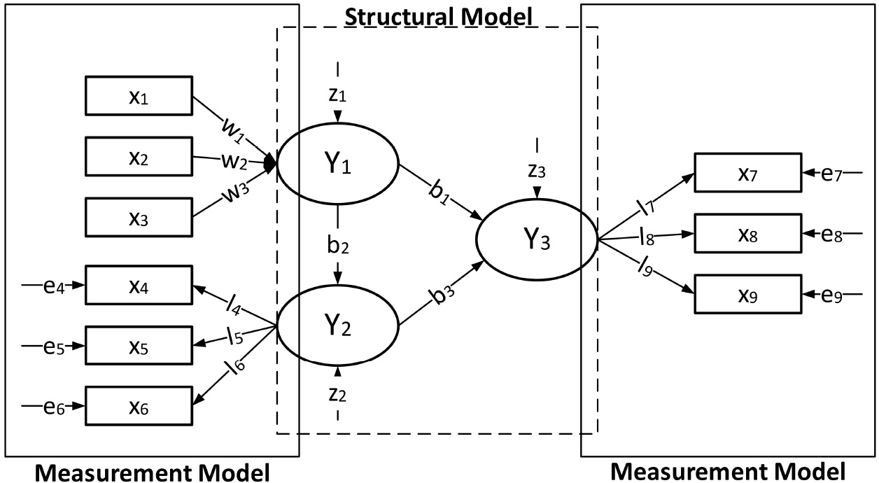

3.1.1 Structural model

The Structural Model is also called the internal model, and it consists of the arrangement of constructs and their relationship. The internal model represents the hypotheses and their relationships with the theory being tested, based on the researcher’s literature, logic, and practical experiences, which requires knowledge of the domain in which the study is being conducted. The organization of the structural model is an important tool for discussing ideas between researchers and domain experts, and should be prepared as one of the initial steps of a research [22].

In the model, independent variables, or predictors, or even exogenous latent variables, are arranged to the left ( $Y_{1}$ , in Fig. 1) and dependent variables, or endogenous latent variables, are arranged to the right of the model ( $Y_{3}$ , in Fig. 1). Dependent variables receive arrows that start from independent variables, and those that operate as both independent and dependent are represented in the middle of the diagram ( $Y_{2}$ , in Fig. 1).

Once the sequence of constructs has been defined, the relationships between them are then represented as arrows pointing to the right, indicating that the constructs on the left predict the constructs on the right. Causal relationships must be grounded in theory. The strength of the relationship between the constructs is indicated by coefficients ( $b_{1}$ to $b_{3}$ , in Fig. 1), calculated by the regression of each endogenous latent variable in its direct predecessor construct. The variance tha is not captured is also represented ( $z_{1}$ to $z_{3}$ in Fig. 1) [22, 45].

3.1.2 Measurement model

A measurement model represents the relationship between the latent variable and its indicators. How the constructs are measured must be well grounded in theory. The direction of the arrows informs the contribution of the indicators to the construct: reflective or formative.

A reflective model represents the effects or manifestations of a given construct. This kind of effect is indicated by arrows whose direction starts from the construct ( $Y_{2}$ and $Y_{3}$ in Fig. 1) to the indicators ( $x_{4}$ to $x_{9}$ in Fig. 1). In this type of model, the indicators can be understood as a significant sample of all items available in the construct’s conceptual domain, and they are highly correlated to each other. The reflective indicators relate to the construct as follows Eq. (1):

$\displaystyle x=lY+e,$ (1)

being $x$ the indicator coefficient, $Y$ is the construct coefficient, $l$ is the outer loading (calculated as the regression coefficient) that measures the strength of the relationship between $x$ and $Y$ , and $e$ measures the random error [45].

In the formative model, the direction of the arrows starts from the indicators to the construct ( $Y_{1}$ in Fig. 1), that combine linearly to form the construct. The outer weights ( $w_{1}$ to $w_{3}$ , in Fig. 1) indicate the strength of this relationship. The formative indicators relate to the construct as follows Eq. (2):

$\displaystyle Y=\sum_{k=1}^{K}w_{k}\cdot x_{k}+z,$ (2)

where $w_{k}$ is the outer weight of the $k$ indicator $(k=1,\cdots,K)$ to the construct $Y$ and $z$ represents the error associated with the construct $Y$ [45].

The contribution of formative indicators to the construct must be differentiated as causal or as composite. In the constructs measured by causal indicators, an error measure must be added, indicating that causes not considered can contribute to the construct’s formation [22].

3.1.3 PLS-SEM

In addition to contributing resources for constructing a path model representing the relationship between variables, SEM has instruments for deducting the interaction between variables themselves and between variables and their indicators. Among these instruments, the Partial Least Squares Structural Equation Modeling (PLS-SEM) statistical method is widely used in the exploratory multivariate data analysis in Social Sciences, Accounting, Health Care, Business, Management Information Systems, Supply Chain Management, Tourism, and Marketing [51, 56, 23, 3].

PLS-SEM utilizes sample data to estimate the contribution of variables and the strength of their relationships in an SEM model, seeking to minimize the unexplained residual variance of dependent variables. The PLS-SEM algorithm calculates and uses the coefficients of the latent variables ( $Y_{1}$ to $Y_{3}$ , in Fig. 1) as proxies for the indicators coefficients. The coefficients of the exogenous latent variables (predictors) are estimated as exact linear combinations of their indicators’ values. The resulting combination captures most of the variance of these indicators and predicts the endogenous indicators variables [45]. As an example, in Fig. 1 the value of the latent variable $Y\textsubscript{1}$ is calculated as a linear combination of the indicators $x\textsubscript{1}$ , $x\textsubscript{2}$ and $x\textsubscript{3}$ .

The PLS-SEM algorithm could be represented as in Algorithm 3.1.3.

[h] Initialization Stage 1: iterative calculation of weights (b1 to b3, in Fig. 1) and latent variables coefficients ( $Y_{1}$ to $Y_{3}$ , in Fig. 1) not converging Step 1: Internal weights $b_{ji}=\begin{cases}\textit{cov}(Y_{j};Y_{i})&\text{if $Y_{j}$ and $Y_{i}$ are% adjacent}\\ 0&\text{other cases}\end{cases}$ Step 2: Internal approximation $\tilde{Y}_{j}=\sum_{i}b_{ji}Y_{i}$ Step 3: External weights $\tilde{Y}_{jn}=\sum_{kj}\tilde{w}_{k_{j}}x_{k_{j}n}+d_{jn}$ (Mode A) $x_{kjn}=\tilde{w}_{k_{j}}\tilde{Y}_{jn}+e_{k_{j}n}$ (Mode B) Step 4: External approximation ${Y}_{jn}=\sum_{kj}\tilde{w}_{k_{j}}x_{k_{j}n}$ Stage 2: Calculation of external weights (w1 to w3, in Fig. 1), external loads (l4 to l9, in Fig. 1) and latent variables coefficients (Y1 to Y3, in Fig. 1)

PLS-SEM algorithm. Adapted from [24, 33].

As presented by [33], the PLS-SEM algorithm is initiated by the preliminary definition of the coefficients of the latent variables, assigning a weight of 1 (one) to all the indicators of the measurement model (line 3.1.3 of Algorithm 3.1.3). In practice, the algorithm performs Step 4 of Stage 1 (line 3.1.3 of Algorithm 3.1.3), calculating the coefficients of the latent variables by the sum of the product of the normalized coefficient ( $x_{k_{j}n}$ ) by the weight ( $\tilde{w}_{k_{j}}$ ) (arbitrarily set to 1) of your indicators.

Stage 1 estimates the internal weights ( $b_{1}$ to $b_{3}$ ) and the coefficients of the latent variables ( $Y_{1}$ to $Y_{3}$ ) using a four-step iterative procedure (lines 3.1.3 to 3.1.3 of Algorithm 3.1.3). In Step 1 of Stage 1 (line 3.1.3 of Algorithm 3.1.3) the internal weights ( $b_{ji}$ ) are calculated by the covariance between the normalized coefficients of the dependent latent variables ( $Y_{j}$ ), or endogenous, and the normalized coefficients of the independent latent variables ( $Y_{i}$ ), or exogenous. The internal weight will be 0 (zero) for unconnected latent variables.

In Step 2 of Stage 1 (line 3.1.3 of Algorithm 3.1.3) the coefficients of the latent variables are updated based on the new internal weights obtained from Step 1. For the exogenous latent variables $Y_{i}$ (Y1 and Y2, in Fig. 1) the new coefficient will be obtained by the product of the coefficient of the endogenous variable $Y_{j}$ (Y3, in Fig. 1) by the weight of the relationship with the exogenous variable $Y_{i}$ (b1 or b3, in Fig. 1). As an example, in Fig. 1 the new values of $Y_{1}$ and $Y_{2}$ will be obtained by $Y_{1}=Y_{3}\cdot b_{1}$ and $Y_{2}=Y_{3}\cdot b_{3}$ . Still in Step 2, the new coefficients of the endogenous latent variables $Y_{j}$ (Y3, in Fig. 1) will be calculated as the sum of the product between the coefficients of the latent variables exogenous $Y_{i}$ (Y1 or Y2, in Fig. 1) and the weights of the relationships with the endogenous variable $Y_{j}$ (b1 or b3, in Fig. 1). As an example, in Fig. 1 the new coefficient of the variable $Y_{3}$ is calculated as $\tilde{Y}_{3}=Y_{1}\cdot b_{1}+Y_{2}\cdot b_{3}$ . The new coefficients of the exogenous and endogenous latent variables are then normalized.

In Step 3 of Stage 1 (line 3.1.3 of Algorithm 3.1.3), new weights ( $w_{1}$ to $w_{3}$ and $l_{4}$ to $l_{9}$ , in Fig. 1) are calculated for the measurement model indicators (x1 to x9, in Fig. 1) indicating the strength of the relationship of indicators with latent variables. For the calculation the PLS-SEM algorithm uses two estimation modes: Mode A, used by default in reflective relationships (for example, $Y_{2}$ in relation to $x_{4}$ , $x_{5}$ and $x_{6}$ in Fig. 1), and Mode B, used by default in formative relationships (for example, $Y_{1}$ in relation to $x_{1}$ , $x_{2}$ and $x_{3}$ in Fig. 1). In Mode A (reflective) the loads ( $l_{4}$ to $l_{9}$ , in Fig. 1) are obtained as the bivariate correlation between each indicator and the latent variable. In Mode B (formative) the weights ( $w_{1}$ to $w_{3}$ , in Fig. 1) are obtained by regressing each latent variable in its indicators. In the lines 3.1.3 and 3.1.3 of Algorithm 3.1.3 $x_{k_{j}n}$ represents the data for the $k$ indicators $(k=1,\cdots,K)$ of latent variables $j(j=1,\cdots,J)$ and observations $n(n=1,\cdots,N)$ , $\tilde{Y}_{jn}$ represents the coefficients of the latent variables obtained in Step 2, $\tilde{w}_{k_{j}}$ are the external weights obtained in Step 3, $d_{jn}$ represents the error term of the bivariate regression and $e_{k_{j}n}$ represents the error term of the multiple regression.

The Step 4 of Stage 1 (line 3.1.3 of Algorithm 3.1.3) linearly combines the weights $\tilde{w}_{k_{j}}$ and the coefficients $x_{k_{j}n}$ of the indicators, obtained in Step 3, to calculate the coefficients of the latent variables ${Y}_{jn}$ , normalizing the values at the end of the calculation. The Stage 1 ends when the weights obtained in Step 3 show little variation from one iteration to the next (variation of $1\times 10^{-7}$ ) or when the maximum number of iterations is reached (by default, 300).

In Stage 2 the weights of the latent variables ( $b_{1}$ to $b_{3}$ , in Fig. 1) are calculated using the regression-based ordinary least squares method (OLS) based on the coefficients of the latent variables calculated on Stage 1 [24]. The weights of the latent variables ( $b_{1}$ to $b_{3}$ , in Fig. 1) will correspond to the linear regression coefficients. The coefficient of determination ( $R^{2}$ ) is also returned in this Step, and will correspond to the final value of the coefficient of the endogenous latent variable ( $Y_{3}$ , in Fig. 1). The coefficient of determination ( $R^{2}$ ) can be interpreted as the percentage of variance explained by the independent constructs that affect the dependent construct [24, 22, 33].

3.1.4 Path model evaluation

The objective of the PLS-SEM algorithm is to predict hypothetical relationships between constructs to maximize the explained variance of the dependent constructs ( $R^{2}$ ). The path model is evaluated by the discrepancy between its coefficients and the predicted values by the model, i.e., the path model’s predictive potential. The evaluation measures are separated between those that evaluate the structural model and those that evaluate the measurement model [22].

The PLS-SEM results validation follows a procedure consisting of three stages: starting with the validation of the reflective measurement model, going through the validation of the formative measurement model, and, if there is support for the quality of the measurement, reaching the validation of the structural model. The validation procedure is described in the next three subsections, following explanations and limits provided by [22, 45].

3.1.5 Reflective measurement model validation

In a reflective measurement model each indicator that measures a latent variable, or construct, represents one effect or manifestation of that construct. For this reason, indicators are expected to have a high correlation with each other. The way in which these indicators are evaluated takes into account the fact that they are correlated, but must ensure that they do not measure the same phenomenon.

The reflective measurement model is evaluated by examining the indicator’s loads ( $l_{4}$ to $l_{9}$ , in Fig. 1). PLS-SEM algorithm calculates the reflective indicators loadings as the bivariate correlation between each indicator and the latent variable. The square of a outer loading represents how much of the variation in this indicator is explained by the construct. As a rule of thumb, standardized values for outer loadings above 0.708 indicate that the latent variable explains more than 50% (or 0.708 ${}^{2}$ ) of the indicator’s variance, a satisfactory degree of reliability [22, p.103].

To ensure that reflective indicators of a latent variable have closely related outer loadings, the composite validity (or internal consistency reliability) of the indicators is calculated. The composite validity measures the inter-correlation between indicators of the same reflective latent variable, and its bounds are calculated at the lower limit by the Cronbach’s Alpha $\alpha$ index (Eq. (3)) and at the upper limit, by the composite reliability index $\rho_{c}$ (Eq. (4)) [21, p.15]:

$\displaystyle\alpha=\frac{K\cdot\bar{r}}{[1+(K-1)\cdot\bar{r}]},$ (3)

where $K$ corresponds to the number of latent variable indicators and $\bar{r}$ represents the not redundant average of the indicator correlation coefficient, and

$\displaystyle\rho_{c}=\frac{(\sum_{k=1}^{K}l_{k})^{2}}{(\sum_{k=1}^{K}l_{k})^{% 2}+\sum_{k=1}^{K}\textit{var}(e_{k})},$ (4)

where $l_{k}$ indicates the standardized value of the indicator load $k$ of a construct with $K$ indicators, $e_{k}$ represents the measurement error of the indicator $k$ and $\textit{var}(e_{k})$ represents the measurement error variance, calculated as $\textit{var}(e_{k})=1-l_{k}^{2}$ . Acceptable values for $\alpha$ and $\rho_{c}$ are, respectively, 0.60 to 0.90, that indicate increasing degrees of reliability [22, p.101].

Convergent validity is the extent to which an indicator correlates positively with alternative indicators for the same construct. As reflective indicators are treated as different approaches to measuring the same construct, indicators must converge or share a high proportion of variance. A standard measure of convergent validity is the Average Variance Extracted (AVE) (Eq. (5)):

$\displaystyle\text{AVE}=\frac{(\sum_{k=1}^{K}l_{k})^{2}}{K},$ (5)

where $l_{k}$ is the loading of indicator $k$ of a construct measured by $K$ indicators. Values of 0.5 or greater indicate that the construct explains more than half of its indicators’ variance [22, p.103].

Discriminant validity can be understood as the extent to which a construct is, in fact, distinct from other constructs by empirical standards. If the discriminant validity is established, that construct is unique and captures a phenomenon not represented by other constructs in the model. Discriminant validity is measured by examining the cross loads of the indicators (i.e., a load of an item in one construct must be greater than its load in other constructs). Another measuring is the Fornell-Larcker criterion, which establishes that the square root of the AVE of each latent variable must be greater than a more significant correlation between latent variables [22, p.105].

3.1.6 Formative measurement model validation

In a formative measurement model each indicator that measures a latent variable, or construct, captures a specific aspect of the construct’s domain. For this reason, indicators are combined linearly to form the construct, and the outer weights ( $w_{1}$ to $w_{3}$ , in Fig. 1) indicate the strength of each relationship. PLS-SEM algorithm calculates the formative indicator’s weights by regressing each construct in its indicators. So, formative measurement model’s assessment requires different instruments from those used in assessing the reflective measurement model.

The first instrument is the verification of the convergent validity, which in the context of formative constructs will ensure that the complete domain of the construct and all its facets have been covered by the adopted indicators. The convergent validity of formative constructs is determined as the extent to which this construct correlates with another reflective construct that captures the same concept. This procedure requires the prior inclusion of reflective indicators in research and data collection phases [22, p.121]. In the case of current research, it is assumed that the proposed formative construct is completely covered by its indicators, since the research was limited to measuring the construct only by the indicators most commonly found in the literature (Section 3.1.2).

As they capture different aspects of the construct, it is not expected to find a high correlation between the formative indicators. High correlations in formative indicators are called collinearity, which can be measured by the variation inflation factor (VIF) index in each indicator of the formative latent variables. The VIF index (Eq. (6)) calculation consists of applying a multiple regression of each indicator to all other indicators of the same latent variable:

$\displaystyle\textit{VIF}_{k}=\frac{1}{1-R_{k}^{2}},$ (6)

where $R_{k}^{2}$ corresponds to the coefficient of determination of the $k$ -th regression, for the calculation of the VIF index of the $k$ -th indicator. High values of $R^{2}$ suggest that the indicator’s variance can be explained by the other indicators of the same construct, configuring the indicator’s collinearity. Values above 5 indicate the collinearity of indicators [22, p.126], but ideally they should be close to 3 or lower [21, p.10].

The final step is assessing each indicator’s relative contribution to the latent variable’s construction. Normalized values of the indicators’ weights close to 0 indicate weak relationships, and values close to 1 or $-$ 1 represent strong relationships. However, the statistical significance of the weights must be assessed. As explained in Algorithm 3.1.3, the weights of the formative indicators are calculated as a result of a multiple regression in which the construct acts as the dependent variable and the formative indicators act as independent variables. Although the weights of formative indicators can be compared to assess their relative contribution to the construct, their truly contribution must be validated. The bootstrapping procedure allows testing whether the weights of formative indicators are significantly different from zero. The bootstrapping consists in the construction of subsamples based on the original data, used to estimate the model. The process is repeated multiple times until the significance of the indicator weights can be validated [22, p.127].

The bootstrapping procedure allows the computation of standard errors and the significance of the indicator weight [48]. If the weight of the indicator is statistically significant, the indicator is maintained. If the indicator’s weight is not statistically significant, but its load is equal to or greater than 0.50, the indicator can be maintained with adequate evidence to support this. The indicator must be removed if the weight is less than 0.50 and there is no statistical significance of the weight. In the case of various formative indicators and the presence of some statistically insignificant weights, the indicators should be grouped into other constructs if there is theoretical support [24].

3.1.7 Structural model validation

After completing the measurement models’ evaluation, the structural model is evaluated for problems of collinearity between latent variables and for its predictive capacity. The assessment of collinearity problems in constructs uses the same instrument used in assessing the collinearity in indicators of formative constructs, the VIF index, with the difference that instead of indicators, the equation’s input will be the exogenous latent variables. VIF values greater than five will indicate collinearity between the latent predictive variables [45].

As for assessing the model’s predictive capacity, three criteria must be considered: the determination coefficient $R^{2}$ , the cross-validation redundancy $Q^{2}$ , and the model coefficients. The coefficient of determination $R^{2}$ indicates the variance explained in the endogenous latent variables, meaning the accuracy of the predictive model. In general, values of 0.75, 0.50, and 0.25 are considered, respectively, substantial, moderate, and weak; however, the context of the analysis must be considered. Another validation of the structural model is called the Stone-Geisser $Q^{2}$ , which measures the predictive relevance of the model by an iterative process of “blindly” omitting data points from reflective latent variable indicators or endogenous latent variables with only one indicator to verify whether the PLS-SEM algorithm accurately predicts the missing points using the remaining points. The missing points are treated by the PLS-SEM algorithm as missing values, being replaced by the mean criterion [22]. If the predicted value is close to the real one, with a low prediction error, the model will have high predictive accuracy.

Finally, but no less important is the validation of the weights of the relationships between the latent variables, whose standardized values vary between $-$ 1 and $+$ 1. Values close to $+$ 1 or $-$ 1 indicate strong relationships, which in general are statistically significant. The closer the weights are to 0, the weaker the relationships will be. However, the bootstrapping procedure will allow obtaining the standard error and calculating the empirical $t$ value. To estimate the significance of the relationship between the latent variables $Y_{1}$ and $Y_{3}$ in Fig. 1 the calculation to be made is (Eq. (7)):

$\displaystyle t=\frac{b_{1}}{se_{b_{1}}^{*}}$ (7)

where $b_{1}$ corresponds to the weight of the relationship between the latent variables $Y_{1}$ and $Y_{3}$ in Fig. 1, and $se_{b_{1}}^{*}$ corresponds to the standard error of the weight $b_{1}$ obtained by the bootstrapping method. The quantiles of a normal distribution can be used as critical values against which the $t$ -value will be compared. Commonly used values are 1.65 (10% significance level), 1.96 (5% significance level) and 2.57 (1% significance level). In exploratory studies, a significance level of 10% can be assumed. $p$ -value is also used in conjunction with $t$ -value as an indicator of the significance of the relationship between two latent variables [22].

As previously presented, Structural Equation Modeling seeks to find a relationship between dimensions of latent variables that are represented by indicators that, in fact, measure the model. Since this paper aims to relate indicators of Data Quality and Data Complexity concerning the impact on Classification Quality, in the next subsections these dimensions will be discussed, and the indicators to be adopted in this work will be presented.

3.2 Data quality

Data Quality (DQ) is a vast concept in the literature that can have different meanings in each step of the Data Analysis pipeline, starting from data collection to its transformation for analytical purposes [34, 53, 30]. In this work context, DQ can be defined as the level of confidence and precision that the data found so that applying an analytical method can be trusted.

In the literature of KDD, several works have shown the effect of currency, accuracy, completeness, consistency, and timeliness of data on tasks of data mining as association rules and data classification [7, 8, 20]. For the specific case of data classification, that is the interest of this work, outliers and missing values problems are appointed as the main DQ indicators [20].

The accounting of outliers could be measured through the Validity indicator proposed by [30]. The validity of a dataset $p$ is calculated based on the proportion of extreme data points on the complete dataset and can be represented as:

$\displaystyle V_{p}=1-\left(\frac{n}{N}\right),$ (8)

where $N$ is the number of objects in the dataset $p$ and $n$ is the number of extreme data objects. For the identification of extreme objects, the Mahalanobis distance could be applied, adopting $\chi^{2}$ with $d$ degrees of freedom as a threshold, $d$ being the number of attributes of the dataset [1, p.243].

The missing values could be measured by the Completeness indicator, which supposes the randomness of the generation process of missing values (Missing Completely at Random, MCAR). An observation with a missing value will be classified as MCAR when any other object is equally likely to contain a missing value [14]. The Completeness of a set $p$ can be calculated based on the proportion of missing values on the complete dataset [8] and can be represented as:

$\displaystyle C_{p}=1-\left(\frac{n}{N(1+A)}\right),$ (9)

where $N$ is the number of objects of the dataset $p$ , $A$ is the number of attributes, and $n$ is the number of missing values.

Table 1

Data complexity categories and indicators. Adapted from [17]

Indicator	Definition
Feature-based measures
F1	Maximum Fisher’s Discriminant Ratio
F1v	Directional-vector Maximum Fisher’s Discriminant Ratio
F2	Volume of overlap region
F3	Feature efficiency
F4	Collective feature efficiency
Neighborhood measures
N1	Fraction of Borderline Points
N2	Ratio of Intra/Extra Class Nearest Neighbor Distance
N3	Error Rate of the Nearest Neighbor Classifier
N4	Non-Linearity of the Nearest Neighbor Classifier
N5	Fraction of Hyperspheres Covering Data
N6	Local Set Average Cardinality
Linearity measures
L1	Sum of the Error Distance by Linear Programming
L2	Error Rate of Linear Classifier
L3	Non-Linearity of a Linear Classifier
Dimensionality measures
D1	Average number of points per dimension
D2	Average number of points per PCA dimension
D3	Ratio of the PCA Dimension to the Original Dimension
Balance measures
B1	Entropy of class proportions
B2	Imbalance Ratio
Structural representation
G1	Average density of the network
G2	Clustering coefficient
G3	Hub score

3.3 Data Complexity

Data Complexity (DC) in KDD can be defined as the way data is distributed and the level of overlap between objects of different classes. The DC indicators proposed in the literature and of interest in this present research are presented by [37], based originally on [26, 36], and summarized in Table 1 under four categories: Feature-based measures, Neighborhood measures, Linearity measures, Dimensionality measures, Class balance measures, and Structural representation measures.

3.3.1 Feature-based measures

Feature-based measures assess the discriminating power of data attributes, treating datasets that have at least one discriminating attribute as less complex [25]. The first measure is Maximum Fisher’s Discriminant Ratio ( $F1$ ), which measures the overlap between the values of different class attributes and can be applied to binary or multi-class ratings. The calculation of $F1$ presented by [37] already gives normalized results, indicating that values close to 1 represent datasets with few discriminating attributes and, therefore, more complex. Directional-vector maximum Fisher’s discriminant ratio ( $F1v$ ) is complementary to $F1$ , looking for a vector that separates the two classes after the data points are projected on it. The higher the value of $F1v$ , the less complex the dataset [37, p.3]. The measure volume of the overlapping region ( $F2$ ) calculates the distributions overlap of the values of the attributes within the classes. For each attribute, minimum and maximum values are obtained in the classes, and the overlapping region is then calculated and normalized by the value range of both classes. Maximum individual feature efficiency ( $F3$ ) estimates each attribute’s efficiency in separating the classes, considering the highest value found among the attributes. There is an overlap between classes for each attribute, considering them ambiguous in the region where there is an overlap. A problem is considered simple if there is at least one attribute that has low ambiguity between classes. To that extent, the higher the value, the simpler the problem. Collective feature efficiency ( $F4$ ) successively applies a procedure similar to that adopted in $F3$ . Initially, the most discriminating attribute is identified, apost which all objects that that attribute can separate are eliminated. The procedure is repeated until all attributes have been considered and there are no objects that can be eliminated. The result of $F4$ is calculated by the rate of data points that have not been discriminated in relation to the total number of data points. Higher values of $F4$ indicate a less complex problem.

3.3.2 Linearity measures

The measures in the linearity category attempt to quantify the possibility of separating classes by a Support Vector Machine-based hyperplane, assuming that a linearly separable problem is less complex than a problem requiring a non-linear decision limit [37]. The first measure, the sum of the error distances by linear programming ( $L1$ ), computes the linear separability of classes by the sum of the distances of the objects classified incorrectly in relation to the hyperplane used for their separation. In a linearly separable problem, this sum is zero. The measure error rate of a linear classifier ( $L2$ ) computes the SVM linear classifier’s error rate. Finally, the measure non-linearity of a linear classifier ( $L3$ ) calculates the error rate of a linear classifier tested on a dataset generated from data points of the original dataset. Each exemplar in the test set is obtained by linear interpolation of two exemplars in the same class, chosen randomly from the original dataset.

3.3.3 Neighborhood measures

The neighborhood measures attempt to characterize the class overlap, capturing the shape of the decision region and the classes’ internal structure by analyzing the neighborhood of the points. The distances between pairs of points are stored in a matrix, measured by the Gower distance. The first measure, fraction of borderline points ( $N1$ ), estimates the complexity and size of a decision region needed to separate objects from different classes. A Minimum Spanning Tree (MST) is built from the original data, where each vertex corresponds to a data point and the edges are weighted according to the distance between the points. The value of $N1$ represents the percentage of vertices incident to edges connecting data points of opposite classes in the MST. The measure ratio of intra/extra class nearest neighbor distance ( $N2$ ) calculates the ratio between the sum of the distances between each object and its closest neighbor in the same class and the sum of each object and its closest neighbor from another class. Smaller values for this measure indicate less complex problems. The measure error rate of the nearest neighbor classifier ( $N3$ ) refers to the error rate of the k-Nearest Neighbors classifier for $k=1$ , estimated by the leave-one-out procedure. The measure non-linearity of the nearest neighbor classifier ( $N4$ ) is similar to the $L3$ measure, except that it uses the kNN classifier instead of a linear predictor. High values for $N4$ indicate high complexity. The measure fraction of hyperspheres covering data ( $N5$ ) computes the ratio between the number of hyperspheres and the total number of data points in the dataset. The hyperspheres are constructed as proposed by [37]. The smaller the number of hyperspheres covering the data, the less complex this dataset is, indicating that the same class’s data are densely distributed and close to each other. Finally, for the calculation of the local measure set average cardinality ( $N6$ ) local sets are considered, which are groups of data points of a dataset whose distance to another sample is less than the distance of that object for your closest enemy.

3.3.4 Structural representation measures

In structural representation measures, the dataset is represented as a graph, preserving the distances or similarities between the original data points. In this graph, the vertices correspond to the objects, connected by edges weighted by the objects’ distance. The distances between pairs of points, measured by the Gower distance, are stored in a matrix. The process includes pruning the edges between data points of different classes. The first measure of this category, average density of the network ( $G1$ ), considers the number of edges retained in the graph constructed from the dataset normalized by the maximum number of edges between $n$ data pairs. Low values for this measure indicate dense regions of the same class’s connected points, corresponding to lower complexity. The clustering coefficient measure ( $G2$ ) is calculated as the ratio of the number of edges of neighbors to a vertex $v_{i}$ and the maximum number of edges that could exist between them. Less complex datasets, with denser regions of connections between the same class data points, will have lower values for $G2$ . The hub score measure ( $G3$ ) calculates the influence of nodes in the graph by assigning an index to each vertex, based on its connections with other vertices and based on the number of connections from its neighbors. In datasets with high class overlap, the vertices will be less connected to strong neighbors, increasing the value of $G3$ .

3.3.5 Dimensionality measures

Dimensionality measures indicate the sparsity of the data based on the size of the dataset. The first indicator, the average number of points per dimension ( $D1$ ), reflects the sparsity of the dataset by calculating the ratio between the dimensionality and the set of points in the dataset. Less sparse datasets indicate less complex problems. The second indicator, the average number of points per PCA dimension ( $D2$ ), estimates the sparsity of the dataset by calculating the average number of points per Principal Component Analysis (PCA) component needed to represent 95% of the variability of the data. The last indicator of this category, the ratio of the PCA dimension to the raw dimension ( $D3$ ), estimates the proportion of dimensions relevant to the dataset. The higher the value of $D3$ , the more attributes are needed to describe the data’s variability, and the more complex the dataset will be.

3.3.6 Class balance measures

Finally, the last category, class balance measures, groups together measures that capture significant differences in the number of exemplars per class, which indicate more complex problems. The first measure, the entropy of class proportions ( $B1$ ), estimates class imbalance by calculating the normalized entropy of class size distribution. The higher the value of $B1$ , the more balanced the classes will be. The measure imbalance ratio ( $B2$ ) estimates class balance by calculating the average number of classes in a dataset.

3.4 Classification quality

Classification is the Data Mining task that models a dataset’s grouping structure using the objects of a dataset. The most popular classification models are decision-trees, rule-based classifiers, probabilistic models, instance-based classifiers, support vector machines, and neural networks [1]. For the present research, some algorithms were selected that do not require previous treatment of data quality problems: C4.5, CART, and Random Forests. As evidenced by the KDD process’s pre-processing step, missing values and outliers tend to reduce dataset analyses’ quality. However, it remains to be seen how these problems affect the C4.5, CART, and Random Forests data classification models.

Decision tree algorithms are based on a tree structure built based on training data to classify new objects. In this tree, the internal nodes correspond to attribute tests, the branches correspond to test results, and the leaves represent the classes. An induction algorithm determines the most appropriate choice for a node, and some of the classic induction algorithms are C4.5, ID3, and CART. C4.5 is a decision tree induction algorithm that uses information as a criterion for deciding the tree breaking attribute. In the decision tree’s induction, missing values are considered in the nodes’ construction, either treating them as a possible branch or distributing these occurrences between the branches respecting the distribution of data utilizing weights. At the time of classification, missing data causes each branch of the node corresponding to the attribute to be tested [43]. On the other hand, outliers can lead the process of inducing overfitting of the tree to the data, requiring algorithms that handle the overfitting [50].

Another tree-based algorithm is CART (Classification And Regression Trees), which uses the Gini index to decide the tree’s breaking attribute. The CART algorithm ignores occurrences with missing values in measuring the quality of a break and uses surrogate splits to determine how to deal with missing values in the test step of the classification [16]. As in the C4.5 algorithm, trees induced by the CART algorithm require treatment to avoid overfitting. As for the effect of outliers on the CART algorithm, the literature argues that the CART algorithm is not significantly affected by outliers in independent variables but is affected locally by outliers present in the dependent variables [28, p.552][40, p.161].

Random Forests (RF) is a class of tree-based classification methods that apply the bootstrapping method to the dataset to decrease the prediction variance. The predictions of multiple trees are combined to present the classification model. Random Forests are resistant to noise and discrepancies of independent variables because they apply the binning method’s normalization to the variables [1, p.381]. In the original definition of Random Forests by [11], missing values are treated by imputation. Random Forests implementations using C4.5 decision trees instead of CART take the C4.5 algorithm approach to deal with missing values.

Table 2 summarizes the behavior of the classification algorithms used in the present research in the face of missing values and outliers. The research initially chose not to use algorithms that required previous treatment of outliers and missing values by imputing data or deleting objects.

4. Experimental methodology

4.1 Proposed structural and measurement models

Literature provides the elements that support a proposition of a path model in which Classification Quality is affected by the complexity and the quality of data. Nevertheless, both Data Quality and Data Complexity are concepts whose observation is not direct. Thus, for a SEM analysis, these concepts have to be defined as constructs or latent variables. Each construct is measured indirectly through indicators that manifest themselves as quality and complexity dimensions. For structural modeling, the constructs need to be conceptually defined. Thus, this work has opted for an adaptation of complexity definition by Kolgomorov (1965) to Data Complexity [26, 9] and Data Quality following the Jayawardene definition [30]. Consequently, the constructs that are the focus of this research can be defined as follows:

•
Data Complexity (DC) – Necessary effort to describe a dataset. The greater the effort, the more complex are the data;
•
Data Quality (DQ) – Fidelity with which data represent people, objects, events, or concepts. The bigger the quality, the closer the proximity between the representation and the object or fact represented;
•
Classification Quality (CQ) – Effectiveness with which the non-labeled objects are classified correctly. The bigger the quality, the closer the proximity of labeled objects to their correct classes.

From these definitions, the relation between constructs can be initially modeled as in Fig. 2.

Table 2
Behavior of the classification algorithms used in the search for missing values and outliers

Algorithm Missing values Outliers

C4.5 Handles missing values Handles outliers, requiring algorithms to avoid overfitting

CART Handles missing values Not significantly affected by outliers in independent variables, but affected locally

by outliers in dependent variables

RF Handles missing values Handles outliers

Figure 2.
Proposed models of path and measurement of constructs.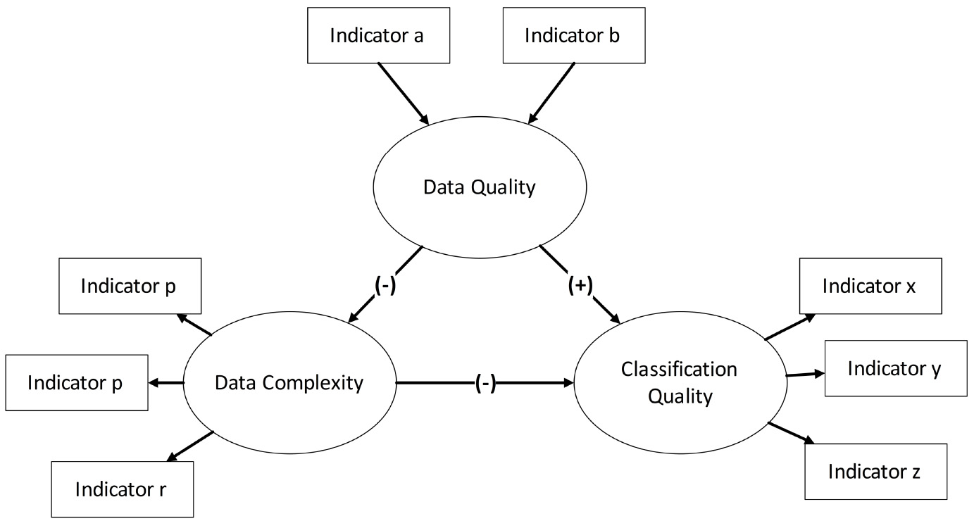

In Fig. 2, it is possible to note from the signs that the construct Data Quality (DQ) has a positive effect ( $+$ ) on the Classification Quality (CQ) and a negative effect ( $-$ ) on Data Complexity (DC). The positive effect, represented by ( $+$ ), can be understood as a positive correlation between two constructs, and the negative effect, represented by ( $-$ ), can be understood as a negative correlation. So this representation hypothesizes: the lower the Data Complexity, the higher the quality of the classifier results, and the higher the Data Quality, the lower its complexity, and the higher the quality of the classifier results.

These effects were noted, for instance, by [35] when observing that outliers (a quality dimension) affect the data in its variance-dependent dimensions, such as overlapping measures (complexity dimensions), which may in turn affect the result of classifiers (classification dimensions) such as Decision Trees and Support Vector Machines.

The model for measuring the constructs, shown in Fig. 2, was theoretically based on the literature presented in Subsections 3.2 and 3.3. The indicators of the Data Quality construct (Indicators a and b) are Completeness and Validity. For the Data Complexity construct, the data complexity dimensions presented in Table 1 correspond to Indicators p, q, and r. The results of the classifiers listed in Table 2 correspond to Indicators x, y, and z.
4.2 Experimental dataset

Algorithm	Missing values	Outliers
C4.5	Handles missing values	Handles outliers, requiring algorithms to avoid overfitting
CART	Handles missing values	Not significantly affected by outliers in independent variables, but affected locally
		by outliers in dependent variables
RF	Handles missing values	Handles outliers

The approach adopted to obtain the experimental dataset, based on [26], was to build a space for measures of Data Complexity and Data Quality for data classification problems, where the attributes are the Data Quality, Data Complexity and Classification Quality indicators, obtained for public datasets. It was of interest to the researchers to know the effect of data containing outliers and missing values not submitted to pre-processing on classification algorithms’ results. Thus, the experiments predicted a dataset’s constitution that contained classification results for datasets containing outliers and untreated missing values.

The experimental dataset’s size is directly related to statistical power, that is, the probability of rejecting a null hypothesis when it is false. By adopting a dataset with missing values, the statistical power is reduced, and there is a risk of compromising a data distribution that is assumed to have with the complete data [38, p.34]. To calculate the sample size for PLS-SEM algorithm, the following values were assumed, as suggested by [22, pp.20-22]: minimum size of the effect detected as significant (0.3), statistical power (80%) and level of significance (5%).

4.3 Attributes and data points

The attributes of the dataset are the following: a) the dimensions of Data Complexity presented in Table 1, b) Validity and Completeness, calculated as described in Eqs (8) and (9), and c) the AUC values (Area Under the ROC Curve) representing the performance of the classification algorithms in Table 2. The AUC represents the degree of separability, that is, how much an algorithm is able to distinguish between the classes, and its measurement varies between [0, 1]. For the calculation of AUC, the ROCR package [46] was used, applied to each of the classification algorithms in Table 2, using the cross-validation method in k-folders, for $k=10$ . To calculate the complexity dimensions, the ECoL package [18] was used. For the identification of extreme points, the Mahalanobis function was used, implemented in the R by stats package [41], adopting $p=0.95$ and $\chi^{2}$ with $d$ degrees of freedom as threshold, $d$ being the number of attributes of the dataset. The tolerance of $1\mathrm{e}{-20}$ has been defined as the maximum limit for the function solve to assume very small values as zero. The experimental dataset attributes are shown in Table 3.

Table 3
Experimental dataset attributes

Attribute	Description	Data type	Domain
datasetName	Dataset name	Categorical	*
MDAttributes	Number of dataset attributes	Discrete	[2, 20]
MDElements	Number of dataset data points/exemplars	Discrete	[100, 3000]
DQMissingValues	Number of missing values in dataset	Discrete	$\geqslant 0$
DQOutliers	Number of outliers in dataset	Discrete	$\geqslant 0$
DQCompleteness	Dataset completeness (Eq. (9))	Continuous	[0, 1]
DQValidity	Dataset validity (Eq. (8))	Continuous	[0, 1]
B1	Entropy of class proportions	Continuous	[0, 1]
B2	Imbalance Ratio	Continuous	[0, 1]
D1	Average number of points per dimension	Continuous	$\geqslant 0$
D2	Average number of points per PCA dimension	Continuous	$\geqslant 0$
D3	Ratio of the PCA Dimension to the original dimension	Continuous	[0, 1]
F1	Maximum Fisher’s Discriminant Ratio	Continuous	[0, 1]
F1v	Directional-vector Maximum Fisher’s Discriminant Ratio	Continuous	[0, 1]
F2	Volume of overlap region	Continuous	[0, 1]
F3	Feature efficiency	Continuous	[0, 1]
F4	Collective feature efficiency	Continuous	[0, 1]
L1	Sum of the Error Distance by Linear Programming	Continuous	[0, 1]
L2	Error Rate of Linear Classifier	Continuous	[0, 1]
L3	Non-Linearity of a Linear Classifier	Continuous	[0, 1]
N1	Fraction of Borderline Points	Continuous	[0, 1]
N2	Ratio of Intra/Extra Class Nearest Neighbor Distance	Continuous	[0, 1]
N3	Error Rate of the Nearest Neighbor Classifier	Continuous	[0, 1]
N4	Non-Linearity of the Nearest Neighbor Classifier	Continuous	[0, 1]
N5	Fraction of Hyperspheres Covering Data	Continuous	[0, 1]
N6	Local Set Average Cardinality	Continuous	[0, 1]
G1	Average density of the network	Continuous	[0, 1]
G2	Clustering coefficient	Continuous	[0, 1]
G3	Hub score	Continuous	[0, 1]
C4.5	AUC for C4.5 algorithm	Continuous	[0, 1]
RF	AUC for Random Forests algorithm	Continuous	[0, 1]
CART	AUC for Classification And Regression Trees algorithm	Continuous	[0, 1]

Considering the 27 attributes for the experimental dataset (22 dimensions of Data Complexity, 2 dimensions of Data Quality, and 3 dimensions of Classification Quality), the minimum sample size necessary to detect the effect was calculated as 119 exemplars [22, p.21][47].

To obtain the values for the experimental dataset’s attributes, this work searched in OpenML repository [13] for datasets that met the following criteria: number of instances between 100 and 3,000, number of attributes between 2 and 20, number of classes equal to 2, number of missing values equal to or greater than 0. The rationale why binary datasets (2 classes) have been adopted is that a majority of complexity measures are defined for binary classification problems only. However, multi-class problems can be decomposed into binaries by the OVO (One-vs-One) strategy [37]. The number of attributes was defined considering that the dimensionality of the dataset affects its complexity [25, 26, 35, 44, 19, 55, 5]. The number of missing values defined in the selection criterion aimed at obtaining mixed datasets, with and without missing values. The range for the number of instances has been set arbitrarily.

After applying the criteria, 178 datasets were obtained from the OpenML repository. The datasets that were redundant and had problems with data were deleted. From these 178 datasets, metadata were collected to build the space for measures of complexity and data quality for classification problems.

5. Results and discussions

5.1 Descriptive analysis

A complete descriptive analysis of the experimental dataset was carried out. For the reasons related to space, only the results of the quality attributes of the classification will be presented.

As for the Classification Quality construct indicators, the classifiers’ AUC measures presented in Table 2 were adopted. The selected classification algorithms are sensitive to missing values and outliers, capturing these anomalies’ variations in the analyzed datasets.

The summary measures for the classification quality indicators are:

C4.5 RF CART

Min. :0.4833 Min. :0.3605 Min. :0.4420

1st Qu.:0.6582 1st Qu.:0.6778 1st Qu.:0.6508

Median :0.8033 Median :0.8410 Median :0.8084

Mean :0.7724 Mean :0.7969 Mean :0.7714

3rd Qu.:0.9069 3rd Qu.:0.9296 3rd Qu.:0.8677

Max. :1.0000 Max. :1.0000 Max. :1.000

By observing the summary, these classifiers’ desirable performance can be seen in 50% of the analyzed datasets. The frequency distribution of the classifiers C4.5, RF, and CART indicators can be seen in Fig. 3.

Figure 3.

Histogram for classification quality indicators.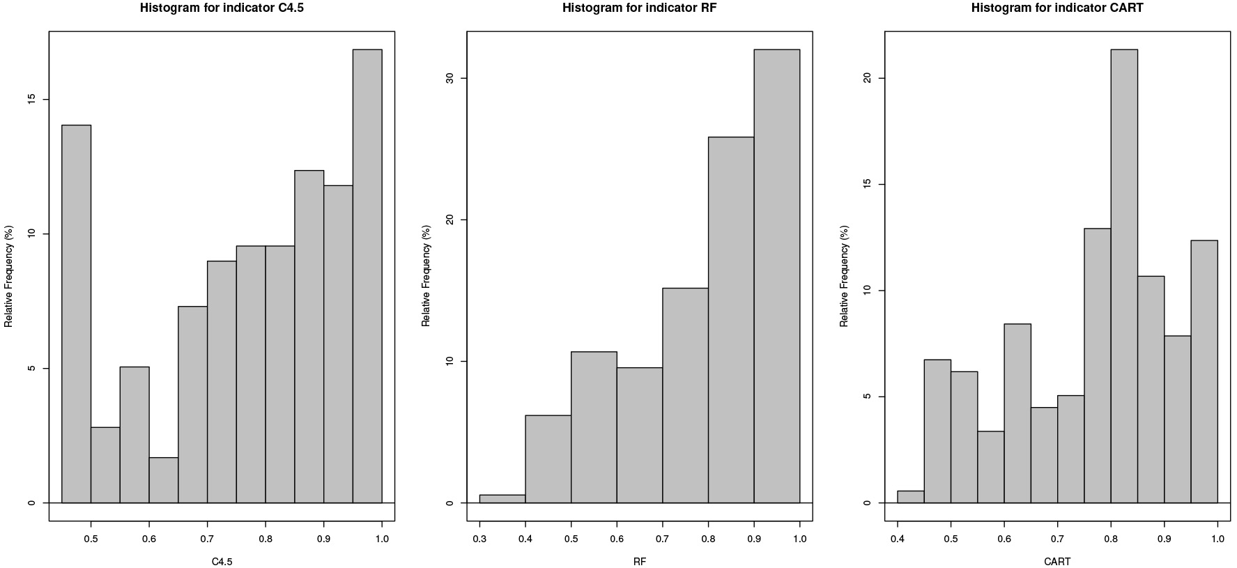

The correlation between the indicators was calculated as:

C4.5 RF CART

C4.5 1.0000000 0.8626815 0.8608670

RF 0.8626815 1.0000000 0.9287369

CART 0.8608670 0.9287369 1.000000

For the indicators of the Classification Quality construct, the value of Cronbach’s alpha coefficient as well as the gain of reliability in case of exclusion of any of the indicators, are presented below:

Alpha reliability = 0.9571

Standardized alpha = 0.9581

Reliability deleting each item in turn:

Alpha Std.Alpha r(item, total)

C4.5 0.962 0.963 0.878

CART 0.926 0.926 0.927

RF 0.923 0.925 0.927

A Cronbach’s alpha value of 0.958 is considered a high-reliability value for the Classification Quality construct’s measurement model [22, p.101].

The evaluation of the PLS-SEM algorithm results begins by validating the reflective and formative measurement models’ quality. Only if the measurement characteristics of the constructs are acceptable can the results of the structural model be validated [22, p.101].

5.2 Reflective model validation

The evaluation of the reflective model begins with assessing the reliability of the internal consistency of the constructs. For this evaluation, Cronbach’s alpha measure $\alpha$ and the composite reliability index $\rho_{c}$ are used, whose results are presented in the Table 4.

Table 4
Reflective constructors reliability

	Cronbach’s alpha $\alpha$	Composite reliability $\rho_{c}$
Data Complexity	0.889	0.918
Classification Quality	0.958	0.973

Although high values for composite reliability $\rho_{c}$ indicate higher degree of reliability, satisfactory values are between 0.70 and 0.90. Values above 0.90 are not desirable since they occur when the construct’s indicators are redundant [22, p.102].

The researchers opted to retain the Data Complexity construct as it is, with an expectation to reduce the redundancy in measures through the elimination of the indicators with much clearer guidelines. As for the Classification Quality construct, the research opted for maintaining the three indicators in Table 2, considering that: a) indicator removal simulations did not show any significant gain in the values of Cronbach’s alpha and composite reliability; b) although the three algorithms adopted, CART, C4.5, and Random Forests, are based on trees and their classification performances are close, the permanence of their measures in the analysis is justified by the fact that it deals with different algorithms and since no other classification algorithms are found that are both sensitive to outliers and missing values.

The next stage of analysis of the reflective constructs consists of measuring the convergent validity of each construct’s indicators, that is, a measure of how much the indicator is positively correlated with other indicators of the same construct. For this evaluation, loads of the indicators and the Average Variance Extracted (AVE) are considered. Although standardized values of 0.708 or greater are expected for the indicator loads, [22, pp.103,104] recommend considering the impact of excluding an indicator with a load between 0.40 and 0.708 on the Average Variance Extracted and on the composite reliability.

The values for loads of the Data Complexity and Classification Quality constructs’ reflective indicators are presented in Table 5.

Table 5

Loads of the Data Complexity and Classification Quality constructs’ reflective indicators

Data Complexity
Indicator	Load
B1	$-$ 0.271
B2	$-$ 0.253
D1	0.012
D2	0.046
D3	0.222
F1	0.728
F1v	0.792
F2	0.414
F3	0.776
F4	0.737
G1	0.811
G2	0.399
G3	$-$ 0.007
L1	0.850
L2	0.878
L3	0.880
N1	0.893
N2	0.708
N3	0.873
N4	0.767
N5	0.793
N6	0.750
Classification Quality
RF	0.971
C4.5	0.939
CART	0.971

It is possible to note that the Classification Quality construct indicators showed high commonality, being kept unchanged. However, some Data Complexity construct indicators presented loads below 0.40 (bold lines in Table 5). The researchers chose to exclude the indicators D1, D2, D3, G2, and G3, evaluating the exclusion of gains in composite reliability and the AVE for each exclusion. After this exclusion, loads of indicators B1 and B2 (indicators of class unbalance) remained negative. The research option was based on exclusion of indicators B1 and B2. The results for reliability and validity are shown in Table 6.

Table 6

Reliability and validity for reflective constructs after exclusion of indicators D1, D2, D3, G2, G3, B1, and B2

	Cronbach’s alpha $\alpha$	Composite reliability $\rho_{c}$	AVE
Data Complexity	0.956	0.961	0.625
Classification Quality	0.958	0.973	0.923

The values for loads of the Data Complexity and Classification Quality constraints’ reflective indicators after the exclusions of indicators D1, D2, D3, G2, G3, B1, and B2 are shown in Table 7.

Table 7

Loads of the Data Complexity and Classification Quality constraints’ reflective indicators after the exclusions of indicators D1, D2, D3, G2, G3, B1, and B2

Indicator	Load
Data Complexity
F1	0.699
F1v	0.810
F2	0.438
F3	0.770
F4	0.755
G1	0.817
L1	0.875
L2	0.905
L3	0.896
N1	0.887
N2	0.702
N3	0.873
N4	0.764
N5	0.783
N6	0.762
Classification Quality
RF	0.971
C4.5	0.939
CART	0.972

Although high, the values of reliability and validity were considered acceptable for the analysis, considering that: a) the research has only three indicators to measure the Classification Quality, representing the few classification algorithms sensitive to values outliers and missing values; b) the different aspects of the data complexity discussed by [37] were summarized in just one latent variable; c) the AVE values for the constructs are above 0.5, being considered acceptable [22, p.107].

Finally, the analysis of reflective constructs involves assessing their discriminant validity, that is, how different the construct is from other constructs. For this validation, the cross loads of the indicators are analyzed, which must be greater than all their loads in other constructs, and the results of the Fornell-Larcker [22, p.105] criterion.

The values for the cross loads of the indicators are presented in Table 8.

Table 8

Reflective indicators’ cross loads (highlighted in bold) of Data Complexity (DC) and Quality of Classification (CQ) constructs

Indicator	DC	CQ
F1	0.699	$-$ 0.505
F1v	0.810	$-$ 0.648
F2	0.438	$-$ 0.054
F3	0.770	$-$ 0.499
F4	0.755	$-$ 0.407
G1	0.817	$-$ 0.431
L1	0.875	$-$ 0.566
L2	0.905	$-$ 0.574
L3	0.896	$-$ 0.565
N1	0.887	$-$ 0.692
N2	0.702	$-$ 0.477
N3	0.873	$-$ 0.737
N4	0.764	$-$ 0.599
N5	0.783	$-$ 0.470
N6	0.762	$-$ 0.373
RF	$-$ 0.672	0.971
C4.5	$-$ 0.575	0.939
CART	$-$ 0.708	0.972

The values of the discriminant analysis by the Fornell-Larcker criterion are presented in Table 9.

Table 9

Values of the discriminant analysis by the Fornell-Larcker criterion for reflective constructs

	Data Complexity	Classification Quality
Data Complexity	0.791
Classification Quality	$-$ 0.682	0.961
Data Quality	0.051	0.118

It is possible to conclude by the results of cross loads and the values of the discriminant analysis with the Fornell-Larcker criterion that the Quality of Classification and Data Complexity constructs are different from each other, that is, they measure different phenomena.

5.3 Formative model validation

The validation of the formative model followed the steps evaluating different aspects of the reflective model.

The first instrument for the validation of the formative model is verifying convergent validity. Convergent validity is the extent to which the formative construct correlates with another reflective construct of a single item that captures the same concept but uses different indicators. The reflective construct of a single global item that captures the same concept is defined in the design phase of research in Social Sciences, but does not exist in the present research because all the data quality attributes that are of interest in the research form the Data Quality construct.

The second instrument used to validate the formative model is the collinearity of its indicators, that is, a high correlation between them. Since formative indicators measure different aspects of the construct’s phenomenon, a high correlation between them is not anticipated. The VIF indicator (Variance Inflation Factor) measures the degree to which the standard error increases due to the presence of collinearity. For collinearity values that are considered as non-critical (VIF $<5$ ), the significance of the weights and the contribution of the indicator must be analyzed [22, pp.125,126].

The validation of the formative model involves evaluating the indicator’s contribution, expressed by its weight. In addition to being compared with each other to calculate their relative contribution, the weights of the indicators are tested by the bootstrapping approach to see if they are significantly different from zero. For the execution of bootstrapping, 5,000 sub-samples were generated ( $\alpha=0.05$ , two-tailed test).

The values of collinearity, original weights, and significance after bootstrapping observed for the Data Quality construct’s formative indicators are shown in Table 10.

Table 10
Collinearity, weight, and significance values for the indicators of the Data Quality construct

Indicator	VIF	Weight	$t$ -value	Confidence interval
DQCompleteness	1.002	0.993	1.999	[0.0189; 1.9671]
DQValidity	1.002	0.162	0.348	[ $-$ 0.7494; 1.0734]

For the DQCompleteness indicator, the weight of 0.993 was considered significantly different from zero, at a significance level of 0.05, for the two-tailed test. For the DQValidity indicator, the weight of 0.162 was considered insignificant, at a significance level of 0.05, for the two-tailed test. However, it was decided to maintain the DQValidity indicator to keep the construct domain compatible with the theory.

5.4 Structural model validation

In this step, the structural model representing the relationship between Data Quality, Data Complexity, and Classification Quality are validated. The results allow understanding how well the empirical data supports the structural model’s concepts and verify whether these concepts have been empirically confirmed.

The initial analysis step is the search for collinearity in the structural model, which is identified with VIF values above 5. The next step aims to validate the significance and relevance of the structural model’s relationships. Then follows the evaluation of the explained variance ( $R^{2}$ ) and the effect size ( $f^{2}$ ). These measures assess the predictive capacity of the structural model [22, p.169].

Table 11 presents the results and indicators significance of the relationships proposed by the structural model.

Table 11
Results and significance indicators of the relationships proposed by the structural model. DC stands for Data Complexity constructor, DQ stands for Data Quality constructor, and CQ stands for Classification Quality constructor. SD stands for standard deviation

Relationship	VIF	$f^{2}$	Standardized structural coefficient	SD	$t$ -value	$p$ -value	$Q^{2}$	Adjusted $R^{2}$
$DC\rightarrow CQ$	1.003	0.930	$-$ 0.690	0.038	18.08	0.000	0.438	0.483
$DQ\rightarrow CQ$	1.003	0.046	0.154	0.097	1.59	0.113	0.438	0.483
$DQ\rightarrow DC$	1.000	0.003	0.051	0.086	0.60	0.552	0.001	0.003

The values presented in Table 11 indicate that no collinearity was observed in the sets of predictor variables. The standardized structural coefficients’ values represent the coefficients of the relationships between the constructs, with a standardized value ranging between $-$ 1 and 1. The values of the standardized structural coefficient observed for the relationship of the Data Quality construct with the Classification Quality construct (0.154) along with the Data Complexity construct (0.051), indicate weak relationship, stating that they are not significant since their $t$ -values are 1.59 and 0.60, respectively, for a significance level of 5%. The relationship between the Data Complexity and Classification Quality constructs has a standardized coefficient of $-$ 0.690 with a $t$ -value of 18.08, with a significance level of 5%.

The adjusted $R^{2}$ values represent the combined effects of the exogenous constructs on the endogenous constructs along with the variance in the endogenous constructs explained by the endogenous constructs connected to them. The results presented in Table 11 inform that the Data Quality construct explained only 0.3% of the variance of the Data Complexity construct. In contrast, the Data Quality and Data Complexity constructs explained 48.3% of the variance of the Classification Quality construct. The value of $Q^{2}$ , obtained by the blindfolding process with an omission distance of 7 units, confirms the model’s predictive relevance to predict the points of the Classification Quality construct.

Figure 4 shows the paths between the constructs, highlighted proportionally about their contribution to the result of the endogenous construct. The values of arrows connecting the constructs represent the partial regression coefficients between the dependent and the independent constructs. The values of arrows that link the DQCompleteness and DQValidity indicators to the Data Quality construct represent the multiple regression coefficients between these indicators and the construct. The values that appear on the arrows that link the indicators to the Data Complexity and the Classification Quality constructs represent the simple regression coefficients between each indicator and the construct. The $t$ -values are represented in parentheses.

5.5 Applicability

Knowing the proportion as CQ is affected by DQ and DC allows anticipating the result of a classification analysis, based on the results of the dataset’s quality and complexity indicators. Before submitting a dataset for analysis, it is possible to collect the Data Quality and Data Complexity indicators to show the trend of the classification task’s result: high values for Data Complexity indicators may suggest an unsatisfactory performance for classifiers in this dataset.

The contribution of the model of relationships between Data Complexity, Data Quality and Classification Quality generated by the PLS-SEM algorithm is to allow a more accurate estimate of the influence of data quality and complexity on the final result of classification quality.

An example of application of the structural model presented in Fig. 4 can be the generation of a radar chart, like the one presented in Fig. 5. In this chart, four datasets from the OpenML repository [13] were submitted to the data quality and complexity metadata collection procedures described in the Sections 3.2 and 3.3. It is possible to represent the collected indicators directly on the chart, or group them into categories before the graphical representation.

In Fig. 5, the Data Quality and Data Complexity indicators were grouped, and the new values were calculated by weighted average of the indicators loads and weights, represented in Fig. 4 (Table 12).

Table 12
Calculation of grouped measures of Data Complexity and Data Quality, by weighted average criterion. The weights were obtained from the model generated by the PLS-SEM algorithm (Fig. 4)

Measure	Interpretation	Calculation (weighted average of indicators)
Feature	Attempt to assess the discriminating power of data attributes. Datasets that have at least one discriminating attribute are less complex [25]	$(F10.699)+(F1v0.810)+(F20.438)+(F30.770)+(F4*0.755))/(0.699+0.810+0.438+0.% 770+0.755)$
Neighborhood	Attempt to characterize the class overlap, capturing the shape of the decision region and the classes’ internal structure by analyzing the neighborhood of the points [37]	$(N10.887)+(N20.702)+(N30.873)+(N40.764)+(N50.783)+(N60.762))/(0.887+0.70% 2+0.873+0.764+0.783+0.762)$
Linearity	Attempt to quantify the possibility of separating classes by a Support Vector Machine-based hyperplane. A linearly separable problem is less complex than a problem requiring a non-linear decision limit [37]	$(L10.875)+(L20.905)+(L3*0.896))/$ $(0.875+0.905+0.896)$
Structural	Attempt to extract structural complexity from a graph that represents the dataset [37]	$(G1*0.755)/(0.755)$
Data Quality	Combina as medidas de qualidade de dados: completude e validade (Section 3.4)	$(\textit{DQCompleteness}0.993)+(\textit{DQValidity}0.162))/$ $(0.993+0.162)$

Figure 4.

Structural model showing paths, weights and loads, and 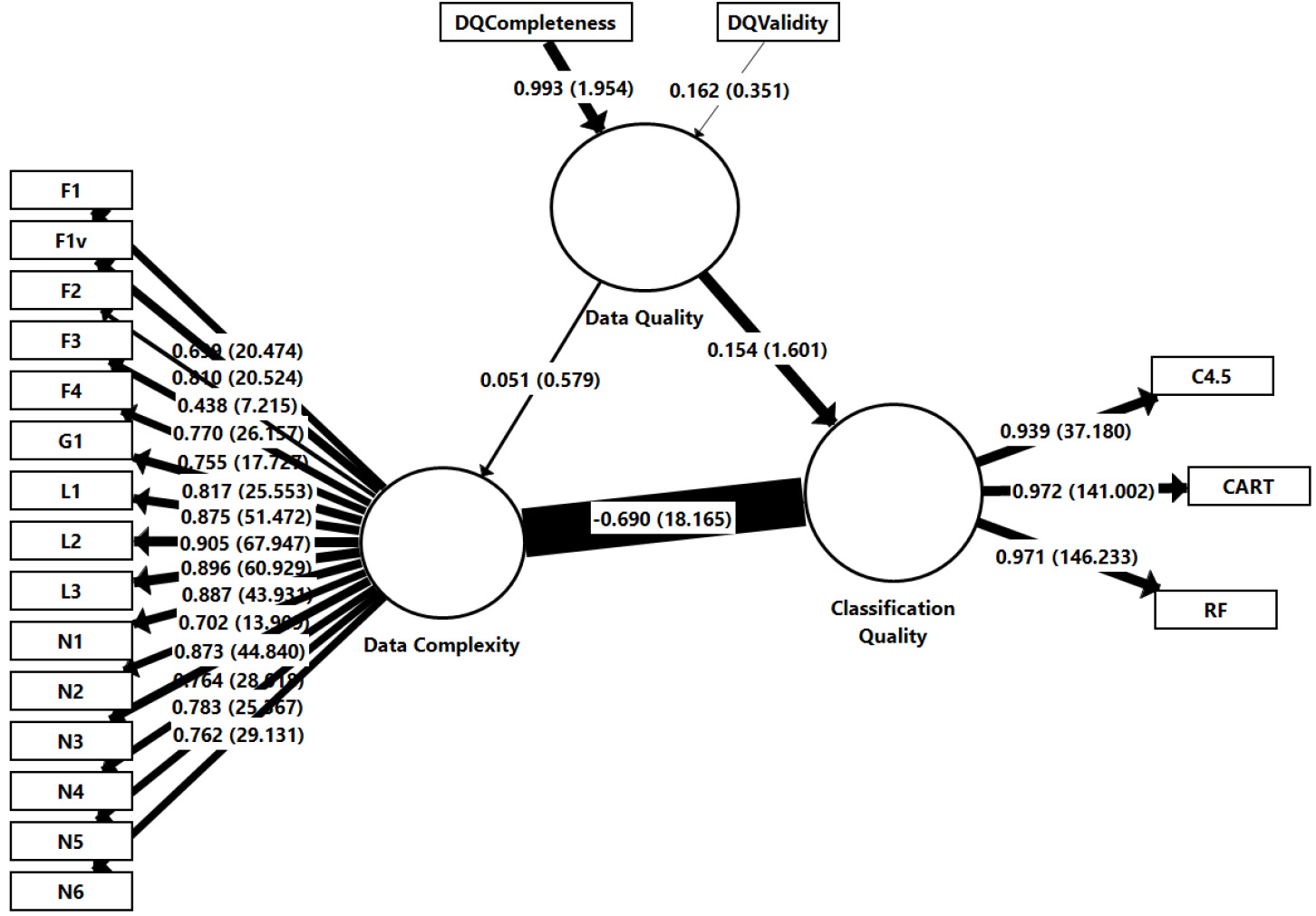$t$ -values. Source: Author.

Figure 5.

Graphical representation of Data Quality and Data Complexity measures. Source: Author.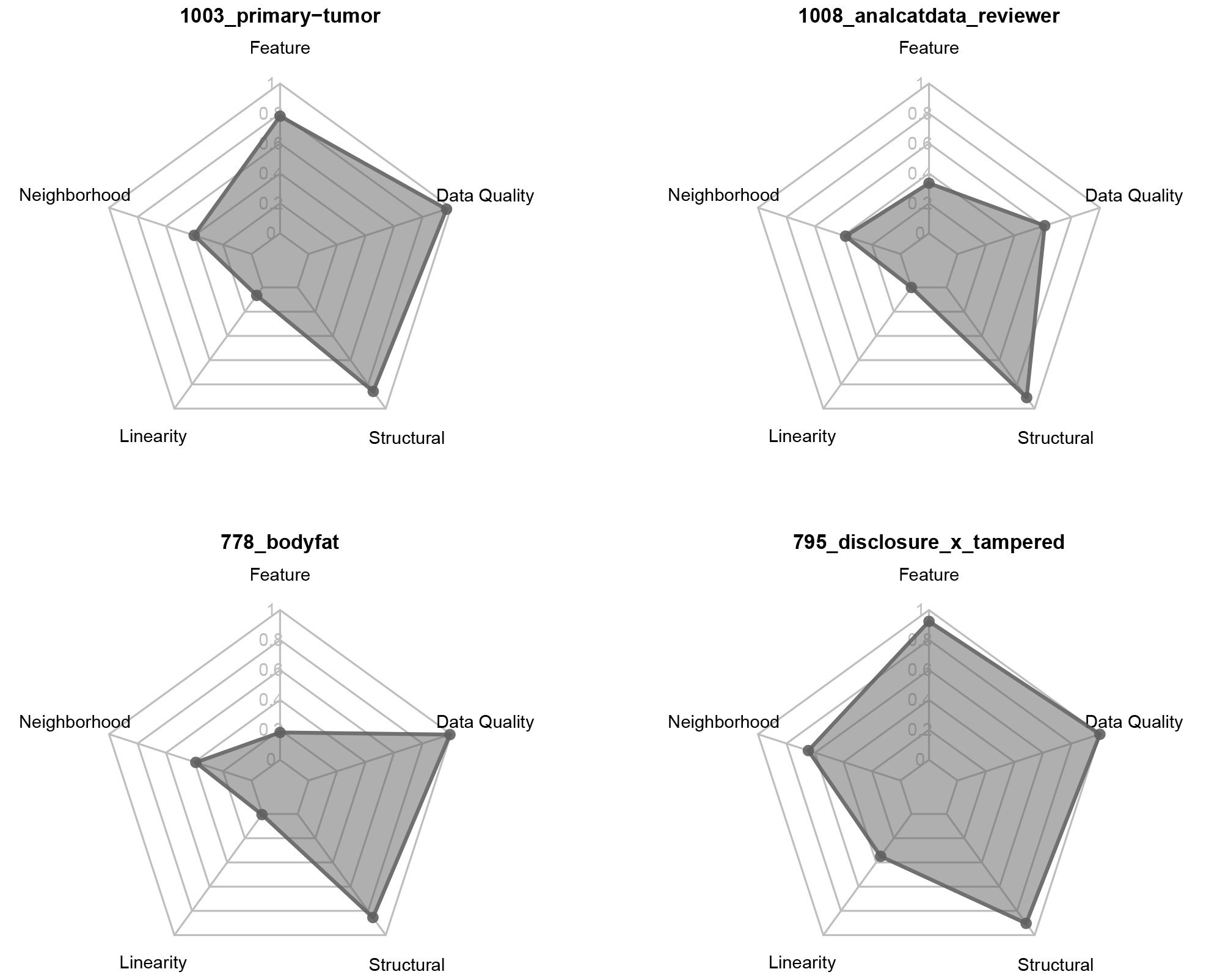

The graphical representation of the clustered measures of data complexity and quality can be interpreted from the results of the PLS-SEM process (Section 5.4): data complexity exerts a strong negative impact (0.690) on quality of the classification results. Together, the complexity and quality of the analyzed data can explain approximately 48% of the variation in classification results. In simpler terms: the greater the complexity of the data and the lower its quality, and the worse the classification results for that data.

6. Conclusions and further work

Data quality is a real and well-represented concern in the process of Knowledge Discovery in Databases. A better understanding regarding the relation of Data Quality and Data Complexity may bring quality gains to analyses, which should not be ignored in a Big Data reality.

The research proved itself to be innovative by relating data aspects that, in general, are treated separately and whose effect is nearly ignored: Data Quality affects Data Complexity, and both affect Classification Quality. Validity and completeness were shown in the current model as two vital quality problems whose effect on Data Complexity deserves to be studied more thoroughly. Besides, the use of Structural Equation Modeling and the PLS-SEM algorithm for studying the relations between quality and complexity dimensions, to the best of our knowledge, is unprecedented in literature, and it has opened a new platform for this tooling in the areas of Data Mining, Big Data, and Data Governance.

PLS-SEM’s use allowed for the quantification of the combined contribution of data quality and complexity to the success of classifications in the datasets of two classes. The results suggest that the structural factors that interfere in a dataset’s complexity deserve more attention in classification problems than the occurrence of missing values and outliers, and this requires a greater investment of time by the analyst in the pre-processing steps.

As a continuation of the research, it is suggested that the study of the relationship between Data Quality and Data Complexity be deepened, including new indicators to verify the impact on the relationships discovered in this work. Besides, it is also intended to think of other works to validate the application of the model discovered in this research. The resulting model allows, among other things, to know a priori the types of problems that a dataset has and the classifier’s probable performance in case no corrective action is taken. In this sense, it is suggested to research the proposed model’s use to recommend corrective actions that reduce datasets’ pre-processing time in analyzes.

References

Aggarwal

C.C.

, Data Mining, Springer International Publishing, 2015.

Auer

and Felderer

, Addressing data quality problems with metamorphic data relations, in: 2019 IEEE/ACM 4th International Workshop on Metamorphic Testing (MET), IEEE, may 2019.

Avkiran

N.K.

, Rise of the partial least squares structural equation modeling: An application in banking, in: Partial Least Squares Structural Equation Modeling, pages 1–29, Springer International Publishing, 2018.

Azeroual

and Jha

, Without data quality, there is no data migration, Big Data and Cognitive Computing 5(2) (2021).

Barella

V.H.

Garcia

L.P.

de Souto

M.P.

Lorena

A.C.

and De Carvalho

, Data complexity measures for imbalanced classification tasks, in: 2018 International Joint Conference on Neural Networks (IJCNN), pages 1–8, IEEE, 2018.

Basu

and Ho

T.K.

, Data Complexity in Pattern Recognition, Springer London, Londres, Reino Unido, 2006.

Berti-Equille

, Data quality awareness: A case study for cost optimal association rule mining, Knowledge and Information Systems 11(2) (2007), 191.

Blake

and Mangiameli

, The effects and interactions of data quality and problem complexity on classification, Journal of Data and Information Quality 2(2) (feb 2011), 1–28.

Boschetti

, Mapping the complexity of ecological models, Ecological Complexity 5(1) (2008), 37–47.

10.

Bosu

M.F.

and Macdonell

S.G.

, Experience: Quality benchmarking of datasets used in software effort estimation, Journal of Data and Information Quality 11(4) (sep 2019), 1–38.

11.

Breiman

and Cutler

, Random forests, https://www.stat.berkeley.edu/∼breiman/RandomForests/, 2004. Accessed February 09, 2021.

12.

Cano

J.R.

, Analysis of data complexity measures for classification, Expert Systems with Applications 40(12) (2013), 4820–4831.

13.

Casalicchio

Bossek

Lang

Kirchhoff

Kerschke

Hofner

Seibold

Vanschoren

and Bischl

, Openml: An r package to connect to the machine learning platform openml, Computational Statistics 32(3) (2017), 1–15.

14.

Davey

et al., Statistical power analysis with missing data: A structural equation modeling approach, Routledge, 2009.

15.

Fayyad

Piatetsky-Shapiro

and Smyth

, From data mining to knowledge discovery in databases, AI Magazine 17(3) (1996), 37–37.

16.

Feelders

, Handling missing data in trees: Surrogate splits or statistical imputation? in: Principles of Data Mining and Knowledge Discovery, pages 329–334, Springer Berlin Heidelberg, 1999.

17.

Garcia

Lorena

and Lehmann

, ECoL: Complexity measures for classification problems, 2018.

18.

Garcia

Lorena

Souto

and Ho

T.K.

, ECoL: Complexity Measures for Supervised Problems, 2020. R package version 0.4.0.

19.

Garcia

L.P.

de Carvalho

A.C.

and Lorena

A.C.

, Effect of label noise in the complexity of classification problems, Neurocomputing 160 (2015), 108–119.

20.

Hair

J.F.

Black

W.C.

Babin

B.J.

and Anderson

R.E.

, Multivariate Data Analysis, Pearson Education Limited, 2014.

21.

Hair

J.F.

Risher

J.J.

Sarstedt

and Ringle

C.M.

, When to use and how to report the results of pls-sem, European business review, 2019.

22.

Hair

J.F.

Jr Hult

G.T.M.

Ringle

and Sarstedt

, A primer on partial least squares structural equation modeling (PLS-SEM), Sage publications, 2016.

23.

Hallak

and Assaker

, Using partial least squares structural equation modeling (PLS-SEM) in tourism research, in: Management Science in Hospitality and Tourism, pages 99–123, Apple Academic Press, mar 2017.

24.

Henseler

Ringle

and Sarstedt

, Using partial least squares path modeling in advertising research: basic concepts and recent issues, pages 252–276, Edward Elgar, 2012.

25.

T.K.

and Basu

, Measuring the complexity of classification problems, in: Proceedings 15th International Conference on Pattern Recognition. ICPR-2000, IEEE Comput. Soc.

26.

T.K.

and Basu

, Complexity measures of supervised classification problems, IEEE Transactions on Pattern Analysis and Machine Intelligence 24(3) (mar 2002), 289–300.

27.

T.K.

Basu

and Law

M.H.C.

, Measures of geometrical complexity in classification problems, in: Data Complexity in Pattern Recognition, pages 1–23, Springer, 2006.

28.

Härdle

W.K.

and Simar

, Applied Multivariate Statistical Analysis, Springer-Verlag Berlin Heidelberg, 4 edition, 2015.

29.

Januzaj

and Januzaj

, An application of data mining to identify data quality problems, in: 2009 Third International Conference on Advanced Engineering Computing and Applications in Sciences, IEEE, oct 2009.

30.

Jayawardene

Sadiq

and Indulska

, An analysis of data quality dimensions, ITEE Technical Report 2015(2) (2015), 35–43.

31.

Karkouch

Mousannif

Moatassime

H.A.

and Noel

, Data quality in internet of things: A state-of-the-art survey, Journal of Network and Computer Applications 73 (sep 2016), 57–81.

32.

Laranjeiro

Soydemir

S.N.

and Bernardino

, A survey on data quality: Classifying poor data, in: 2015 IEEE 21st Pacific Rim International Symposium on Dependable Computing (PRDC), IEEE, nov 2015.

33.

Latan

and Noonan

, Partial least squares path modeling: Basic concepts, methodological issues and applications, Springer, 2017.

34.

Liebenau

and Backhouse

, Understanding Information, Macmillan Education UK, 1990.

35.

Lorena

A.C.

and de Carvalho

A.C.

, Evaluation of noise reduction techniques in the splice junction recognition problem, Genetics and Molecular Biology 27(4) (2004), 665–672.

36.

Lorena

A.C.

and de Souto

M.C.

, On measuring the complexity of classification problems, in: International Conference on Neural Information Processing, pages 158–167, Springer, 2015.

37.

Lorena

A.C.

Garcia

L.P.

Lehmann

Souto

M.C.

and Ho

T.K.

, How complex is your classification problem? a survey on measuring classification complexity, ACM Computing Surveys (CSUR) 52(5) (2019), 1–34.

38.

McKnight

P.E.

McKnight

K.M.

Sidani

and Figueredo

A.J.

, Missing data: A gentle introduction, Guilford Press, 2007.

39.

Morán-Fernández

Bolón-Canedo

and Alonso-Betanzos

, Can classification performance be predicted by complexity measures? A study using microarray data, Knowledge and Information Systems 51(3) (2017), 1067–1090.

40.

Nisbet

Elder

and Miner

, Handbook of statistical analysis and data mining applications, Academic Press, 2009.

41.

R Core Team, R: A Language and Environment for Statistical Computing, R Foundation for Statistical Computing, Vienna, Austria, 2020.

42.

Rosli

M.M.

Tempero

and Luxton-Reilly

, Can we trust our results? a mapping study on data quality, in: 2013 20th Asia-Pacific Software Engineering Conference (APSEC), IEEE, dec 2013.

43.

Salzberg

S.L.

, C4.5: Programs for machine learning by j. ross quinlan. morgan kaufmann publishers, inc., 1993, Machine Learning 16(3) (sep 1994), 235–240.

44.

Sánchez

J.S.

Mollineda

R.A.

and Sotoca

J.M.

, An analysis of how training data complexity affects the nearest neighbor classifiers, Pattern Analysis and Applications 10(3) (2007), 189–201.

45.

Sarstedt

Ringle

C.M.

and Hair

J.F.

, Partial least squares structural equation modeling, Handbook of Market Research 26 (2017), 1–40.

46.

Sing

Sander

Beerenwinkel

and Lengauer

, ROCR: Visualizing classifier performance in r, Bioinformatics 21(20) (aug 2005), 3940–3941.

47.

Soper

D.S.

, A-priori sample size calculator for structural equation models [software], https://www.danielsoper.com/statcalc, 2017. Accessed February 17, 2021.

48.

Streukens

and Leroi-Werelds

, Bootstrapping and pls-sem: A step-by-step guide to get more out of your bootstrap results, European Management Journal 34(6) (2016), 618–632.

49.

Taleb

Serhani

M.A.

Bouhaddioui

and Dssouli

, Big data quality framework: A holistic approach to continuous quality management, Journal of Big Data 8(1) (may 2021).

50.

Tan

P.-N.

Steinbach

and Kumar

, Introduction to data mining, Pearson Education India, 2 edition, 2018.

51.

Tenenhaus

Vinzi

V.E.

Chatelin

Y.-M.

and Lauro

, Pls path modeling, Computational Statistics & Data Analysis 48(1) (2005), 159–205.

52.

Valverde

M.C.

Vallespir

Marotta

and Panach

J.I.

, Applying a data quality model to experiments in software engineering, in: Lecture Notes in Computer Science, pages 168–177, Springer International Publishing, 2014.

53.

Wang

R.Y.

and Strong

D.M.

, Beyond accuracy: What data quality means to data consumers, Journal of Management Information Systems 12(4) (mar 1996), 5–33.

54.

Wook

Hasbullah

N.A.

Zainudin

N.M.

Abdul Jabar

Z.Z.

Ramli

Razali

N.A.M.

and Yusop

N.M.M.

, Exploring big data traits and data quality dimensions for big data analytics application using partial least squares structural equation modelling, Journal of Big Data 8 (2021).

55.

Zubek

and Plewczynski

D.M.

, Complexity curve: A graphical measure of data complexity and classifier performance, PeerJ Computer Science 2 (2016), e76.

56.

Zwicker

Souza

C.A.d.

and Bido

D.d.S.

, Uma revisão do modelo do grau de informatização de empresas: novas propostas de estimação e modelagem usando pls (partial least aquares), in: Encontro da Associação Nacional de Programas de Pós-Graduação em Administração – ENANPAD, ANPAD, 2008.

Modeling the combined influence of complexity and quality in supervised learning

Abstract

Keywords

1. Introduction

2. Problem definition and literature review

3. Methodological formulation

3.1 Path model

3.1.2 Measurement model

3.1.4 Path model evaluation

3.1.5 Reflective measurement model validation

3.3.1 Feature-based measures

3.3.2 Linearity measures

3.3.3 Neighborhood measures

3.3.4 Structural representation measures

3.3.5 Dimensionality measures

3.3.6 Class balance measures

3.4 Classification quality

4. Experimental methodology

4.1 Proposed structural and measurement models

4.3 Attributes and data points

Table 3 Experimental dataset attributes

5.1 Descriptive analysis

Table 4 Reflective constructors reliability

Table 10 Collinearity, weight, and significance values for the indicators of the Data Quality construct

Table 11 Results and significance indicators of the relationships proposed by the structural model. DC stands for Data Complexity constructor, DQ stands for Data Quality constructor, and CQ stands for Classification Quality constructor. SD stands for standard deviation

Table 12 Calculation of grouped measures of Data Complexity and Data Quality, by weighted average criterion. The weights were obtained from the model generated by the PLS-SEM algorithm (Fig. 4)

References

Table 3
Experimental dataset attributes

Table 4
Reflective constructors reliability

Table 10
Collinearity, weight, and significance values for the indicators of the Data Quality construct

Table 11
Results and significance indicators of the relationships proposed by the structural model. DC stands for Data Complexity constructor, DQ stands for Data Quality constructor, and CQ stands for Classification Quality constructor. SD stands for standard deviation

Table 12
Calculation of grouped measures of Data Complexity and Data Quality, by weighted average criterion. The weights were obtained from the model generated by the PLS-SEM algorithm (Fig. 4)