
Abstract
As a research hotspot in ensemble learning, clustering ensemble obtains robust and highly accurate algorithms by integrating multiple basic clustering algorithms. Most of the existing clustering ensemble algorithms take the linear clustering algorithms as the base clusterings. As a typical unsupervised learning technique, clustering algorithms have difficulties properly defining the accuracy of the findings, making it difficult to significantly enhance the performance of the final algorithm. AGglomerative NESting method is used to build base clusters in this article, and an integration strategy for integrating multiple AGglomerative NESting clusterings is proposed. The algorithm has three main steps: evaluating the credibility of labels, producing multiple base clusters, and constructing the relation among clusters. The proposed algorithm builds on the original advantages of AGglomerative NESting and further compensates for the inability to identify arbitrarily shaped clusters. It can establish the proposed algorithm’s superiority in terms of clustering performance by comparing the proposed algorithm’s clustering performance to that of existing clustering algorithms on different datasets.
Introduction
Image processing, recommender systems, and data analysis all benefit from clustering analysis. It aims to divide data objects into classes with high intra-class similarity and low inter-class similarity. Numerous clustering methods have been designed from various perspectives to achieve this goal [33]. Han and Kamber [18] categorized these methods into partitioning, hierarchical, density-based, model-based, and grid-based methods.
This paper attempts to propose a strategy for integrating Multiple AGglomerative NESting algorithms (MAGNES). Cluster ensemble [29, 17] is a common methodology, which helps to combine multiple base clusterings to improve the prominence of the cluster results. However, the unsupervised nature of the clustering algorithm makes it difficult to integrate several base algorithms when the dataset is unlabeled, further improvements are still possible. According to the study of Bai et al. [5, 4]. There are three key elements that influence the effect of clustering ensemble:
Label credible evaluation. When a single algorithm completes, part of the data may have the wrong clustering labels. If the points are never classified correctly, then the validity of the final ensemble will be affected by the incorrect labels. How to correctly judge the credibility of the clustering labels is the key to improving the ensemble performance.
Inter-cluster dissimilarity of base clusters. In clustering integration, the base clustering algorithms should be distinct from each other to obtain more robust results. If the base clustering algorithms all have extremely similar outputs, then the integration operation will be meaningless. Therefore, Bai generated different multiple basis clusters by introducing the randomness of fuzzy k-means [5] and k-means [4] algorithms to obtain the best results.
Inter-cluster equivalence relations. Unlike classification algorithms that have independent labels, the same result may be reflected on different clustering labels. So it is necessary to determine which clustering labels have an equivalence relationship. A reasonable clustering relationship is a prerequisite for obtaining good clustering results. Since different base clusters generated by the same base clustering algorithm may also represent the same true classification, the inter-cluster equivalence relation should be the overall relation of all base clusters owned by different base algorithms.
To overcome these problems, Bai et al. [4] argued that a cluster center’s local space might be represented by that center. Based on this hypothesis, this paper uses AGglomerative NESting (AGNES) as a base clustering algorithm. By building a hypothetical center to construct the local space, this paper proposes a MAGNES algorithm with a well-clustered result.
The structure of this paper is as follows. Section 2 introduces the related research progress in the field of cluster ensemble. Section 3 covers the ideas linked to granulation methods and offers the MAGNESs ensemble structure. Section 4 shows the experimental assessment of the proposed ensemble structure and a summary. Section 5 concludes with recommendations for future improvements.
The two main steps in the ensemble technique are Generation and Consensus. Generation is the first step, where a set of different base clusterings are generated. There are some methods for generating a base clustering set, of which two methods are more efficient. The first one is a mechanism that combines several single algorithms with different parameters, different clustering algorithms, and different algorithms on several dataset subsets. The second is the “granulation” method based on the local hypothesis. Different from the first method, the second method introduces the concept of label credibility, which provides consistency, novelty, and stability.
Consensus is the second step, in which you must be proficient in enlightening the solitary clustering algorithm. Different consensus functions have been developed to derive efficient data partitions, which can be divided into the following groups:
Voting is the easiest and most straightforward method. For example, the Hungarian algorithm [22] presents the contingency matrix as a graph to relabelling the data inspired by the research of Topchy [31]. Therefore, all partitions use a globally compatible label package. The majority voting method can then be used to decide the data labels. Dudoit and Fridy [11] and Fischer and Buhmann [14] also used a similar voting pattern. Frossyniotis et al. [16], Dimitriadou et al. [9, 10], Ayad and Kamel [3] developed and promoted an incremental voting model, which adds data sequentially to the underlying set to continuously correct the voting results. Boulis and Ostendorf [7] replaced the combinatorial strategy generated by the classifier integration task with the ‘Label Correspondence’ method of Label Correspondence Search (LCS). The feature-based strategy regards the cluster integration process as categorical data clustering. Iterative Voting Consensus (IVC) with The pairwise similarity approach builds a similarity matrix between distinct data points to solve the problem [15]. Fred and Jain [15] architected a ‘co-association (CO)’ matrix to return the final partition. Li et al. [21] devised a new hierarchical clustering method. Different from several methods of cluster ensemble which concentrate on blending the effects of crisp clustering. Fuzzy clustering algorithm integration is also a research hotspot. To obtain the final soft partition, Avogadri and Valentini [2] used fuzzy C-means to cluster the CO alike matrix by row. The graph-based method uses the idea of graph theory to complete the clustering task [33]. Yu et al. [32] used the ideas of graph theory to transform the correlation matrix into a graph G for further analysis. Strehl and Ghosh [29] proposed the cluster-based similarity partitioning algorithm (CSPA), hypergraph partitioning algorithm (HGPA), and meta clustering algorithm (MCLA). Similar to yu’s method, CSPA also generates a similarity graph. HGPA creates a hypergraph in which the vertices represent data points and each cluster is thought of as a hyperedge connecting the points. MCLA constructs a
The literature review exposed that the performance of the basic clustering algorithm influences the above integration techniques. In order to effectively measure the performance of several basic clustering algorithms and reasonably integrate them to improve the overall performance, Bai et al. [4] proposed an evaluation function measuring the credibility of the labels and a clustering ensemble algorithm that possesses different local-credible labels. Then they constructed the relationship graph for all clusters by analyzing the ‘indirect’ overlap of the local credibility space. In considerations for measuring the ‘indirect’ overlap between clusters’ local credible spaces include the following two factors: (1) The distance between the two centers. (2) Latent cluster’s local-credible space density. Compared to linear clustering methods, AGNES has better clustering performance and wider applicability. Based on the theory of Bai et al., this paper attempts to construct multiple base clusterings, with different local spaces through AGNES, and aggregate them to create an integrated method with good clustering performance.
Suppose
Label credibility function
Clustering of AGNES.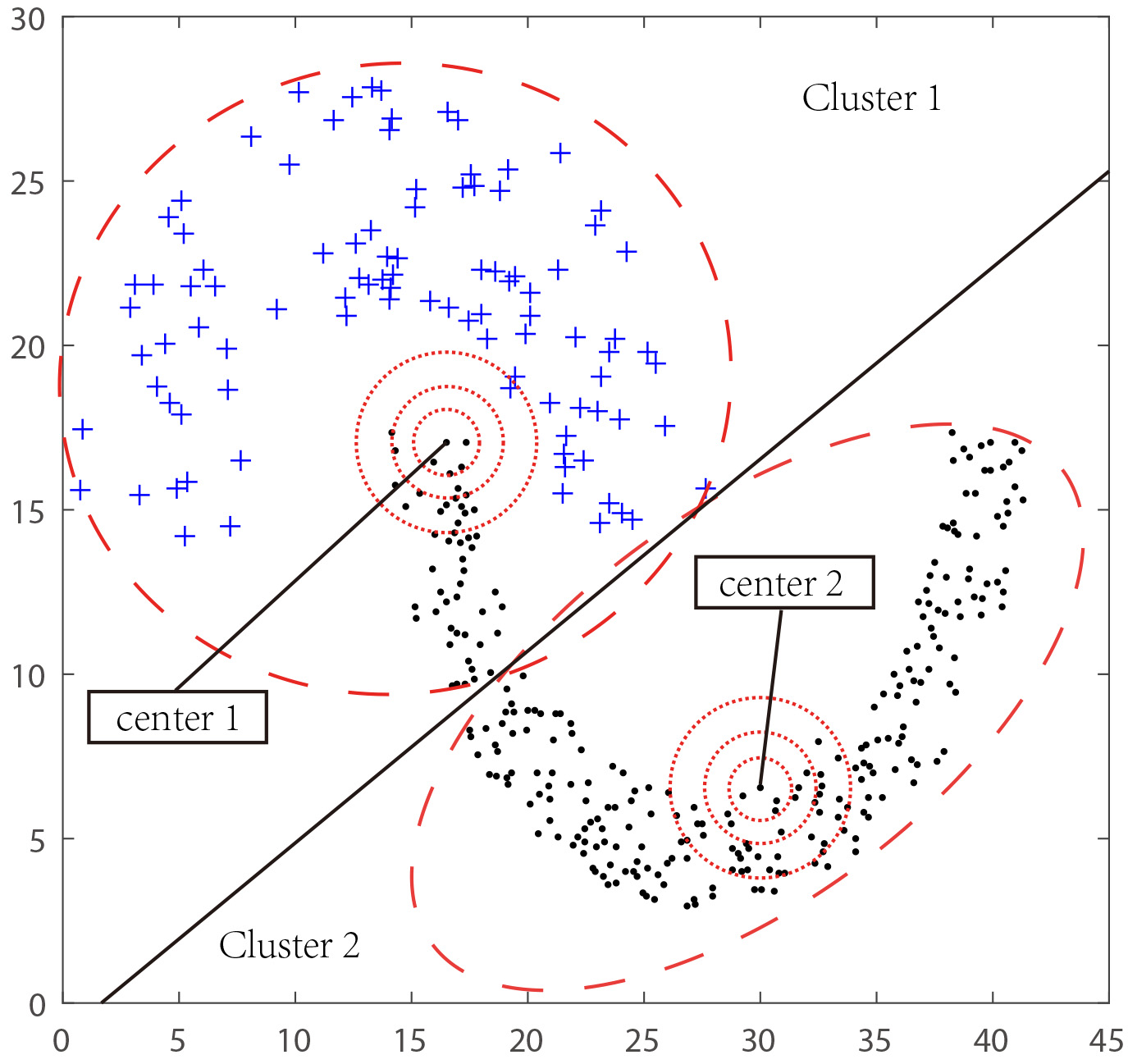
AGNES is a bottom-up hierarchical clustering method [20]. The following are three common inter-cluster distance calculation formulas:
where
According to Fig. 1, as the radius of the local space gradually shrinks, objects’ real classification in the local space becomes more consistent. Moreover, when such center-represented space shrinking, objects’ true labels become more reliable. Thus, assuming the label is accurate when the object described by the center of a cluster falls into the local space of the center. Define the space at a distance
where
Operation of MAGNES algorithm. (a) The base algorithm 1. (b) The base algorithm 2. (c) The base algorithm 3. (d) The base algorithm 4. (e) The base algorithm 5. (f) The base algorithm 6.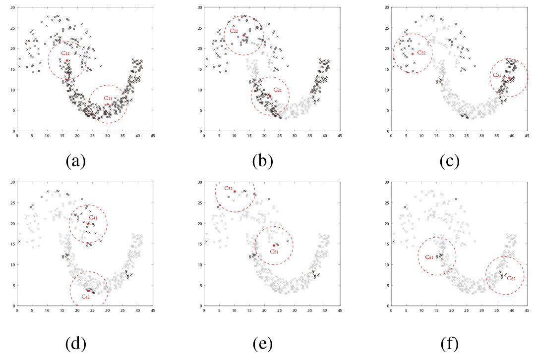
After addressing credibility issues, this part discusses how to generate multiple AGNES clusterings based on different local-credible spaces.
Since the points within the center neighborhood are already considered reliable, they are no need to participate in the next AGNES algorithm, which also ensures the local-credible spaces created by each algorithm are different from each other. Using
Such an iterative learning algorithm called the MAGNES algorithm is described as follows. Set
MAGNES: Multiple AGglomerative NESting algorithmDataset
Algorithm 2 shows the above iterative progress. The clustering process of the MAGNES algorithm is demonstrated on the dataset Jain [6]. Set
The MAGNES method has a
(a) Define the latent cluster (b) Exploring similarity through latent clusters’ density.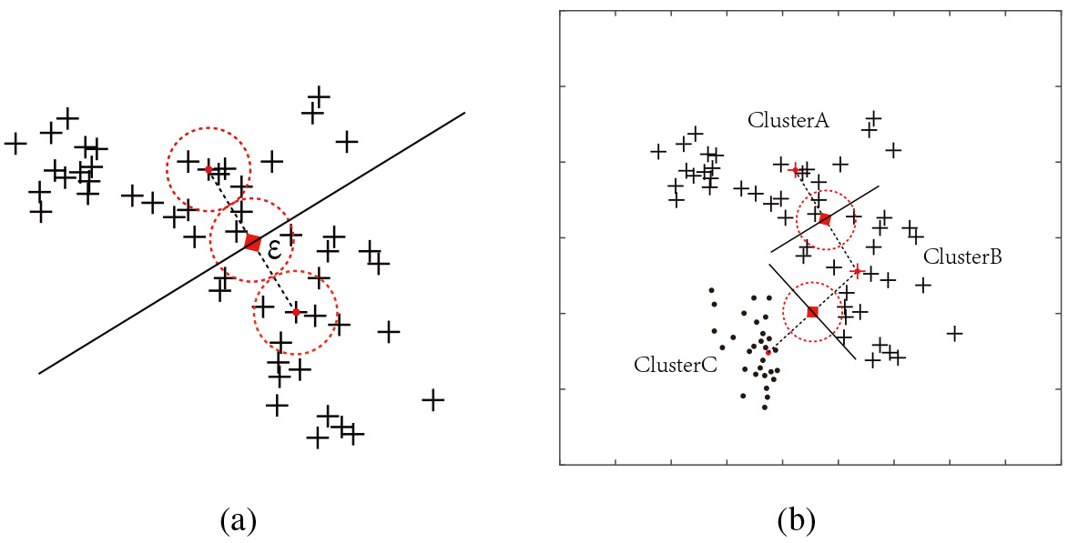
A classification label denotes a specific classification. However, a cluster label represents only the grouping attributes of the data, so different clustering results cannot be compared. Therefore, the labels of all clusterings need to be aligned. Moreover, when identifying non-convex datasets, the weakness of AGNES leads to the possibility that different clusters generated by a base clustering may represent the same true classification. Therefore, it is particularly important to analyze clusters’ relationships.
At this stage, there have been many measures to explore the similarity between clusters [33]. Among them, the algorithms constructed by Strehl [29] and Zhou [34] mentioned that the similarity can be judged using the number of objects common between different clusters, i.e., their overlap degree. Notably, such a measure cannot work when the two clusters share no items. To solve this dilemma and reasonably measure the degree of overlap, Iam-On [19] suggested a link-based measure. Although the above methods have given good ideas for calculating the inter-cluster similarity, none of them consider the effect of label credibility. In response to this, Bai et al. [4] have suggested a new similarity measure considering local-credible to overcome this drawback.
Considering local-credible spaces, they tried to measure two clusters’ similarity by computing the overlap between local-credible spaces.
Obviously, Fig.3a illustrates such a situation, the smaller
where
(a) Constructing the weight graph (b) Cutting the graph.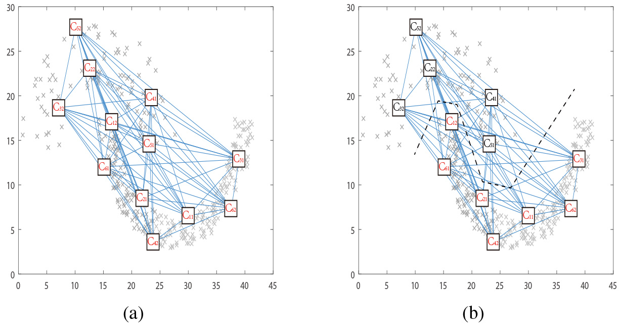
After achieving the similarity, building a graph that is undirected and weighted to capture inter-cluster relationships. The graph is denoted as
After getting the weighted graph, the construction of cluster relations can be viewed as a graph cut question with following objective function [28]:
The relation constructing procedure’s time complexity is
After fixing all cluster labels, for
The final clustering can be obtained by
The generation of the final clustering has a time complexity of
MAGNESCE: Multiple AGglomerative NESting Clustering ensemble AlgorithmDataset
Details of datasets: Amount of data (N), Data Dimension (D), Category Number (k)
Details of datasets: Amount of data (N), Data Dimension (D), Category Number (k)
The MAGNESCE algorithm is employed on above datasets and its effectiveness is evaluated by two clustering evaluation metrics. The experiments were conducted in the python programming environment. The hardware conditions are: OS: Windows enterprise ltsc(x64); processor: Intel(R) Core(TM) i5-8400 CPU @ 2.80 GHZ 2.81 GHZ; RAM: 16 GB.
Since the real datasets usually have missing values, the algorithm performance will be affected if the missing values cannot be handled effectively. For better comparison, five representative real data that have been processed well are selected in this section. The processing of missing values will be further discussed in the following paper. The datasets utilized are detailed in Table 1. Figure 5 depicts the images of the synthetic dataset, all datasets were obtained from [6, 1].
Evaluation criteria
Two common-used external criteria, adjusted rand index (ARI) [26] and normalized mutual information (NMI) [25], are used in this paper as similarity measures to assess the merits of clustering results. Assume a dataset
With values from Table 2, the ARI [26] is defined as
NMI [25] is calculated as
Similar table of the two classification
Similar table of the two classification
Images of the synthetic data. (a) Ring. (b) Atom. (c) T4.8k. (d) Chainlink. (e) Flame. (f) Complex. (g) Agg. (h) Jain.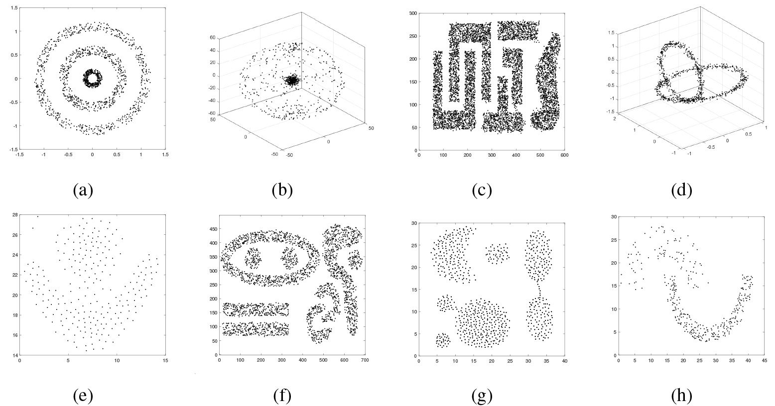
The more similar the clustering result and the true partition are, the higher the values of ARI and NMI will be.
To examine MAGNESCE, the following algorithms are used on fuzzy
The co-association similarity martix (CO) and the three link-based methods WCT, WTQ and CSM are the pairwise similarity method. To get the final solution, the average-link (AL) algorithms is used. Algorithms like CSPA, HGPA, MCLA proposed by Strehl and Ghosh are the graph-based methods. Feature-based methods contain the expectation maximization (EM) algorithm proposed by Topchy [30] and IVC algorithm proposed by Nguyen [24]. The multiple clustering algorithms FMKCE proposed by Bai [5].
Besides, to demonstrate the ability of MAGNESCE to identify non-convex divisions, three nonlinear algorithms still need to be taken into account: NSC (normalized spectral clustering algorithm) [23], DBSCAN (density-based spatial clustering of applications with noise) [12] and CFSFDP [27].
| Methods | Synthetic datasets | Real datasets | |||||||||||
|---|---|---|---|---|---|---|---|---|---|---|---|---|---|
| Ring | Atom | T4.8k | Chainlink | Flame | Complex | Agg | Jain | Digits | Wine | Statlog | Iris | Breast | |
| CO-AL | 0.1305 | 0.1456 | 0.5098 | 0.0927 | 0.4880 | 0.3726 | 0.6245 | 0.5853 | 0.6050 | 0.8471 | 0.5700 | 0.7302 | 0.7302 |
| WCT-AL | 0.1382 | 0.1456 | 0.4952 | 0.0927 | 0.4880 | 0.3635 | 0.7342 | 0.5853 | 0.6046 | 0.8471 | 0.5699 | 0.7302 | 0.7302 |
| WTQ-AL | 0.1389 | 0.1456 | 0.3326 | 0.0927 | 0.4880 | 0.3705 | 0.7081 | 0.5853 | 0.6049 | 0.8471 | 0.5699 | 0.7302 | 0.7302 |
| CSM-AL | 0.1448 | 0.1456 | 0.4956 | 0.0927 | 0.4880 | 0.4199 | 0.7192 | 0.5853 | 0.6146 | 0.8471 | 0.5699 | 0.7302 | 0.7302 |
| CSPA | 0.3163 | 0.0021 | 0.5010 | 0.0927 | 0.4312 | 0.3418 | 0.5365 | 0.2774 | 0.7573 | 0.7808 | 0.4329 | 0.6521 | 0.3414 |
| HGPA | 0.0004 | 0.0013 | 0.4012 | 0.0010 | 0.0038 | 0.1966 | 0.3621 | 0.0021 | 0.3750 | 0.1286 | 0.2619 | 0.1026 | 0.0007 |
| MCLA | 0.0004 | 0.1554 | 0.5018 | 0.0927 | 0.4880 | 0.3736 | 0.5778 | 0.5853 | 0.6935 | 0.8471 | 0.5127 | 0.7302 | 0.7302 |
| EM | 0.0302 | 0.2617 | 0.4775 | 0.0896 | 0.4164 | 0.3240 | 0.5682 | 0.5151 | 0.6205 | 0.7855 | 0.5074 | 0.6008 | 0.6328 |
| IVC | 0.3231 | 0.1178 | 0.4894 | 0.0927 | 0.3708 | 0.4097 | 0.5783 | 0.1288 | 0.6006 | 0.6875 | 0.4188 | 0.5970 | 0.0487 |
| NSC |
|
|
0.9260 |
|
0.8382 | 0.9848 | 0.9045 |
|
0.7536 |
|
0.5308 | 0.7455 | 0.7493 |
| DBSCAN |
|
0.3786 | 0.7780 | 0.4947 | 0.2270 | 0.8513 | 0.6294 | 0.2824 | 0.5052 | 0.3587 | 0.4319 | 0.5162 | 0.0478 |
| CFSFDP | 0.3227 | 0.4154 | 0.6098 | 0.6853 | 0.9337 | 0.8043 | 0.9898 | 0.6438 | 0.7584 | 0.7414 | 0.4963 | 0.7028 | 0.7305 |
| FKMCE |
|
|
0.9786 |
|
0.9539 | 0.9891 | 0.9909 |
|
0.8430 | 0.8834 |
|
0.8296 | 0.7700 |
| MAGNESCE |
|
|
|
|
|
|
|
|
|
0.8992 | 0.6115 |
|
|
NMI values of different methods
Before comparing, certain parameters should be set in advance, which are listed as follows:
Since MAGNESCE is based on the hierarchical clustering AGNES algorithm. Use the average-link to calculate the inter-cluster distance. Let the value of The DBSCAN, CFSFDP and FKMCE also need to find the right parameter For the NSC algorithm, using Gaussian kernel and its kernel parameter
The values of ARI and NMI of these algorithms are shown in Tables 4 and 4, respectively. Some of these data are from the [5, 4]. By bolding the highest value, it is easy to see that the MAGNESCE algorithm has superior accuracy to other algorithms on given datasets. The reason is that the fuzzy
According to Tables 4 and 4, the performance of ARI and NMI on real datasets is generally inferior to that on artificial datasets. This is since real datasets have a higher number of features than artificial datasets, leading to a strong sparsity of the similarity matrix
In addition, when
(a) Effect of parameter 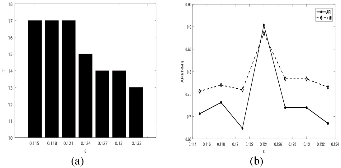
(a) Effect of parameter 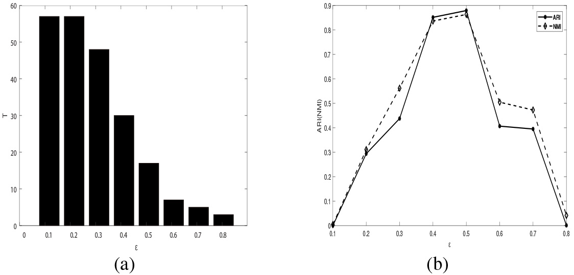
Noise points and missing values are the two main factors, which affecting the clustering performance. The effects of different treatments of noise points and missing values on the clustering results are discussed in this section.
Effect of noise points
This part takes the T4.8k dataset as an example for noise point discussion. Noise points are added to the T4.8k dataset, named T4.8k_noise. The clustering pictures of the algorithm on the original dataset and the noise dataset are shown in Fig. 8a and b. A comparison of the two datasets is shown in Table 5. Table 6 shows the ARI and NMI values of the MAGNESCE algorithm on the two datasets. Table 6 shows that the ARI and NMI values of the noise set are lower than those of the original dataset due to the presence of noise points.
From the above results, it is clear that noise points will affect the algorithm’s performance to some amount. As a consequence, while performing cluster analysis, pre-processed noise-free point data is typically employed to achieve the best results.
Comparison of original and noisy T4.8k dataset
Comparison of original and noisy T4.8k dataset
ARI and NMI for the original and noisy datasets
(a) No noise points (b) With noise points.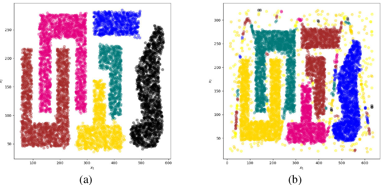
Description of the Dermatology dataset
Description of the Dermatology dataset
ARI and NMI obtained by different processing methods
Given that the real dataset contains a certain number of missing values under normal circumstances, this section will investigate the impact of various missing value processing methods on the algorithm’s performance. This section makes use of a dermatology dataset [1]. The detail of the dermatology dataset is in Table 7. Table 7’s final line displays the number of missing values (M). The data collection has 8 missing values. To handle these 8 missing values, two normal methods are used: the deletion method and the mean filling method. The deletion method deletes the data containing the missing value, whereas the mean filling method fills the missing value with the mean value of the column containing the missing value.
We used the above two methods on the dermatology dataset and obtained two new datasets, named Dermatology_delet and Dermatology_mean. Table 8 shows a comparison of the algorithm’s ARI and NMI on these two datasets. It shows that MAGNESCE has higher ARI and NMI values on the Dermatology_delet dataset than the values on the Dermatology_mean dataset. This is because the deletion method directly deletes the data with missing values without changing the original attributes of the data, whereas the mean filling method is very likely to cause a certain degree of deviation in the original data, and affects the algorithm’s clustering performance. As a result, when there are only a few missing values, the deletion method should be considered.
This paper proposes an ensemble framework called MAGNESCE to integrate AGNESs. The algorithm is divided into three main steps: constructing multiple AGNES algorithms, extracting label-credible objects in the local space of cluster centers, and producing the relation among clusters. This strategy improves the robustness and quality of AGNES so that arbitrarily shaped clusters can be well-identified. This paper also compares the MAGNESCE algorithm to other commonly used clustering algorithms and a multiple fuzzy k-means ensemble algorithm on several synthetic and real datasets. The experimental results show that the MAGNESCE algorithm is more effective than these algorithms. Furthermore, we hope to propose an efficient and general ensemble framework in the future, which does not require any more complex parameter adjustment operations.
Footnotes
Acknowledgments
The authors are very grateful to the editors and reviewers for their valuable comments and suggestions to improve the quality of this manuscript.