Dynamic gaussian deep belief network design and stock market application

Abstract

Stock price forecasting has been an important topic for investors, researchers, and analysts. In this paper, a prediction model of Dynamic Gaussian Deep Belief Network (DGDBN) is proposed. Generally, the network structure of traditional Deep Belief Network (DBN) determines the performance of its time series prediction. Most previous research uses artificial experience to adjust the network structure, it is difficult to ensure performance and time efficiency by constantly trying. In addition, the accuracy of the traditional DBN stacked by binary Restricted Boltzmann Machines(RBM) needs to be improved when solving the time series problem. The DGDBN designed in this paper contains two points: The first point is to add Gaussian noise to the RBM. The second point is to realize the increase or decrease branch algorithm of hidden layer structure according to the connection weights and average percentage error (MAPE). Finally, the forecast for the stocks of United Technologies Corporation and Unisys Corp, DGDBN is compared with DBN and LSTM. The root means square error (RMSE) increases by 15% and 65%. The interesting thing we found is that the number of neurons in the last layer of the DGDBN network has a greater effect than other layers.

Keywords

Deep belief network stock forecast dynamic network design continuous restricted Boltzmann machine

1. Introduction

Financial market data is non-linear, dynamic, complex, and chaotic, which is considered to be one of the most challenging problems in time series forecasting [1, 2]. Nevertheless, many empirical studies show that financial markets are predictable to some extent [3]. Scholars have tried to achieve relatively accurate predictions of financial markets, such as the Autoregressive Integrated Moving Average Model (ARIMA) [4] and Neural Network (NN) [5]. However, there are defects such as a large amount of calculation, easy to fall into a local minimum, and poor accuracy [6]. In recent years, deep learning has emerged as a particularly attractive candidate for financial forecast [7]. Deep Belief Network (DBN), as a core model of deep learning, has attracted much attention due to its real-time and good nonlinear capabilities [8]. It has played a role in a variety of machine learning problems, such as object recognition [9], image recognition [10], fault detection prediction [11], financial data prediction [12] et al.

DBN is a probabilistic generation model proposed by computer scientist and “Father of Neural Networks”, Geoffrey Hinton, which simulates the learning mechanism of the human brain for data feature processing [13]. As a deep network, DBN is stacked by Restricted Boltzmann Machine (RBM). The output of the previous RBM is the input of the next RBM [14]. In addition, DBN achieves the learning and extraction of data feature information through an unsupervised learning process [13]. Compared with the superficial network, it is better to learn from a large amount of data and find the underlying data rules. Through the previous research, we found that DBN still has some issues. First of all, the network structure is commonly a fixed structure set in advance, and the network structure does not change during the training process, which cannot guarantee the superiority of the initial network parameters. Secondly, when traditional DBN deals with continuous data, the prediction accuracy is reduced due to its discrete type. When DBN solves nonlinear data similar to stocks, different network structures will lead to reduced predictions or over-fitting [15]. The common methods for determining the network structure of neural networks include the empirical setting method [16], trial and error method [17], growth method, and pruning method. Basheer et al. designs the hidden neurons of artificial neural networks based on experience [15]. Zhao et al. proposed to delete hidden neurons in artificial neural networks based on weights [18].

Based on artificial neural network structure optimization, scholars began to examine how to construct an appropriate DBN network to better fit nonlinear data. However, compared with artificial neural networks, the research is still at the initial stage [19]. In the existing literature, most of the DBN network structures are designed through empirical methods and trial-and-error methods. Farahat M. et al. used the trial and error method to determine the structure of the DBN network and used it to noise-robust speech recognition [20]. Shen et al. set up the DBN network structure through manual experience used a conjugate gradient algorithm to accelerate learning and applied it to exchange rate prediction [21]. Regardless of the trial and error method or the manual experience method, it takes a lot of time, and it is difficult to guarantee that the result obtained is the optimal network structure. S.Pirmoradi et al. used the separability to automatically determine the network structure by using the average of the weights as the threshold, which improved the classification ability of the DBN single-layer network restricted Boltzmann machine [22]. Qiao et al. designed an organizational deep belief network based on the spike intensity and root mean square error of neurons, but this method has a large amount of calculation [23]. Zhang et al. designed a self-organizing DBN network, but only considered the hidden layer neurons, the hidden layer is fixed to two layers [24]. To solve the problem of DBN network structure, this article is based on the above research [18, 23]. Take the norm square root of the connection weights as the judgment basis to select the hidden layer neurons to discard or split, and then determine the depth of the neural network according to the average absolute percentage error of the network. This design method not only adjusts the number of hidden neurons but also considers the changes in the hidden layer. The resulting network retains the main structure of the original network, improves the network performance, and the calculation in the operation process is relatively simple.

As a component of DBN, RBM also affects the forecast effect of the DBN model. Although the traditional DBN has achieved good results in the field of artificial intelligence, the accuracy of time series prediction still needs to be improved. The traditional DBN network uses a discrete method in feature extraction, which is essentially due to the traditional DBN network is composed of binary restricted Boltzmann machine stack (RBM), so the effect of processing continuous data is poor [25]. To solve this problem, some scholars have proposed a continuous RBM network. Zhang converts discrete input layer signals of restricted Boltzmann machine (RBM) into continuous signals by adding Gaussian noise, converts discrete RBM into continuous RBM, and makes exchange rate prediction with the proposed model [26]. However, this method only considers the RBM of the input layer. In this paper, by adding Gaussian noise to RBM and combining it with the structural change of the DBN network, we increase the RBM with Gaussian noise layer by layer. Compared with previous studies, the method proposed in this paper ensures that each layer of the unit network is a continuous restricted Boltzmann machine, which improves the prediction performance of traditional DBN for continuous data.

Based on the above discussion, a dynamic Gauss Depth Belief Network (DGDBN) is proposed, which optimizes the performance of traditional DBN in time series prediction and has three main contributions:

•
To improve the prediction effect of traditional DBN in time series prediction, Gaussian noise is added to the restricted Boltzmann machine so that continuous data can be better processed.
•
It is proposed for the first time to determine the number of hidden layer neurons and hidden layer according to the root of the quadratic norm and the average absolute percentage error of connection weights between layers, so as to dynamically adjust the DBN network structure in the training process.
•
The relationship between the prediction performance of DGDBN during training and the number of network structure layers and neurons is analyzed and summarized.

The rest of the paper is organized as follows. Section 2 briefly introduces theoretical knowledge. In Section 3, the detail of DGDBN model is proposed. The stock market experimental validation and analysis of DGDBN is performed in Section 4. Finally, Section 5 concludes our findings and presents a number of directions for future study.
2. Related work

2.1 Gaussian deep belief network

Deep Belief Network (DBN) is a probability generation model stacked by the Restricted Boltzmann machine (RBM). RBM is a single-layer neural network with randomness, which is essentially an undirected graph model composed of a random layer of visible neurons (input layer) and a layer of hidden neurons [27]. The RBM model is fully connected between layers, but there is no connection within layers. Figure 1 shows the model diagram of RBM. V represents the visible layer, H represents the hidden layer, and W represents the connection weights between the visible layer and the hidden layer.

Figure 1.

The structure of RBM model.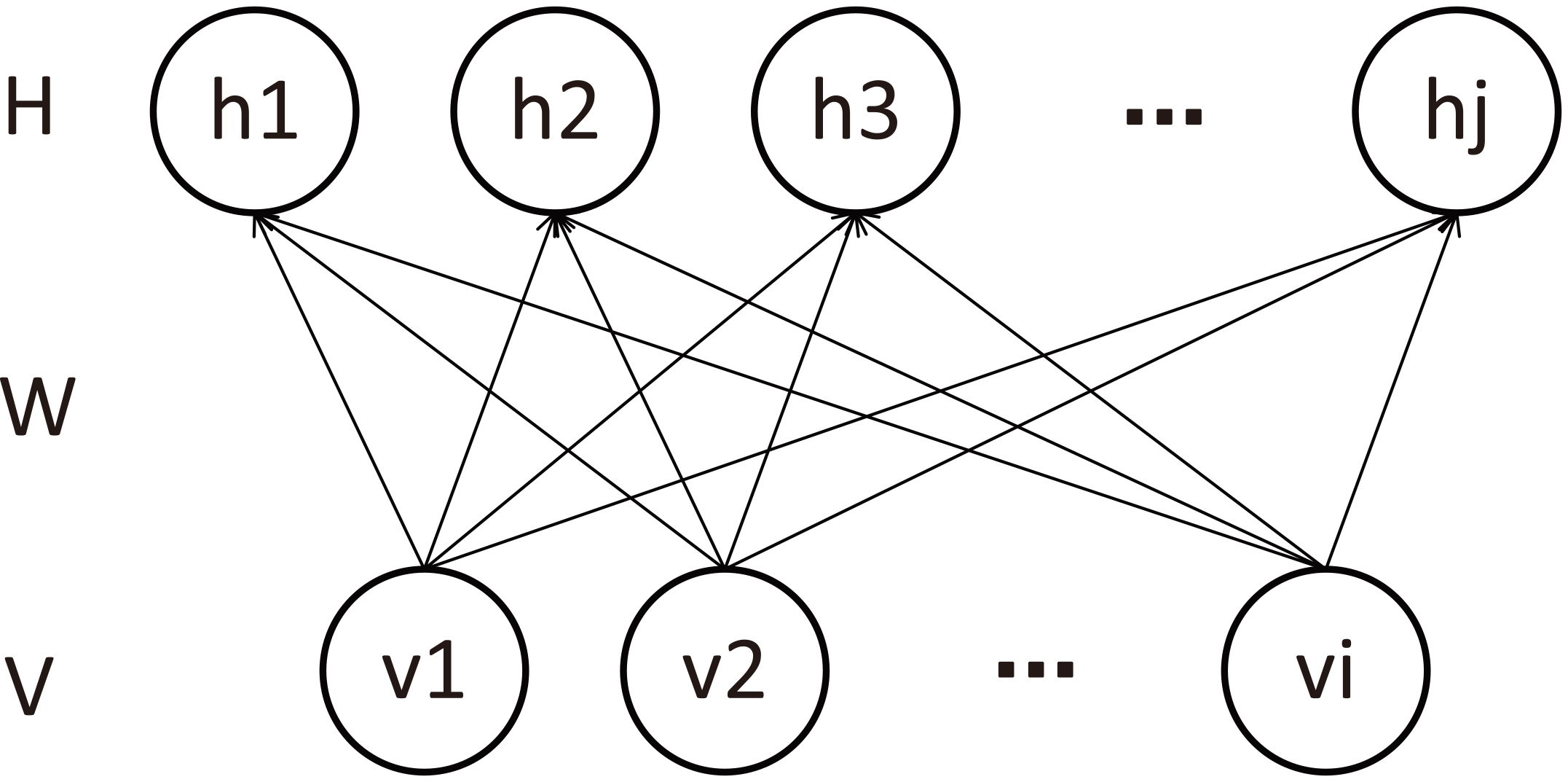

RBM as a model based on energy function, the energy function $E(v,h)$ between the visual layer vector V and the hidden layer H of RBM is:

$\displaystyle E(v,h)=-\sum_{i=1}^{nv}\sum_{j=1}^{nh}v_{i}h_{j}w_{ij}-\sum_{i=1% }^{nv}v_{i}b_{i}-\sum_{j=1}^{nh}h_{j}a_{j}$ (1)

where $v_{i}$ is the $i$ node of the visible layer node, $h_{j}$ is the $j$ node of the hidden layer node, $w_{i}^{j}$ is the connection weights between the visible node $i$ and the hidden node $j$ , $a$ and $b$ are the offset of the visible layer and the hidden layer, $n v$ and $n h$ represent the number of nodes of the visible layer and the hidden layer.

From Eq. (1), it can be deduced that the joint function between visual layer V and hidden layer H is:

$\displaystyle{p}\left(v,h\right)=\frac{{{\exp}^{-E\left(v,h\right)}}}{Z}$ (2)

where $Z$ is the normalization factor, and its calculation formula is:

$\displaystyle Z\text{=}\sum\limits_{\text{nv,nh}}{{{e}^{-E\left(v,h\right)}}}$ (3)

Because there is no link between neurons in the same layer of RBM, it can be concluded that the conditional probability of visible layer neurons and hidden layer neurons is:

$\displaystyle{p}\left(h_{j}=1|v\right)=\textit{sig}\left(\sum\limits_{i=1}^{nv% }{{{v}_{i}}{{w}_{ij}}}+{{b}_{j}}\right)$ (4) $\displaystyle{p}\left(v_{i}=1|h\right)=\textit{sig}\left(\sum\limits_{j=1}^{nh% }{{{h}_{j}}{{w}_{ji}}}+{{a}_{i}}\right)$ (5)

where $p\left(h_{j}=1\middle|v\right)$ represents the activation probability of the j hidden neuron, $p\left(v_{i}=1\middle|h\right)$ represents the activation probability of the $i$ input neuron, $s i g$ is the Sigmoid function, its formula is defined as:

$\displaystyle\textit{sigmoid}\left(\text{x}\right)=\frac{1}{1+{{e}^{-x}}}$ (6)

Traditional DBN may map continuous data into discontinuous binary data according to Eqs (4) and (5). Therefore, this paper adds Gaussian noise on this basis to ensure the continuity of RBM in the training process. After the change, the conditional probability of the visible layer neuron and the hidden layer neuron is:

$\displaystyle{p}\left(h_{j}=1|v\right)=\textit{sig}\left(\sum\limits_{i=1}^{nv% }{{{v}_{i}}{{w}_{ij}}}+{{b}_{j}}\text{+}N(0,1)\right)$ (7) $\displaystyle{p}\left(v_{i}=1|h\right)=\textit{sig}\left(\sum\limits_{j=1}^{nh% }{{{h}_{j}}{{w}_{ji}}}+{{a}_{i}}\text{+}N(0,1)\right)$ (8)

where $N(0,1)$ represents a Gaussian variable with mean of 0 and variance of 1.

2.2 Model training process

The training process of the Gaussian deep belief network is the same as the traditional deep belief network. Its training process is divided into two steps: unsupervised training and supervised training, as shown in Fig. 2 Unsupervised training is to train RBM layer by layer to ensure that each layer of RBM reaches the optimal state at the end of training. This process is a greedy algorithm and can not ensure that the overall structure reaches the optimal state. After unsupervised training, the parameters of each layer are adjusted reversely layer by layer according to the error between the output of the last layer RBM and the real value. This process also solves the problem caused by a greedy algorithm in the process of unsupervised training.

Figure 2.

The structure of GDBN model.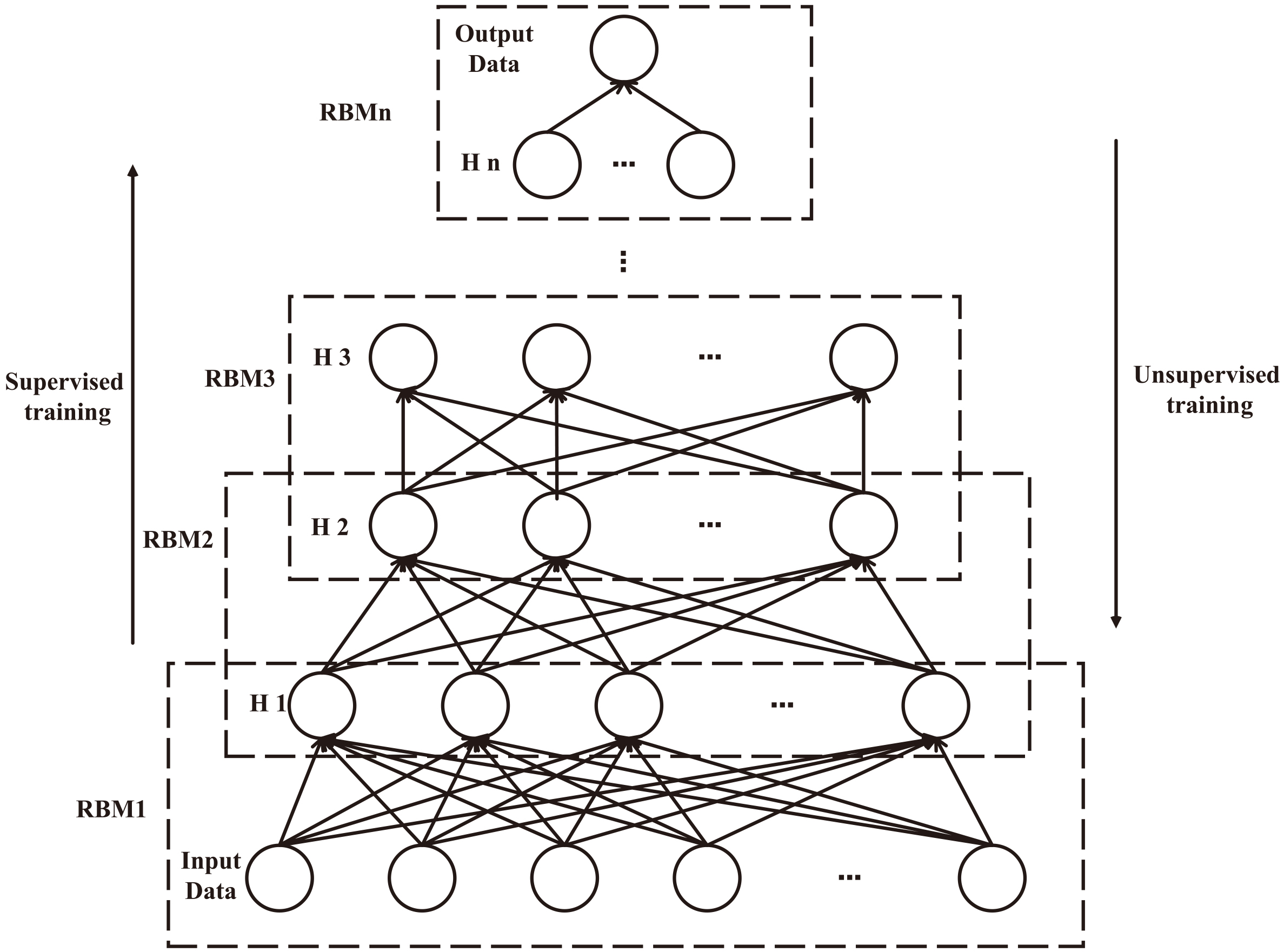

In the unsupervised training process, the training goal of RBM is to maximize the fitting of the input data by calculating the maximum likelihood estimation of the input data to make Eq. (2) maximum. In the solution process, the conditional probability is calculated alternately through Eqs (7) and (8) to maximize the final reconstruction error. This process is called Gibbs sampling, as shown in Fig. 3. However, too many iterations in Gibbs sampling lead to a long calculation time [28]. In this paper, the Contrastive Divergence (CD) algorithm is used to train RBM. Taking $k=$ 1, that is, the Gibbs sampling process is only iterative once.

After the unsupervised training, the model enters the supervised training. In this process, we use the classical BP algorithm to reverse fine-tune the parameters of DBN.

Figure 3.

Gibbs sampling process.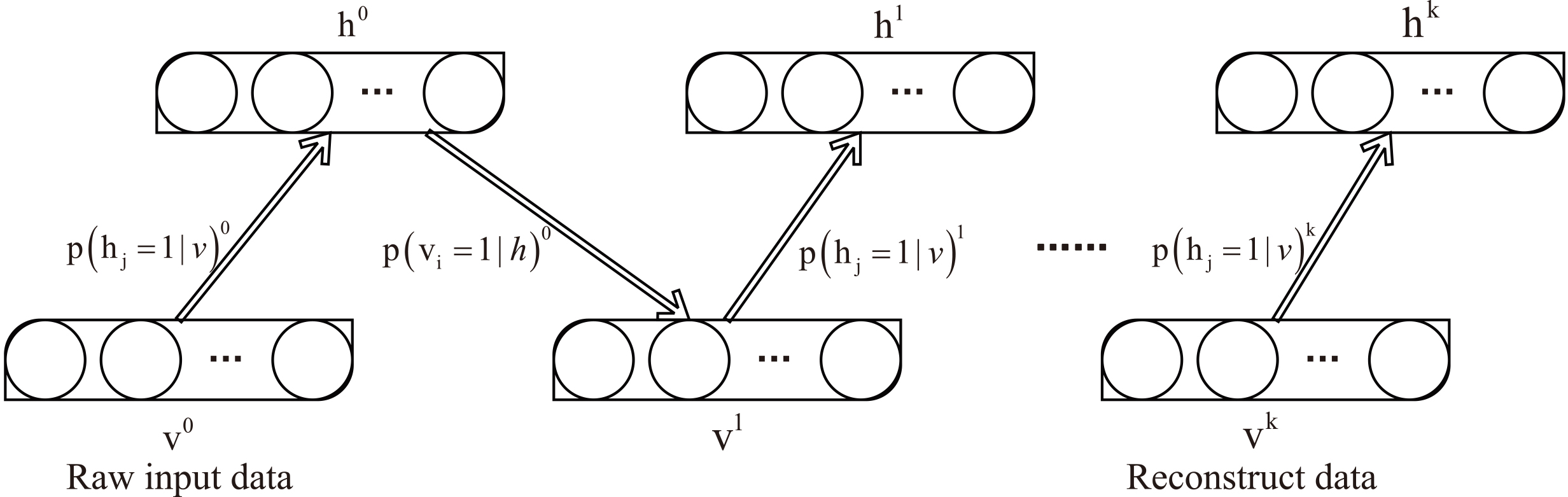

In fact, GDBN training is the process of mapping the visual layer data to the hidden layer. In an ideal state, although the data form changes the hidden layer data contains the same information as the visual layer. As shown in Fig. 2, we need to evaluate how many hidden neurons and hidden layers can ensure that the hidden layer data is infinitely close to the visual layer. Artificial experience testing requires a lot of energy and time, so we designed a Dynamic Gaussian Deep Belief Network (DGDBN), which not only ensures that Gaussian noise is added to each layer of the network but also can automatically find the optimal network structure.

3. Design of DGDBN model

In this section, we present the main ideas of the DGDBN model. Report to the fixed network structure of traditional DBN. DGDBN has two areas of improvement: segmentation or deletion of hidden layer neurons; adding Gaussian RBM hidden layer. The method used in the two improvements and the training process of the DGDBN model is described as follows:

3.1 Split and delete hidden layer neurons algorithm

After trial and error on the single-layer GDBN model. We discovered that when the number of neurons is too small, the information contained in the neurons in the visual layer will be lost during the mapping process. Upper layer neurons cannot capture complete feature information. Therefore, the prediction effect of the network will be lowered. When there are too many hidden neurons, redundant data information will be mixed, resulting in overfitting of the network model. In short, too many or too few hidden layer neurons will lead to a decrease in the prediction effect of the model network.

In order to select an appropriate number of hidden neurons, it is necessary to add or delete hidden neurons. The change of the number of neurons will affect the change of the connection weights. In this paper, the increase or decrease of the hidden neurons depends on the quadratic norm square root $N_{i}$ , which is calculated by the following formula.

$\displaystyle N_{i}=\sqrt{\sum\limits_{j=1}^{n}w_{ij}^{2}}$ (9)

$N_{i}$ is the quadratic norm root of neurons i in the visual layer after the training of the single-layer restricted Boltzmann machine. $w_{ij}$ is the connection weights between visual layer neurons i and hidden layer neurons $j$ . n is the number of hidden layer neurons. According to Eqs (7)–(9), it can be seen that when the value of $i$ is too small, the output of neuron $j$ is also small after the activation function Sigmoid. This shows that neuron $i$ has little effect on the output of the next layer. It can be deleted, on the contrary, the neuron is retained and divided.

For deleting or splitting hidden neurons, the following criteria are designed according to the principle of multiple stepwise regression.

First, calculate the sum of $N_{i}$ and find a single $N_{i}$ relative proportion $R_{i}$ , the calculation process is:

$\displaystyle R_{i}=\frac{N_{i}}{\sum\limits_{i=1}^{n}N_{i}}$ (10)

Then, $R_{i}$ sorted from large to small, and calculated the cumulative value MR.

Finally, the thresholds $\textit{MR}_{0}$ and $\textit{MR}_{1}$ of the accumulated value MR are set. When MR is less than $\textit{MR}_{0}$ , the accumulated hidden neurons are split. When MR is greater than $\textit{MR}_{0}$ and less than $\textit{MR}_{1}$ , the accumulated neurons are retained. When MR is greater than $\textit{MR}_{1}$ , the neurons that are not accumulated are discarded. According to experience and trial and error, $\textit{MR}_{0}$ is set to 0.05, that is, the neurons with the output ratio of the top 5% are divided. $\textit{MR}_{1}$ is set to 0.85, the first 85% of neurons can map the main information of the data, and neurons with a smaller output can be discarded.

The network obtained by the above method not only deletes redundant neurons, but also splits a small number of important neurons. Ultimately, the structure of the DBN network is optimized and the prediction accuracy of the network is improved.

3.2 Add and delete Gaussian RBM hidden layer algorithm

When the DBN of a single hidden layer has enough neurons, it can approximate most nonlinear systems [29]. But it cannot well fit high complexity and nonlinear systems. The single-layer DBN needs to increase the hidden layer and hidden neurons to improve the nonlinear fitting rate. Taking into account the network prediction error rate changes, the addition and deletion of hidden layers are judged according to the average absolute percentage error (MAPE) of the prediction results.

During the network training process, we set the MAPE threshold $\textit{MAPE}_{0}$ . In this paper, $\textit{MAPE}_{0}$ is set to the MAPE we expect the model results to achieve. A hidden layer is added when the actual MAPE satisfies the Eq. (11) condition. When the actual MAPE satisfies Eq. (12) and does not satisfy Eq. (11) , it means that the prediction effect of the network has declined, and the last hidden layer added should be deleted.

$\displaystyle\textit{MAPE}\geqslant\textit{MAP}E_{0}$ (11) $\displaystyle\textit{MAP}E_{r}>\textit{MAP}E_{r-1}$ (12)

where $\textit{MAPE}_{r}$ in Eq. (12) represents the average percentage error rate of a network with $r$ hidden layers, when it is greater than the percentage error rate of a network with $r-1$ hidden layers, the newly added hidden layers are deleted.

3.3 DGDBN training process

Figure 4.

DGDBN training flowchart.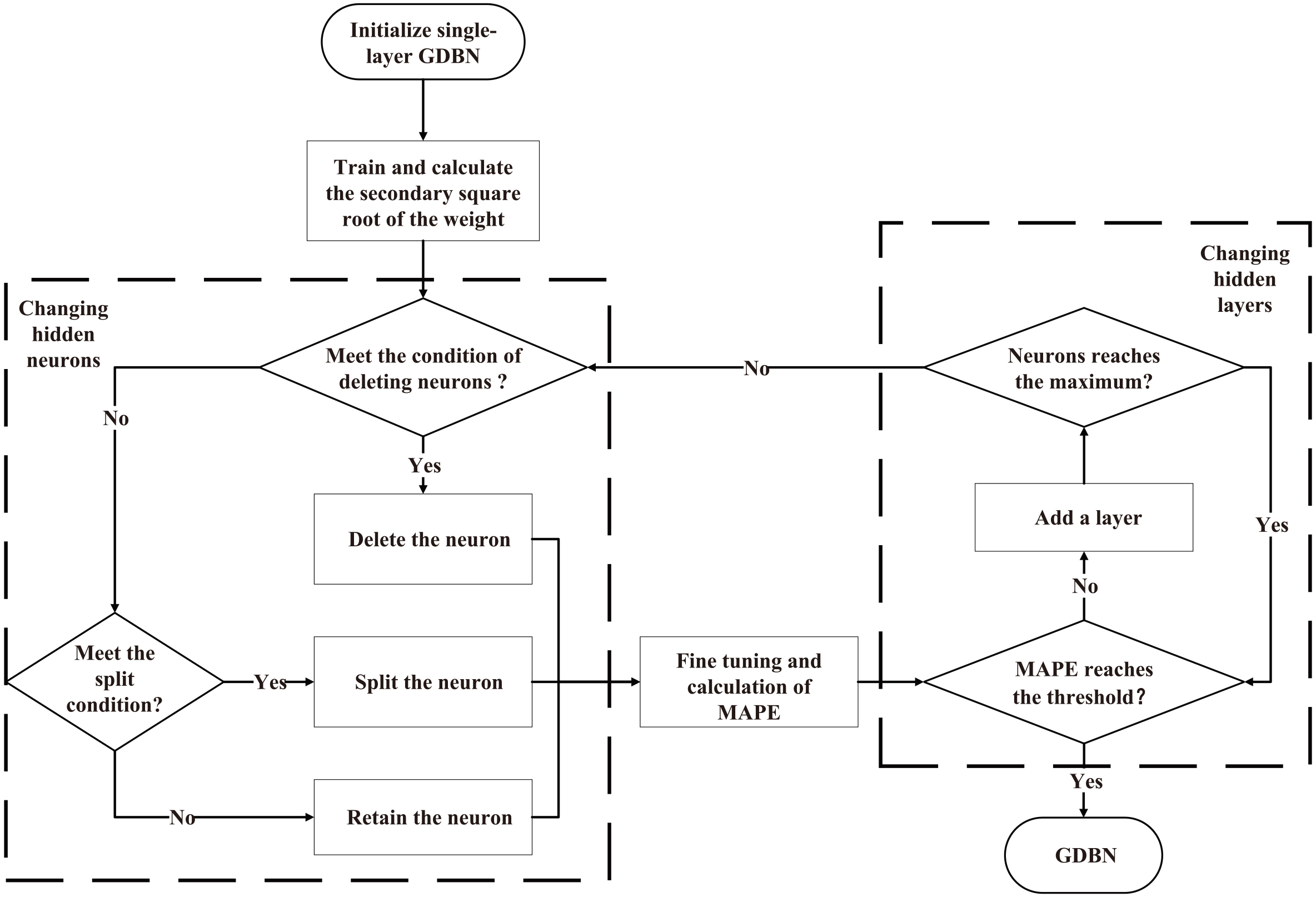

Based on the GDBN training introduced in Section 2.2, the DGDBN model dynamically adjusts the network structure according to the methods introduced in Sections 3.1 and 3.2. The training flowchart is shown in Fig. 4. The specific steps are described as follows:

Step 1:

Initialize a single-layer Gaussian RBM, the number of neurons in the hidden layer can be given arbitrarily. After Gibbs sampling, RBM splits and deletes neurons according to the method of Section 3.1.

Step 2:

Calculate the MAPE of the network at this time, and add a new Gaussian RBM if Eq. (11) is satisfied. The number of neurons in the hidden layer ranges from half to equal to the number of neurons in the upper layer.

Step 3:

Repeat steps (1) and (2) until the MAPE of the network satisfies Eq. (11) or the MAPE of the network begins to increase. The network training is terminated.

The main algorithms in the training process are given in Algorithm 4, which mainly include the training function of each layer of RBM and the increase of the hidden layer function.

The training process of DGDBN[1] train set: $X_{\textit{train}}$ ; test set: $X_{\textit{test}}$ ; number of hidden units: $h_{n}$ ; learning rate: $\eta$ ; number of train epoch: $e_{t}$ ; number of finetune epoch: $e_{f}$ ; connecting weights: $W$ ; the bias: $h_{\textit{bias}},v_{\textit{bias}}$ weights matrix: $W$ ; the bias: $h_{\textit{bias}},v_{\textit{bias}}$ ; number of hidden units: $h_{n}$ $\textit{Initializing DBN with one layer and}W,h_{\textit{bias}},v_{\textit{% bias}}$ TRAIN_DBN $X_{\textit{train}},h_{n},W,e_{t}$ $//$ training RBM by CD algorithm $i=0,i<e_{t},i++$ Update the weights and bias of DBN Calculate $N_{i}$ according to W using Eq. (9) Calculate $R_{i}$ using Eq. (10) $\textit{sum}(R_{i})<\textit{MR}_{0}$ The accumulated neurons split into two neurons and copy the weights $\textit{sum}(R_{i})<\textit{MR}_{1}$ Delete unused neurons FINETUNE_DBN $X_{\textit{train}},h_{n},W,e_{f}$ $i=0,i<e_{f},i++$ Calculate $E$ using Eq. (1) Adjust $W,h_{\textit{bias}},v_{\textit{bias}}$ accoding to $E$ DBN_PREDICT $X_{\textit{test}}$ Predict the value $y_{\textit{predict}}$ according to DBN Calculat MAPE based on the real value $y_{\textit{real}}$ and predicted value $y_{\textit{predict}}$ $\textit{MAPE},y_{\textit{predict}}$ $\textit{MAPE}>\textit{MAPE}_{0}$ DBN_ADDLAYER $h_{n}$ $i=h_{n}[-1]/2,i<h_{n}[-1],i=i+10$ Executive function TRAIN_DBN Executive function FINETUNE_DBN Executive function DBN_PREDICT MAPE is greater than last resultcontinue $\textit{DBN},H_{n},\textit{MAPE},y_{\textit{predict}},h_{\textit{bias}},v_{% \textit{bias}}$

4. Simulation studies

In this section, two groups of different stock data were used to demonstrate the effectiveness and superiority of the proposed DGDBN. Moreover, the results were compared with DBN and LSTM. To reduce the influence of other irrelevant factors on the simulation results, the compilation software and operating environment of all simulation experiments are set as follows: the compilation software is PyCharm 2020.1 version, the operating environment is Microsoft Windows 10, the computer clock frequency is 2.1 GHz, and the RBM is 12.0 GB. Four benchmark evaluation functions are used to evaluate the performance of the model: root means square error $(\textit{RMSE})$ , R-square $(R^{2})$ , mean absolute percentage error $(\textit{MAPE})$ , mean absolute error $(\textit{MAE})$ .

$\displaystyle\textit{RMSE}=\sqrt{\frac{\sum_{i=1}^{n}{(y_{i}-\hat{y}_{i})}^{2}% }{n}}$ (13) $\displaystyle R^{2}=1-\frac{\sum_{i=1}^{n}{(y_{i}-\hat{y}_{i})}^{2}}{\sum_{i=1% }^{n}{(y_{i}-\bar{y})}^{2}}$ (14) $\displaystyle\textit{MAE}=\frac{\sum_{i=1}^{n}|y_{i}-\hat{y}_{i}|}{n}$ (15) $\displaystyle\textit{MAPE}=\frac{1}{n}\sum_{i=1}^{n}\frac{|y_{i}-\hat{y}_{i}|}% {y_{i}}$ (16)

where $n$ is the number of sample data. $y_{i}$ , ${\hat{y}}_{i}$ is the target output value and the actual output value of the $i$ sample.

4.1 Stock closing price (SCP) prediction

The SCP is one of the most concerning indicators in the stock financial market. Therefore, it is necessary to accurately predict the future closing price of stocks. In this paper, a model-based method is used to predict the closing price of the two sets of stock data using the proposed DGDBN.

4.1.1 Data

We used two sets of stock data in the experiment. Tables 1 and 2 respectively show part of the information of the two sets of data.

The first one is the stock data of United Technologies Corporation (UTX) from September 4, 2012, to September 1, 2017. The data comes from Yahoo Finance (https://finance.yahoo.com/). It contains 1258 pieces of data, of which 1004 pieces of data are used as training data, and the remaining 250 pieces of data are used as test data.

The second group is Unisys Corp (UIS) stock data from October 1, 2008, to November 10, 2017. The data comes from the New York Stock Exchange (https://www.nyse.com/index). There are 2296 pieces of data, 1833 pieces of data are used as training data, and 459 pieces of data are used as test data.

Table 1
Some historical data of UTX stock

Date	Opening price	Highest price	Lower price	Adjusted closing price	Volume
2013/4/1	93.16	93.41	92.70	83.66335	2543400
2013/4/2	93.15	93.54	92.85	83.72638	2586400
2013/4/3	93.15	93.97	93.01	83.91547	4407400
2013/4/4	93.37	93.80	92.96	83.87945	3029500
2013/4/5	92	92.75	91.90	83.41126	2564800
2013/4/8	92.84	93.72	92.42	84.37466	2386000
2013/4/9	93.94	94.58	93.38	85.04096	3181300
2013/4/10	94.72	95.70	94.64	85.69823	3780200
2013/4/11	95.52	95.84	95.17	86.27448	3908900
2013/4/12	95.63	95.69	95.17	86.15743	2539600
2013/4/15	95.37	95.48	93.50	84.20359	3956200
2013/4/16	94.40	94.82	93.72	85.09496	2843400

Table 2

Some historical data of UIS stock

Date	Open	High	Low	Volume	Close
2014/1/2	33.40	33.45	32.57	518834	32.97
2014/1/3	32.89	33.11	32.23	560422	32.98
2014/1/6	33.24	33.95	33.18	628581	33.45
2014/1/7	33.62	33.73	33.25	464832	33.63
2014/1/8	33.66	33.90	33.34	355586	33.55
2014/1/9	33.63	34.14	33.50	522893	33.74
2014/1/10	33.03	33.12	31.58	1295440	31.74
2014/1/13	31.69	32.32	30.76	773074	31.12
2014/1/14	31.25	32.81	31.25	532075	32.79
2014/1/15	32.83	33.47	32.63	636837	33.12
2014/1/16	32.97	33.19	32.72	352843	32.96
2014/1/17	32.88	33.10	32.36	387666	32.53

In order to prevent the influence of abnormal data on the prediction results, we use box plots to filter out abnormal data in the two groups of data. The judgment results of the box plot are shown in the Fig. 5.

Figure 5.

Box plot judgment results.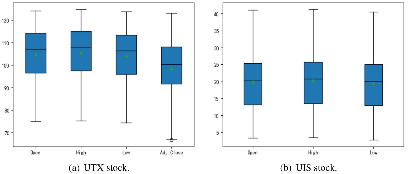

Replace abnormal data according to the following formula.

$\displaystyle x_{i}=\frac{x_{i-1}+x_{i+1}}{2}$ (17)

Where $x_{i}$ represents the abnormal data of the $i$ th day, $x_{i-1}$ represents the data of the previous day, and $x_{i+1}$ represents the data of the next day. That is, the abnormal data is replaced by the average value of the data of the previous and previous days.

All the sample data are standardized by Min-Max normalization. For each value of the sample data, the normalization calculation formula is:

$\displaystyle X_{\textit{norm}}^{i}=\frac{x_{i}-x_{\min}}{x_{\max}-x_{\min}}$ (18)

Where $x_{\textit{norm}}^{i}$ represents the normalized value of the sample data $x_{i}$ , $x_{\textit{min}}$ and $x_{\textit{max}}$ are the minimum and maximum values in the sample data set.

4.1.2 Experimental design and result

For the closing price prediction of the two groups of data, the time sliding window takes five, that is, the closing price on the fifth day is predicted by using the data information of the past four days. At the beginning of the simulation experiment, the initial network structure is a single-layer Gaussian depth belief network, and the number of iterations is 600 in the unsupervised training process; In the process of supervised training, the number of iterations is 300. Preset $\textit{MAPE}_{0}=$ 0.0055, $\textit{MR}_{0}=$ 0.05, $\textit{MR}_{1}=$ 0.85. During the experiment, after the training of the single-layer restricted Boltzmann machine, the neuron addition process is completed through the algorithm introduced in Section 3.1. After the network fine-tuning, if the MAPE does not reach the threshold, increase the initial number of neurons in the hidden layer, and test from 1/2 of the number of neurons in the upper hidden layer until it is equal to the number of neurons in the upper hidden layer, or MAPE shows an increasing trend; If MAPE reaches the threshold, network training ends.

The model structure of DGDBN gradually tends to be stable in the training process. In the first group of experiments, the hidden layer neurons initializing the single-layer Gaussian depth belief network are 100, and the final stable structure is 81-59-49. That is, the number of hidden layer neurons is $h_{1}=$ 81, $h_{2}=$ 59, and $h_{3}=$ 49. The prediction results of the experiment are shown in Fig. 6. In the second group, the number of hidden layer neurons initializing the single-layer Gaussian depth belief network is 50, and the final stable structure is 40-34-22-18. That is, the number of hidden layer neurons is $h_{1}=$ 40, $h_{2}=$ 34, $h_{3}=$ 22, and $h_{4}=$ 18. The prediction results of the experiment are shown in Fig. 6.

Figure 6.

DGDBN forecast results.

During the experiment, we recorded the MAPE value of the network prediction result after each change in the number of hidden layer neurons and hidden layers, as shown in Fig. 7. Through the study of the changing trend of MAPE in two groups of experiments, we found that the value of MAPE will increase when adding a new hidden layer. This is because when adding a new hidden layer in the experimental process, the number of neurons is 1/2 of the number of neurons in the upper hidden layer. At this time, there are too few neurons in the last hidden layer, which reduces the prediction performance of the model. With the increase of the number of hidden neurons in this layer, neurons can map more data information, MAPE decreases gradually, and finally reaches a stable state. This shows that for the DGDBN network, the number of neurons in the last layer has a greater impact on the network effect.

Figure 7.

The value of MAPE in network structure changes.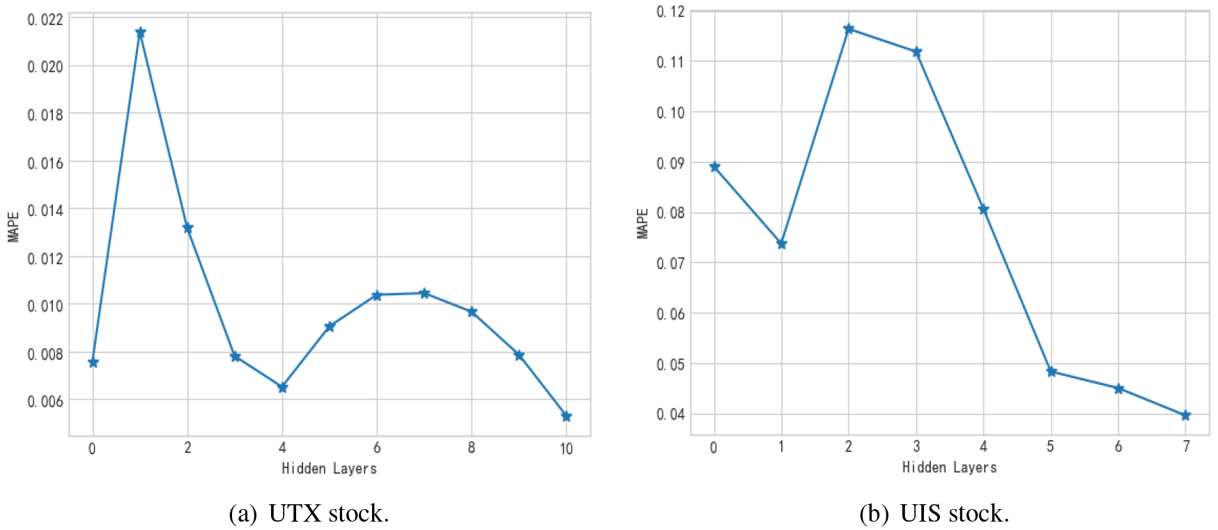

4.2 Model comparison and discussion

The main purpose of this study is to evaluate the performance of DGDBN in stock forecasting. In this section, the DGDBN model proposed in this paper is compared with the traditional DBN and LSTM. For the traditional DBN model, the network structure is set to the same number of hidden layer and hidden layer neurons before the dynamic change of the network. As for the activation function, DGDBN and DBN adopt the same Sigmoid activation function, LSTM takes its better activation function Relu. In order to reduce the influence of other parameters on the experimental comparison results, the training times are 300, and 128 sample data are processed each time. The comparison results of DGDBN, DBN, and LSTM are shown in Fig. 8.

Figure 8.

Comparison of DDBN, LSTM and DBN.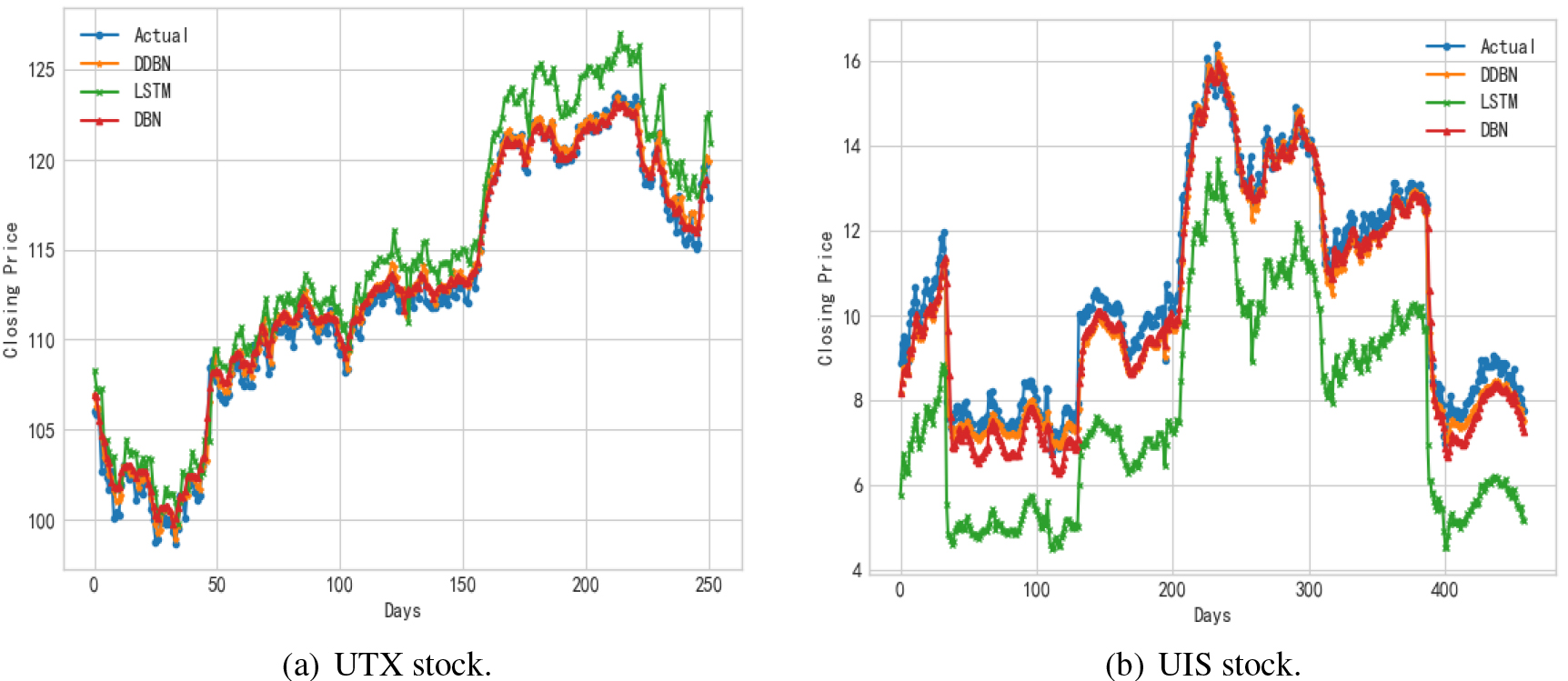

Figure 9.

Comparison of evaluation indexes (UTX stock).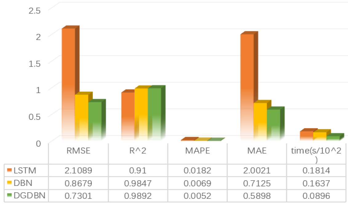

It can be seen from Fig. 8 that the DGDBN model proposed in this paper has a better fitting effect. For the test set of UTX, the MAPE of DBN is 0.0064, that of LSTM is 0.0175, and that of DGDBN is 0.0052. For the test set of UIS, the MAPE of DBN is 0.0505, that of LSTM is 0.2794, and that of DGDBN is 0.0396. Therefore, it can be seen that the prediction effect of the DGDBN model on stock closing price is better than DBN and LSTM. Although the prediction effect of DBN is better than LSTM, it is obvious that the prediction effect of the DGDBN model after network dynamic adjustment is better. DGDBN can better capture data information and determine the appropriate network structure by adding hidden layers and hidden neurons while deleting DBN redundant neurons.

Figure 10.

Comparison of evaluation indexes (UIS stock).

After 20 independent experiments, the following table shows the average results predicted by DGDBN, DBN, and LSTM models. Figure 9 shows the experimental results of UTX data, and Fig. 10 shows the experimental results of UIS data. In UTX data, the RMSE of LSTM is 2.1089, the RMSE of DBN is 0.8679, and the RMSE of DGDBN is 0.7301, which is 65% and 15% higher than that of LSTM and DBN respectively. In UIS data, the RMSE of LSTM is 2.8349, the RMSE of DBN is 0.5685, and the RMSE of the DGDBN is 0.4812, which is 83% and 15.4% higher than that of LSTM and DBN respectively. It can be seen from Figs 9 and 10 that the overall accuracy of DGDBN model is higher. In addition, the prediction time of the DGDBN model is slightly improved compared to DBN and LSTM. In UXT stock, the prediction time of LSTM is 18.14, the prediction time of DBN is 16.37, the prediction time of DGDBN is 8.96; In UIS stock, the prediction time of LSTM is 24.85, the prediction time of DBN is 10.95, the prediction time of DGDBN is 10.26.

According to the above analysis, DGDBN can well fit two sets of stock data. However, the trends in the two sets of data are different: UTX stocks generally show a slow upward trend; UIS stocks go up and down, with no obvious upward or downward trend. Therefore, it can be seen that DGDBN has a good fit for nonlinear data with different trends, and can be extended to other nonlinear systems.

5. Conclusion

In recent years, people have become increasingly interested in changing the model structure. This paper proposes a structure of dynamic Gaussian deep belief network (DGDBN), which improves the classical deep belief network by using the quadratic norm root of connection weights, MAPE, and adds Gaussian noise. Weights optimization is considered in the network structure design. According to the root of the quadratic paradigm of the connection weights obtained after training, the redundant hidden layer neurons are deleted and neurons with larger influence are divided. After the network training is completed, the hidden layers are added one by one until the MAPE of the whole network reaches the required threshold. Meanwhile, during the neuronal division, the weights of newly split neurons are duplicated equally, not randomly assigned. This optimization method makes the weights adjust less in the reverse fine-tuning process, and the learning speed of the DGDBN networks is faster. The effectiveness of the DGDBN model is verified by two different stock data sets. Compared with the existing LSTM and DBN, the proposed DGDBN can obtain a more suitable network structure, and the prediction effect of the model is also improved.

As an important future work, we will try to change the learning rate of the DGDBN, which will make the prediction rate of the DGDBN more accurate. In this method, we can try more stock data to discover more interesting patterns.

Footnotes

Acknowledgments

This work was supported by the Shanghai, China Municipal Science and Technology Commission Project (115105024).

References

Abu-Mostafa

Y.S.

and Atiya

A.F.

, Introduction to financial forecasting, Applied Intelligence 6(3) (1996), 205–213.

Chen

Xiao

Sun

and Wu

, A double-layer neural network framework for high-frequency forecasting, ACM Transactions on Management Information Systems 7(4) (2016), 111–11.17..

Bollerslev

Marrone

and Zhou

, Stock return predictability and variance risk premia: statistical inference and international evidence, Journal of Financial and Quantitative Analysis 49(3) (2014), 633–661.

Pai

P.-F.

and Lin

C-S.

, A hybrid arima and support vector machines model in stock price forecasting – sciencedirect, Omega 33(6) (2005), 497–505.

Qiu

Cheng

and Yu

, Application of the artifical neural network in predicting the direction of stock market index, In 2016 10th International Conference on Complex, Intelligent, and Software Intensive Systems (CISIS), 2016.

Ryder

A.S.

, Discussion of ‘prediction of top-oil temperature for transformers using neural networks’, IEEE Transactions on Power Delivery, 2001.

Sezer

O.B.

Gudelek

and Ozbayoglu

, Financial time series forecasting with deep learning: A systematic literature review: 2005–2019, Applied Soft Computing 90 (May 2020), 106181.

Yang

Xue

and Zhou

, Time series prediction of stock price using deep belief networks with intrinsic plasticity, In 2017 29th Chinese Control And Decision Conference (CCDC), IEEE, 2017, pp. 1237–1242.

Zhang

Liu

Wen

and Zhang

, Object recognition base on deep belief network, In 2015 10th International Conference on Intelligent Systems and Knowledge Engineering (ISKE), IEEE, 2015, pp. 268–273.

10.

Hongmei

and Pengzhong

, Image recognition based on improved convolutional deep belief network model, Multimedia Tools and Applications 80(2) (2021), 2031–2045.

11.

Kim

J.K.

Lee

J.S.

and Han

Y.S.

, Fault detection prediction using a deep belief network-based multi-classifier in the semiconductor manufacturing process, International Journal of Software Engineering and Knowledge Engineering 29(8) (2019), 1125–1139.

12.

Chao

Shen

and Zhao

, Forecasting exchange rate with deep belief networks, In The 2011 International Joint Conference on Neural Networks, IEEE, 2011, pp. 1259–1266.

13.

Hinton

G.E.

Osindero

and Teh

Y.W.

, A fast learning algorithm for deep belief nets, Neural Computation 18(7) (2014), 1527–1554.

14.

and Qiao

, Deep belief network and linear perceptron based cognitive computing for collaborative robots, Applied Soft Computing 92 (2020), 106300.

15.

Geng

and Han

, A new deep belief network based on rbm with glial chains, Information Sciences 463 (2018), 294–306.

16.

Basheer

I.A.

and Hajmeer

, Artificial neural networks: fundamentals, computing, design, and application, Journal of Microbiological Methods 43(1) (2000), 3–31.

17.

Yin

and Allinson

N.M.

, Self-organizing mixture networks for probability density estimation, IEEE Transactions on Neural Networks 12(2) (2001), 405–411.

18.

Zhao

and Wei

, A method for optimizing the number of hidden neurons in artificial neural networks, Journal of North China University of Water Resources and Electric Power (in Chinese) 20(4) (1999), 44–48.

19.

Pan

Chai

and Qiao

, Depth determination method of dbn network, Control and Decision (in Chinese) 30(2) (2015), 256–260.

20.

Farahat

and Halavati

, Noise robust speech recognition using deep belief networks, International Journal of Computational Intelligence and Applications 15(1) (2016), 1650005.

21.

Shen

Chao

and Zhao

, Forecasting exchange rate using deep belief networks and conjugate gradient method, Neurocomputing 167 (2015), 243–253.

22.

Pirmoradi

Teshnehlab

Zarghami

and Sharifi

, The self-organizing restricted boltzmann machine for deep representation with the application on classification problems, Expert Systems with Applications 149 (2020), 113286.

23.

Qiao

Wang

and Li

, A self-organizing deep belief network for nonlinear system modeling, Applied Soft Computing 65 (2018), 170–183.

24.

Zhang

Wang

Sun

and Wang

, Self-organizing deep belief modular echo state network for time series prediction, Knowledge-Based Systems 222 (2021), 107007.

25.

Ning

Pittman

and Shen

, Lcd: A fast contrastive divergence based algorithm for restricted boltzmann machine, Neural Networks 108 (2018), 399–410.

26.

Zhang

Shen

and Zhao

, A model with fuzzy granulation and deep belief networks for exchange rate forecasting, In 2014 International Joint Conference on Neural Networks (IJCNN), IEEE, 2014, pp. 366–373.

27.

Le Roux

and Bengio

, Representational power of restricted boltzmann machines and deep belief networks, Neural Computation 20(6) (2008), 1631–1649.

28.

Plummer

et al., Jags: A program for analysis of bayesian graphical models using gibbs sampling, In Proceedings of the 3rd international workshop on distributed statistical computing, volume 124, Vienna, Austria., 2003, pp. 1–10.

29.

Cybenko

G.V.

, Approximation by superpositions of a sigmoidal function, {CJK}UTF8gbsn分析理论与应用:英文刊, 5(4) (1993), 17–28.

Dynamic gaussian deep belief network design and stock market application

Abstract

Keywords

1. Introduction

2.1 Gaussian deep belief network

3.1 Split and delete hidden layer neurons algorithm

4.1.1 Data

Table 1 Some historical data of UTX stock

Footnotes

Acknowledgments

References

Table 1
Some historical data of UTX stock