Efficiently mining maximal l -reachability co-location patterns from spatial data sets

Abstract

A co-location pattern is a set of spatial features that are strongly correlated in space. However, some of these patterns could be neglected if the prevalence metrics are based solely on the clique (or star) relationship. Hence, the $l$ -reachability co-location pattern is proposed by introducing the $l$ -reachability clique where the members of each instance pair can be reachable to each other in a given step length $l$ . Because the average size of $l$ -reachability co-location patterns tends to be longer, maximal $l$ -reachability co-location pattern mining is researched in this paper. First, some sparsification strategies are introduced to shorten star neighborhood lists of instances in an updated graph called the $l$ -reachability neighbor relationship graph, and then, they are grouped by their corresponding patterns. Second, candidate maximal $l$ -reachability co-location patterns are iteratively detected in a size-independent way on bi-graphs that contain group keys and their intersection sets. Third, the prevalence of each candidate maximal $l$ -reachability co-location pattern is checked in a binary search way with a natural $l$ -reachability clique called the $\lfloor l/2\rfloor$ -reachability neighborhood list. Finally, the effectiveness and efficiency of our model and algorithms are analyzed by extensive comparison experiments on synthetic and real-world spatial data sets.

Keywords

Spatial data mining -reachability co-location pattern sparsification strategies size-independent approach binary-search approach

1. Introduction

With the rapid development of location-based services (LBS) and the technological maturity of the Internet of Things (IoT), spatial data and even spatio-temporal data have come into their own [1, 2]. These types of data serve various fields, such as astronomical observation, geographic information detection, trajectory tracking, and medical imaging [3]. Accordingly, pattern queries (e.g., spatial co-location pattern mining) have acquired great developments over the past several decades [4].

1.1 Context

A co-location pattern represents a set of class labels (each named a feature) whose objects (each named an instance of a feature) are frequently located together in a proximate geographic space (e.g., Euclidean distances between instances are within a distance threshold from each other) [5]. Taking the co-location pattern mosquitoes, poultry, West Nile virus as an example, it can be seen that the outbreak of West Nile viruses frequently appears in the regions where both mosquitoes are abundant and poultry are kept. Accordingly, sanitation workers can control the spread of the viruses by eliminating mosquitoes and poultry in sensitive areas [6].

Most methods for existing co-location pattern mining involve two steps [7], as follows:

First, given an instance set $I$ and a spatial neighbor relationship $R$ (e.g., with a distance threshold of 50 meters) between any instance pair, a spatial neighbor relationship graph $G=(I,R)$ shown in Fig. 1a (e.g., point B1 represents the first instance of feature B) is obtained.

Figure 1.

Two examples of spatial neighbor relationship graphs. Fig. 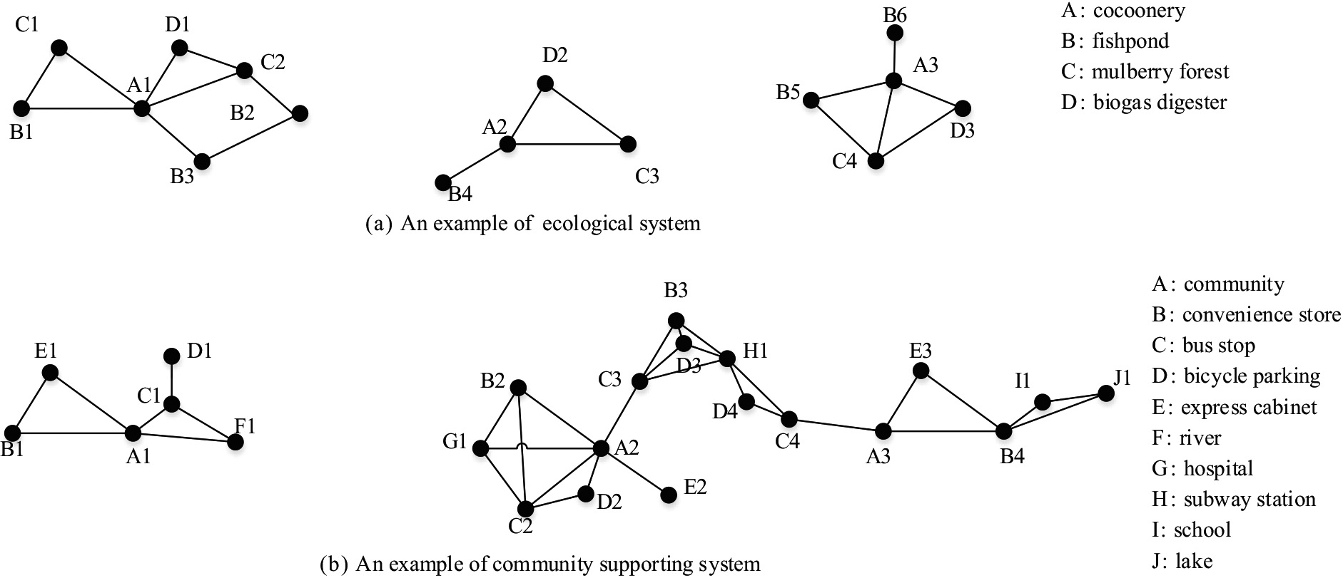(a) suggests there exists the strongly correlated feature set {cocoonery, fishpond, mulberry forest, biogas digester]}. Fig. (b) suggests there exists the strong correlated feature set {community, convenience store, bus stop, bicycle parking}.

Second, the prevalence of a pattern is generally measured by the participation index [8]. Checklists for the participation index always depend on the co-location instance. For a pattern, its instance is generally defined as a clique that carries only all of the features of the pattern in the spatial neighbor relationship graph [9]. For example, {A1, B1, C1} is an instance of {A, B, C} in Fig. 1a. The set that comprises all instances of each co-location pattern is called its table instance. Along this line, the participation ratio of a feature in a pattern is defined as the ratio of distinct instances of the feature appearing in the pattern’s table instance to all distinct instances of the feature, and then, the participation index is the minimum participation ratio among the features of the pattern [8]. If the participation index of a pattern is not less than the given threshold, we say that the pattern is prevalent. A prevalent pattern is also called a co-location pattern. As illustrated in Fig. 1a, the participation index of pattern {A, B, C} is

\min\{2/6,2/3,2/4\}=1/3

because its table instance is {{A1, B1, C1}, {A3, B5, C4}}. Once the given threshold is not greater than 1/3, it is prevalent. Since all possible prevalent patterns are exponential to the feature count, the majority of scholars pay attention to pruning strategies [10, 11] of candidate patterns, such as the anti-monotonicity of the participation index [8].

1.2 Motivation

Since the majority of existing models in this field only account for clique relationships among instances, some interesting spatial correlations among features can be neglected in practice [11]. Therefore, the sub-prevalent pattern based on the star relationship is introduced in [12]. A star participation instance (i.e., a star relationship) is a set that comprises instances where each instance is a neighbor of the centric instance. However, the neglect of interesting patterns has just been mitigated.

For example, Fig. 1a locally suggests a famous interesting ecological system named mulberry dike-pond agriculture in the Yangtze River Delta [13]. It is acknowledged that the cocoonery (A), fishpond (B), mulberry forest (C) and biogas digester (D) are strong cooccurrence sites in mulberry dike-pond agriculture. However, it is difficult to obtain the corresponding pattern {A, B, C, D} from the spatial neighbor relationship graph shown in Fig. 1a with either the classical co-location pattern or the sub-prevalent pattern.

Similarly, in urban planning, a community (A) usually leads instances of convenience stores (B), bus stops (C), bicycle parking (D), and express cabinets (E), as shown in Fig. 1b. Traditional models based on clique or star relationships also tend to neglect the corresponding co-location pattern {A, B, C, D, E}.

Interestingly, the members of each instance pair can be reachable to each other in one (or two steps across the centric instance in shortest paths) in a clique (or star) relationship. Therefore, the $l$ -reachability clique, in which the members of each instance pair can be reachable to each other in $l$ steps, is presented. Furthermore, the $l$ -reachability co-location pattern based on the $l$ -reachability clique is introduced in this paper. For example, in Fig. 1a, {A1, B1, B2, B3, C1, C2, D1} is a 3-reachability clique. Borrowing from a classical prevalence index [8], {A, B, C, D} can be prevalent even if the prevalence threshold is set to 1. Since a clique must be a 1-reachability clique and a star neighborhood instance must be a 2-reachability clique, the $l$ -reachability co-location pattern is an extension of the existing models.

1.3 Roadmap

Since the $l$ -reachability co-location pattern is an extension of co-location patterns, we will try to convert $l$ -reachability co-location pattern mining into co-location pattern mining. Given a spatial neighbor relationship graph and a step length $l$ , if the members of any instance pair can be reachable to each other in $l$ steps, connect them (e.g., solid lines for initialization and dotted lines for update). In other words, the updated graph (called the $l$ -reachability neighbor relationship graph in this paper) can be regarded as a classical spatial neighbor relationship graph if initialized edges and updated edges are treated without distinction. Obviously, with similar prevalence metrics, an $l$ -reachability co-location pattern in a spatial neighbor relationship graph must be a co-location pattern in the corresponding $l$ -reachability neighbor relationship graph, and vice versa. Thus, $l$ -reachability co-location pattern mining can be converted into co-location pattern mining.

Similar to co-location patterns, we will prove $l$ -reachability co-location patterns satisfy Apriori property. Thus, maximal $l$ -co-location pattern can represent all $l$ -reachability co-location patterns. A maximal $l$ -reachability co-location pattern is an $l$ -reachability co-location pattern whose true super sets cannot be prevalent. Thus, we focus in mining maximal $l$ -reachability co-location patterns in this paper.

The baseline method updates the spatial neighbor relationship graph into the $l$ -reachability neighbor relationship graph and then finds candidate maximal co-location patterns (i.e., candidate maximal $l$ -reachability co-location patterns) based on size-2 co-location patterns (i.e., size-2 $l$ -reachability co-location patterns) in the updated graph with no discrimination between dashed lines and solid lines. Furthermore, it tends to check candidate maximal $l$ -reachability co-location patterns one by one in a size-wise way. Namely, once a candidate size- $k$ pattern is refused, all of its size-( $k$ -1) subsets will wait for validation. Figure 2a shows the baseline method for maximal $l$ -reachability co-location pattern mining.

Figure 2.

Comparison of our frameworks. The baseline method bridges the maximal 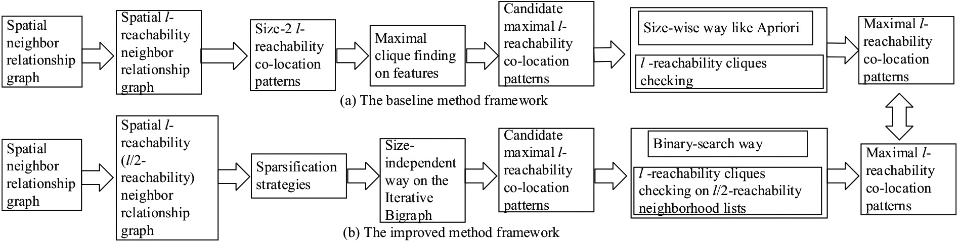$l$ -reachability co-location pattern mining with the classical co-location pattern mining. The improved method is workable both in maximal $l$ -reachability co-location pattern mining and in classical co-location pattern mining.

Fortunately, the baseline method to mine maximal $l$ -reachability co-location patterns can be improved.

First, since it is much easier to mine co-location patterns in a sparser spatial neighbor relationship graph (or $l$ -reachability neighbor relationship graph), some sparsification strategies are briefly introduced to shorten star neighborhood lists (or star $l$ -reachability neighborhood lists). Taking a strategy as an example, for each instance neighbor pair $i_{u}$ and $i_{v}$ , $i_{v}$ can be removed from $i_{u}$ ’s star neighborhood list (or $l$ -reachability neighborhood list) $N_{l}(i_{u})$ when the size of the corresponding pattern of $N_{l}(i_{u})$ is greater than or equal to the $N_{l}(i_{u})$ ’s according to the symmetry of spatial neighbor relationships (or $l$ -reachability neighbor relationships).

Second, candidate maximal co-location patterns (or candidate maximal $l$ -reachability co-location patterns) generated from size-2 co-location patterns (or size-2 $l$ -reachability co-location patterns) can be size-longer than maximal co-location patterns (or maximal $l$ -reachability co-location patterns). Thus, a size-independent way to generate candidate maximal co-location patterns (or candidate maximal $l$ -reachability co-location patterns) is introduced based on a bi-graph.

Third, since the number of subsets of a size- $k$ pattern is $2^{k}$ , it could be time-consuming if a size- $k$ candidate maximal co-location pattern (or candidate maximal $l$ -reachability co-location pattern) is checked in a size-wise way from $k$ to 2. Therefore, a binary-search way to check candidate maximal co-location patterns (or candidate maximal $l$ -reachability co-location patterns) is introduced.

Fourth, checking the prevalence (e.g., participation index) of each candidate maximal co-location pattern (or candidate maximal $l$ -reachability co-location pattern) should check cliques (or $l$ -reachability cliques) first. For example, [14] checks each size- $k$ candidate maximal co-location pattern in a join-based way [8] following a size-wise way from 1 to $k$ . In this paper, a natural $l$ -reachability clique named the $\lfloor l/2\rfloor$ -reachability neighborhood list is introduced, and then, the $l$ -reachability clique validation can be reduced.

In other words, the baseline method is improved, as shown in Fig. 2b. First, the $\lfloor l/2\rfloor$ -reachability neighborhood lists of instances are generated, and then, $l$ -reachability neighborhood lists can be captured in a join-based way. Second, some sparsification strategies are suggested to shorten $l$ -reachability neighborhood lists. Third, candidate maximal $l$ -reachability co-location patterns are acquired in a size-independent way on a bi-graph. Last, each candidate maximal $l$ -reachability co-location pattern is checked in a binary search way on $\lfloor l/2\rfloor$ -reachability neighborhood lists.

1.4 Main contributions

In summary, the main contributions of this paper include the following:

1)
A more general $l$ -reachability co-location pattern based on the $l$ -reachability clique is proposed. A model to convert the maximal $l$ -reachability co-location pattern mining into maximal co-location pattern mining is introduced, and then, a baseline method is proposed.
2)
To improve maximal $l$ -reachability co-location pattern mining, some sparsification strategies are briefly introduced to shorten $l$ -reachability neighborhood lists, and then, candidate maximal $l$ -reachability co-location patterns are iteratively acquired in a size-independent way on bi-graphs. Furthermore, candidate maximal $l$ -reachability co-location patterns are checked in a binary search way with a natural $l$ -reachability clique called the $\lfloor l/2\rfloor$ -reachability neighborhood list. These methods are also locally workable for classical co-location pattern mining when $l=1$ .
3)
Extensive experiments on both real and synthetic data sets show the superiority of the $l$ -reachability co-location pattern as well as the efficiency of the proposed algorithms.

The remainder of this paper is organized as follows. In Section 2, related works are reviewed. In Section 3, the $l$ -reachability co-location pattern is defined based on the $l$ -reachability clique. Moreover, a baseline method for maximal $l$ -reachability co-location pattern mining is proposed. In Section 4, sparsification strategies, $\lfloor l/2\rfloor$ -reachability neighborhood lists, a size-independent method on bi-graphs, and a binary search method are proposed to improve the baseline method. Section 5 analyses the effectiveness and efficiency of the proposed $l$ -reachability co-location pattern and mining algorithms on both synthetic and real-world data sets. Finally, the main work of this paper is summarized and prospected.
2. Related works

The co-location pattern mining has got its own since the concept was firstly introduced by Shashi Shekhar Huang [15]. The traditional mining model generally includes three steps whatever in classical or uncertain data sets [16, 17, 18]. First, the neighbor relationship generating. Second, the prevalence check of patterns. Third, the secondary mining for user interest.

The neighbor relationships between spatial instances are generally driven by distance thresholds [19] or nearest neighbors [20] with static or dynamic models [21]. Moreover, there are some variants, such as Delaunay triangulation [22] and so on [23, 24]. We focus on reachability of instances in given basic neighbor relationship graphs but not the generation of graphs in this paper. A spatial neighbor relationship graph is generally materialized by star or clique neighborhood lists [12, 25].

For specific applications, some prevalence metrics [5, 6, 26, 27] have been defined for such as rare feature finding, overlap clique partitioning. The most popular index is the participation index [8], which is followed in this paper.

The methods of mining co-location patterns can be mainly classified into three groups. The first group exploits an Apriori-like method to generate prevalent patterns with considerable time to check co-location instances [8, 28, 29]. This size-wise manner makes approaches in this group inefficient in obtaining longer-size patterns.

The second group suggests using maximal cliques [25, 30, 31] in the spatial neighbor relationship graph to discover co-location patterns. Maximal cliques can be regarded as transactions, and then association analysis methods such as Apriori [19] and FP-growth [32] can come in handy. However, maximal clique finding is an NP-hard problem.

The third one first generates candidate maximal co-location patterns [33, 14, 34] and then checks their prevalence. A candidate maximal co-location pattern is a pattern whose true super sets cannot be prevalent according to some properties, such as the Apriori property. [33] first finds all sub-prevalent patterns (called clique candidates on star candidates in the original text) on star neighborhood lists with a modified FP-tree.

Similarly, [14] finds candidate maximal co-location patterns on MCP trees (similar to the FP tree). A candidate maximal co-location pattern corresponds to the longest path of an MCP tree. [34] finds maximal cliques on a size-2 co-location pattern graph with a degenerated order list [31], and then, each maximal clique is regarded as a candidate maximal co-location pattern. Once the candidate maximal co-location patterns have been generated, the third group tends to check each of them in a size-wise way. For example, if a size- $k$ candidate maximal co-location pattern is refused, all of its size-( $k$ -1) subsets can replace it as new candidate maximal co-location patterns.

The first group is troubled with long-size pattern finding, and the second group is limited to the maximal clique finding problem. Since $l$ -reachability cliques can lead to longer-size $l$ -reachability co-location patterns, the third is followed in this paper. Thus, our task focuses on mining maximal $l$ -reachability co-location patterns (i.e., $l$ -reachability co-location patterns whose true supersets cannot be prevalent) rather than all $l$ -reachability co-location patterns with their prevalence indexes. Since [33, 14] serve for top- $k$ co-location patterns and top- $k$ -size maximal co-location patterns, a baseline method is proposed with the help of [34] as shown in Fig. 2.

3. Maximal $l$ -reachability co-location pattern

In this section, the $l$ -reachability clique and the $l$ -reachability co-location pattern are introduced in sequence. Moreover, a baseline method to mine maximal $l$ -reachability co-location patterns is proposed.

3.1 $l$ -reachability co-location pattern

For ease of exposition, suppose that we have a spatial neighbor relationship $R$ on an instance set $I(I=\{i_{u}\mid i_{u}\textit{ is an instance}\})$ that carries spatial features $F(F=\{f_{i}\mid f_{i}\textit{ is a class label}\})$ . Then, $G=(I,R)$ is a spatial neighbor relationship graph (generally an undigraph) where edges connect each pairwise neighbor instance.

( $l$ -reachability neighborhood list).

Given a graph $G=(I,R)$ of a spatial dataset $D$ , for any instance $i_{u}(i_{u}\in I)$ , the $l$ -reachability neighborhood list of $i_{u}$ (denoted $N_{l}(i_{u})$ ) is a set that comprises instances that can be reachable to $i_{u}$ in $l$ steps (i.e., across not more than $l$ -1 instances in shortest paths) in $G$ . Namely,

$\displaystyle N_{l}(i_{u})=\{i_{v}\mid i_{v}\in I\wedge\mid sp(i_{u},i_{v})% \mid\leqslant l\}$

where $\mid sp(i_{u},i_{v})\mid$ returns the length of any shortest path between $i_{u}$ and $i_{v}$ in $G$ . Specifically, $N_{0}(i_{u})=\{i_{u}\}$ . The set that comprises all $l$ -reachability neighborhood lists is denoted $Ns_{l}$ .

Each instance in $N_{l}(i_{u})$ is called an $l$ -reachability neighbor of $i_{u}$ . Given any instance pair $i_{u}$ and $i_{v}$ , it is easy to understand that $i_{v}$ is an $l$ -reachability neighbor of $i_{u}$ if and only if $i_{u}$ is an $l$ -reachability neighbor of $i_{v}$ . Namely, $i_{v}\in N_{l}(i_{u})\Leftrightarrow i_{u}\in N_{l}(i_{v})$ . In other words, the $l$ -reachability neighbor relationship set $R_{l}(R_{l}=\{\langle i_{u},i_{v}\rangle\mid i_{u}\in I\wedge i_{v}\in N_{l}(i% _{u})\})$ satisfies symmetry (i.e., $R_{l}=\{(i_{u},i_{v})\mid i_{u}\in I\wedge i_{v}\in N_{l}(i_{u})\})$ ).

( $l$ -reachability clique).

Given a spatial neighbor relationship graph $G=(I,R)$ of a spatial dataset $D$ , let $I^{\prime}$ be a nonempty subset of $I$ ( $I^{\prime}\subseteq I$ ). If the members of any instance pair in $I^{\prime}$ can be reachable to each other in $l$ steps in $G$ , $I^{\prime}$ is called an $l$ -reachability clique in $G$ . Namely, $I^{\prime}(I^{\prime}\subseteq I)$ is an $l$ -reachability clique if and only if

$\displaystyle(\forall i_{u}\in I^{\prime})(\forall i_{v}\in I^{\prime})(i_{u}% \in N_{l}(i_{v})\wedge i_{v}\in N_{l}(i_{u}))$ (1)

(Nestedness of $l$ -reachability cliques).

Given a nonnegative integer $l$ , assuming that there is an $l$ -reachability clique in $G$ denoted $C_{l}$ , any subset of $C_{l}$ must be an $l$ -reachability clique in $G$ . Namely, ( $\forall C^{\prime}_{l}\subseteq C_{l}$ ) ( $C^{\prime}_{l}$ is an $l$ -reachability clique) is true.

Proof..

Given a non-negative integer $l$ , let $C_{l}$ be an $l$ -reachability clique in $G$ . Therefore, any subset of $C_{l}$ must be an $l$ -reachability clique because the members of each instance pair in $C_{l}$ can be reachable to each other in $l$ steps in $G$ , let alone each instance pair in a subset of $C_{l}$ . ∎

Importantly, Lemma 1 is true only when the reachability is considered in the whole spatial neighbor relationship graph $G$ but not in its subgraphs.

.

In Fig. 1a, {A1, B1, B2, B3, C1, C2, D1} is a 3-reachbility clique. In addition, any of its subsets is also a 3-reachability clique. More specifically, {B1, D1} is a 3-reachability clique since B1 (or D1) can be reachable to D1 (or B1) across A1 in Fig. 1a.

Obviously, a clique must be a 1-reachability clique and vice versa. Since the members of any instance pair in a star neighborhood instance can be reachable to each other directly or across the centric instance, each star neighborhood instance must be a 2-reachability clique. In other words, the $l$ -reachability clique is an extension of both the clique relationship and the star relationship.

( $l$ -reachability instance).

Given a step length $l$ and a spatial neighbor relationship graph $G=(I,R)$ , let $p(p\subseteq F)$ be a non-empty feature set. An $l$ -reachability clique denoted $C_{l}$ , whose corresponding pattern (i.e., $\{\textit{fea}(o)\mid o\in C_{l}\}$ where $\textit{fea}(o)$ returns the feature carried by $o$ ) is $p$ with distinct features, is called an $l$ -reachability instance of $p$ . The set containing all $l$ -reachability instances of $p$ is called the $l$ -reachability table instance of $p$ (denoted $\textit{ins}_{l}(p)$ ).

.

In Fig. 1a, {A1, B1, C1, D1} is a 3-reachability instance of {A, B, C, D}. Although {A1, B1, B2, B3, C1, C2, D1} is a 3-reachability clique, it is not a 3-reachability instance of {A, B, C, D} because duplicate features B (B1, B2, B3) and C (C1, C2) exist.

( $l$ -reachability participation ratio).

Given a step length $l$ and a spatial neighbor relationship graph $G=(I,R)$ , a nonempty feature set $p(p\subseteq F)$ and a feature $f_{i}$ in $p(f_{i}\in p)$ , the $l$ -reachability participation ratio of $f_{i}$ in $p$ , denoted $PR_{l}(p,f_{i})$ , is the ratio of distinct instances of $f_{i}$ appearing in the $l$ -reachability table instance of $p$ to all distinct instances of $f_{i}$ . Namely,

$\displaystyle PR_{l}(p,f_{i})=\frac{\mid\{x\mid(\exists y\in ins_{l}(p))(x\in y% \wedge\textit{fea}(x)=f_{i})\}\mid}{\mid\{x\mid x\in I\wedge\textit{fea}(x)=f_% {i}\}\mid}$ (2)

.

In Fig. 1a, $PR_{3}$ ({A, B, C, D}) $=$ 4/4 $=$ 1.

( $l$ -reachability participation index).

Given a step length $l$ and a nonempty feature set $p(p\subseteq F)$ , the $l$ -reachability participation index of $p$ is the minimum $l$ -reachability participation ratio of each feature in $p$ . Namely,

$\displaystyle PI_{l}(p)=\min_{f_{i}\in p}PR_{l}(p,f_{i})$ (3)

( $l$ -reachability co-location pattern).

Given a step length $l$ , a nonempty feature set $p(p\subseteq F)$ and an $l$ -reachability prevalence threshold $\textit{min}\_pi_{l}(0<\textit{min}\_pi_{l}\leqslant 1)$ ; if the $l$ -reachability participation index of $p$ is not less than $\min\_pi_{l}$ , we say that $p$ is prevalent. Then, it is called an $l$ -reachability co-location pattern. The set that comprises all $l$ -reachability co-location patterns is denoted $\textit{FPs}_{l}$ ( $\textit{FPs}_{l}=\{p\mid p\subseteq F\wedge PI_{l}(p)\geqslant\textit{min}\_pi% _{l}\}$ ).

.

In Fig. 1a, $PI_{3}$ ({A, B, C, D}) $=$ $\min$ {3/3, 6/6, 4/4, 3/3} $=$ 1. {A, B, C, D} is a 3-reachability co-location pattern even if the prevalence threshold $\textit{min}\_pi_{l}$ is equal to 1.

Similar to the $l$ -reachability clique, the $l$ -reachability co-location pattern is an extension of the existing models, such as the co-location pattern and the sub-prevalent pattern.

(Anti-monotonicity of $PR_{l}(p,f_{i})$ and $PI_{l}(p)$ ).

Let $p$ and $p^{\prime}$ be two nonempty feature sets ( $p^{\prime}\subseteq p\subseteq F$ ). For each spatial feature $f_{i}$ in $p^{\prime}$ ( $f_{i}\in p^{\prime}$ , absolutely $f_{i}\in p$ ), $PR_{l}(p^{\prime},f_{i})\geqslant PR_{l}(p,f_{i})$ . Moreover, $PI_{l}(p^{\prime})\geqslant PI_{l}(p)$ .

Proof..

Assuming that $f_{i}\in p^{\prime}$ and $p^{\prime}\subseteq p$ , $\textit{ins}_{l}(p^{\prime})$ and $\textit{ins}_{l}(p)$ are $l$ -reachability table instances of $p^{\prime}$ and $p$ , respectively.

Certainly, $(\forall C_{l}\in\textit{ins}_{l}(p))(\exists i_{u}\in C_{l})(\textit{fea}(i_{% u})=f_{i})\Rightarrow(\exists C^{\prime}_{l}\subseteq C_{l})(i_{u}\in C^{% \prime}_{l}\in\textit{ins}_{l}(p^{\prime}))$ according to Lemma 1.

Thus, $PR_{l}(p^{\prime},f_{i})\geqslant PR_{l}(p,f_{i})$ .

Furthermore, $PI_{l}(p^{\prime})=\min_{f_{i}\in p^{\prime}}PR_{l}(p^{\prime},f_{i})\geqslant% \min_{f_{i}\in p^{\prime}}PR_{l}(p,f_{i})\geqslant\\ \min\{\min_{f_{i}\in p^{\prime}}PR_{l}(p,f_{i}),\min_{f_{j}\in p-p^{\prime}}PR% _{l}(p,f_{j})\}=PI_{l}(p)$ . ∎

Lemma 2 declares that the Apriori property is accepted by the $l$ -reachability co-location pattern. That is, if a nonempty feature set $p(p\subseteq F)$ is an $l$ -reachability co-location pattern, then the same property holds for any of its true subsets. In contrast, if a nonempty feature set $p(p\subseteq F)$ is not an $l$ -reachability co-location pattern, then the same property does not hold for any of its supersets.

(Maximal $l$ -reachability co-location pattern).

Given an $l$ -reachability co-location pattern $p$ and an $l$ -reachability prevalence threshold $\textit{min}\_pi_{l}$ ; if any true superset of $p$ is not prevalent, $p$ is called a maximal $l$ -reachability co-location pattern. The set that comprises all maximal $l$ -reachability co-location patterns is denoted $\textit{MCPs}_{l}$ .

$\displaystyle\textit{MCPs}_{l}=\{p\mid p\subseteq F\wedge PI_{l}(p)\geqslant% \textit{min}\_pi_{l}\wedge(\not\exists p^{\prime}\supset p)(PI_{l}(p^{\prime})% \geqslant\textit{min}\_pi_{l})\}$ (4)

.

In Fig. 1a, {A, B, C, D} is a maximal 3-reachability co-location pattern, but neither any true subset nor any true superset occurs when $\textit{min}\_pi_{l}=1$ .

3.2 A baseline method

Figure 3.

An example of the baseline method.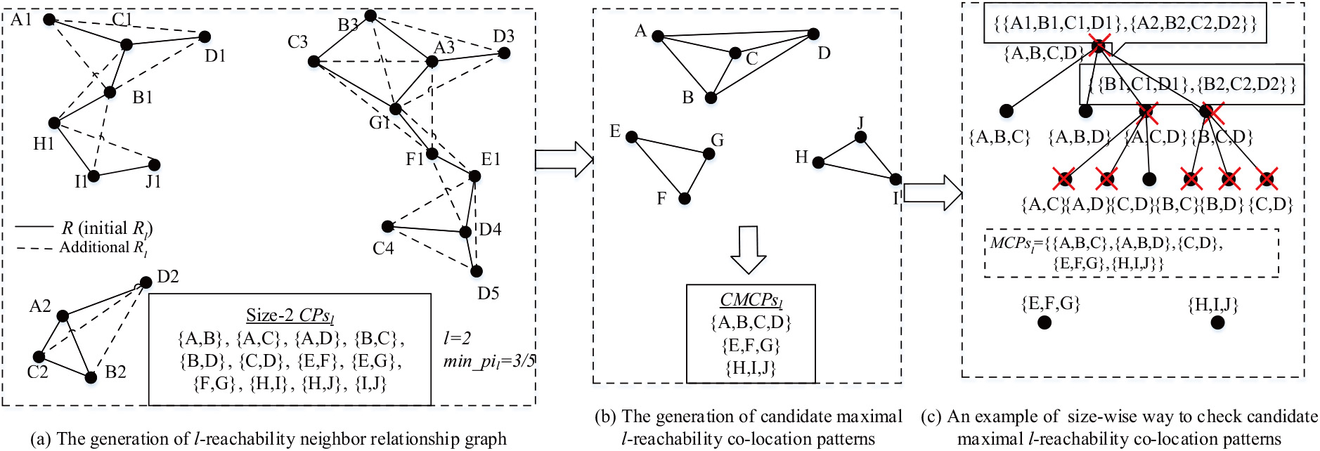

Learning from traditional co-location pattern mining approaches, $l$ -reachability co-location pattern mining can be decomposed into two steps once a spatial neighbor relationship graph $G=(I,R)$ has been given. First, if there is a shortest path whose length is not longer than the step length $l$ between any instance pair in $G=(I,R)$ , a new dotted line connects them, as shown in Fig. 3a. The updated graph is called the $l$ -reachability neighbor relationship graph $G^{\prime}=(I,R_{l})$ . An $l$ -reachability clique is a clique without distinction once nondiscrimination is present for edges of either a solid line or a dotted line in the $l$ -reachability neighbor relationship graph. Thus, an $l$ -reachability co-location pattern in a spatial neighbor relationship graph is a co-location pattern in the corresponding $l$ -reachability neighbor relationship graph with the same prevalence threshold. Therefore, $l$ -reachability co-location pattern mining can be converted into co-location pattern mining when the input is replaced by the $l$ -reachability neighbor relationship graph. Note that there exists a maximal co-location pattern mining method [34], and a baseline method can be proposed.

[h] : The Baseline Method ( $B M$ ))[1] $G=(I,R)$ , $l$ , $\textit{min}\_pi_{l}$ . $\textit{MCPs}_{l}$ . $R_{l}=R$ $i_{u}\in I$ $i_{v}\in I$ $\mid sp(i_{u},i_{v})\mid\leqslant l$ $R_{l}\cup=\{<i_{u},i_{v}>\}$ //Definition 1. $G=(I,R_{l})$ $f_{0}\in F$ $f_{1}\in F$ $\textit{pi\_check}(G,\{f_{0},f_{1}\},\min\_pi_{l})$ $P^{\prime\prime}\cup=\{f_{0},f_{1}\}$ //Get size-2 $\textit{FPs}_{l}$ . $G^{\prime}=(F,P^{\prime\prime})$ //Create a graph for size-2 $\textit{FPs}_{l}$ . $\textit{CMCPs}_{l}=\textit{Bron\_Kerbosch}(G^{\prime})$ //Lemma 2. $\textit{CMCPs}_{l}$ $p=\textit{CMCPs}_{l}.\textit{pop}()$ //Check $p$ . $\textit{pi\_check}(G,p,\min\_pi_{l})$ $\textit{MCPs}_{l}\cup=\{p\}$ //Definition 7. $\textit{CMCPs}_{l}\cup=\textit{combinations}(p,\mid p\mid-1)$ //Replace $p$ with its size-( $\mid p\mid-1$ ) subsets. $\textit{MCPs}_{l}=\max(\textit{MCPs}_{l})$ //Clean $\textit{MCPs}_{l}$ .

Algorithm 3 works for maximal $l$ -reachability co-location patterns from a spatial neighbor relationship graph. The steps from Step 3 to Step 3 generate the $l$ -reachability neighbor relationship graph from the input neighbor relationship graph. The steps from Step 3 to Step 3 obtain candidate maximal $l$ -reachability co-location patterns from size-2 $l$ -reachability co-location patterns. The steps from Step 3 to Step 3 check candidate maximal $l$ -reachability co-location patterns.

Since the generation of the $l$ -reachability neighbor relationship $R_{l}$ is easier than the generation of transitive closure of spatial neighbor relationship $R$ , the time complexity of the steps from Step 3 to Step 3 will not be higher than $O(n^{3})$ with the help of Warshall’s algorithm [35], where $n$ represents the size of instance set $\mid I\mid$ . Steps from Step 3 to Step 3 are used to generate a size-2 $l$ -reachability co-location pattern graph $G^{\prime}$ , as shown in Fig. 3b. It takes $O(e^{2})$ , where $e$ represents the edge number in $G^{\prime}$ . Unfortunately, Step 3 is an NP-hard problem because it is essentially a maximal clique finding problem on the size-2 $l$ -reachability co-location pattern graph [33], as shown in Fig. 3b. The steps from Step 3 to Step 3 could be exponential, which suggests that all subsets of each candidate pattern should be checked in a size-wise way [33], as shown in Fig. 3c. Therefore, the baseline method Algorithm 3 is time-consuming for Step 18 and Step 19. An improved method will be proposed in the next section.

4. The improved method

In this section, a natural $l$ -reachability clique, some sparsification strategies, iterative bi-graphs, and a binary-search method are introduced in sequence to efficiently mine maximal $l$ -reachability co-location patterns.

4.1 A natural $l$ -reachability clique

Since steps from Step 3 to Step 3 in Algorithm 3 follow an Apriori-like way from 1 to $l$ to generate an $l$ -reachability neighborhood list of each instance, we suggest improving it in a reversed binary-search way.

(A natural $l$ -reachability clique).

Given a spatial neighbor relationship graph $G=(I,R)$ and a step length $l$ , the $\lfloor l/2\rfloor$ -reachability neighborhood list of any instance must be an $l$ -reachability clique.

Proof..

Given a spatial neighbor relationship graph $G=(I,R)$ and a step length $l$ , for each instance $i_{u}(i_{u}\in I)$ , any instance $i_{v}$ in $i_{u}$ ’s $\lfloor l/2\rfloor$ -reachability neighborhood list ( $i_{v}\in N_{\lfloor l/2\rfloor}(i_{u})$ ) can be reachable to instance $i_{u}$ in $\lfloor l/2\rfloor$ steps. In other words, any pairwise instances in $N_{\lfloor l/2\rfloor}(i_{u})$ can be reachable to each other in $l$ (i.e., $\lfloor l/2\rfloor$ + $\lfloor l/2\rfloor\leqslant l$ ) steps with the help of $i_{u}$ . Therefore, $N_{\lfloor l/2\rfloor}(i_{u})$ must be an $l$ -reachability clique. ∎

.

In Fig. 3a, since $N_{\lfloor 2/2\rfloor}$ (C1) $=$ {A1, B1, C1, D1}, {A1, B1, C1, D1} is a 2-reachability clique.

(Reversed binary-search of $N_{l}(i_{u})$ ).

Given a spatial neighbor relationship graph $G=(I,R)$ and a step length $l$ , for any instance $i_{u}$ ( $i_{u}\in I$ ), its $l$ -reachability neighborhood list can be generated in a reversed binary-search way. Namely,

$\displaystyle N_{l}(i_{u})=\bigcup_{i_{w}\in\cup_{i_{v}\in N_{\lfloor l/2% \rfloor}(i_{u})}N_{\lfloor l/2\rfloor}(i_{v})}N_{l-2*\lfloor l/2\rfloor}(i_{w})$ (5)

Proof..

Given a spatial neighbor relationship graph $G=(I,R)$ and a step length $l$ , for an instance denoted $i_{u}$ ( $i_{u}\in I$ ), its 0-reachability neighborhood list

$\displaystyle N_{0}(i_{u})=\bigcup_{i_{w}\in\cup_{i_{v}\in N_{\lfloor 0/2% \rfloor}(i_{u})}N_{\lfloor 0/2\rfloor}(i_{v})}N_{0-2*\lfloor 0/2\rfloor}(i_{w})$

Letting $l=k$ ,

$\displaystyle N_{k}(i_{u})=\bigcup_{i_{w}\in\cup_{i_{v}\in N_{\lfloor k/2% \rfloor}(i_{u})}N_{\lfloor k/2\rfloor}(i_{v})}N_{k-2*\lfloor k/2\rfloor}(i_{w})$

Thus,

$\displaystyle N_{k+1}(i_{u})=\cup_{i_{x}\in N_{k}(i_{u})}N_{1}(i_{x})=\bigcup_% {i_{x}\in\bigcup_{i_{w}\in\cup_{i_{v}\in N_{\lfloor k/2\rfloor}(i_{u})}N_{% \lfloor k/2\rfloor}(i_{v})}N_{k-2*\lfloor k/2\rfloor}(i_{w})}N_{1}(i_{x})$

If $k=2m$ ( $m$ is a nonnegative integer), then let $l=2m+1=k+1$ .

$\displaystyle\cup_{i_{x}\in N_{2m}(i_{u})}N_{1}(i_{x})=\bigcup_{\cup_{i_{w}\in% \cup_{i_{v}\in N_{\lfloor 2m/2\rfloor}(i_{u})}N_{\lfloor 2m/2\rfloor}(i_{v})}N% _{2m-2*\lfloor 2m/2\rfloor}(i_{w})}N_{1}(i_{x})=\bigcup_{\cup_{i_{w}\in\cup_{i% _{v}\in N_{m}(i_{u})}N_{m}(i_{v})}N_{0}(i_{w})}N_{1}(i_{x})=\bigcup_{i_{w}\in% \cup_{i_{v}\in N_{m}(i_{u})}N_{m}(i_{v})}N_{1}(i_{w})=\bigcup_{i_{w}\in\cup_{i% _{v}\in N_{\lfloor l/2\rfloor}(i_{u})}N_{\lfloor l/2\rfloor}(i_{v})}N_{l-2*% \lfloor l/2\rfloor}(i_{w})$

If $k=2m+1$ ( $m$ is a nonnegative integer), then let $l=2m+2=k+1$ .

$\displaystyle\cup_{i_{x}\in N_{2m+1}(i_{u})}N_{1}(i_{x})=\bigcup_{\cup_{i_{w}% \in\cup_{i_{v}\in N_{\lfloor(2m+1)/2\rfloor}(i_{u})}N_{\lfloor(2m+1)/2\rfloor}% (i_{v})}N_{(2m+1)-2*\lfloor(2m+1)/2\rfloor}(i_{w})}N_{1}(i_{x})=\bigcup_{\cup_% {i_{w}\in\cup_{i_{v}\in N_{m}(i_{u})}N_{m}(i_{v})}N_{1}(i_{w})}N_{1}(i_{x})=% \bigcup_{\cup_{i_{w}\in\cup_{i_{v}\in N_{m}(i_{u})}N_{m}(i_{v})}N_{2}(i_{w})}N% _{0}(i_{x})=\bigcup_{i_{w}\in\cup_{i_{v}\in N_{m+1}(i_{u})}N_{m+1}(i_{v})}N_{0% }(i_{w})=\bigcup_{i_{w}\in\cup_{i_{v}\in N_{\lfloor l/2\rfloor}(i_{u})}N_{% \lfloor l/2\rfloor}(i_{v})}N_{l-2*\lfloor l/2\rfloor}(i_{w})$

∎

Lemma 4 declares that $l$ -reachability neighborhood lists can be detected in a reversed binary search way to avoid the size-wise way. Furthermore, Lemma 3 and Lemma 4 declare that instances in the $l$ -reachability neighborhood list of an instance $i_{u}$ can be partitioned into two subsets. The first subset is an $l$ -reachability clique (i.e., the $\lfloor l/2\rfloor$ -reachability neighborhood list of $i_{u}$ ). Therefore, the format of the $l$ -reachability neighborhood list of an instance $i_{u}$ can be expressed as $N_{l}(i_{u})=\{N_{\lfloor l/2\rfloor}(i_{u}),N_{l}(i_{u})-N_{\lfloor l/2% \rfloor}(i_{u})\}$ .

For example, in Fig. 3a, $N_{2}$ (C1) $=$ {{A1, B1, C1, D1},ø} and $N_{2}$ (A3) $=$ {{A3, B3, D3, G1}, {C3, F1}}. In the modified $N_{l}(i_{u})$ , there exists an inter-order between $N_{\lfloor l/2\rfloor}(i_{u})$ and $N_{l}(i_{u})-N_{\lfloor l/2\rfloor}(i_{u})$ but not intra-order.

It is acknowledged that mining co-location patterns over a very large-scale sparse spatial dataset is much faster than in a denser dataset [31], and we will briefly introduce sparsification strategies to make the $l$ -reachability neighbor relationship graph sparser.

First, it is understandable that edges whose endpoints are not related to any size-2 $l$ -reachability co-location pattern cannot contribute to any size-longer $l$ -reachability co-location patterns according to Lemma 2. Second, if an instance $i_{u}$ can be reachable to another instance $i_{v}$ in $l$ steps, $i_{v}$ must also be reachable to $i_{u}$ in $l$ steps. Thus, removing $i_{u}$ (or $i_{v}$ ) from the $l$ -reachability neighborhood list of $i_{v}$ (or $i_{u}$ ) will not lose the $l$ -reachability neighbor relationship between $i_{u}$ and $i_{v}$ . Thus, alternatively removing $l$ -reachability neighbor pairs by the symmetry of $l$ -reachability neighbor relationships is impervious to $l$ -reachability cliques. Since an $l$ -reachability instance must be an $l$ -reachability clique, the removal is acceptable. Assume that we are given an instance $i_{u}$ ( $i_{u}\in I$ ). Then, for instance, $i_{v}$ in $N_{l}(i_{u})$ , $i_{v}$ can be removed from $N_{l}(i_{u})$ if the size of $N_{l}(i_{u})$ ’s corresponding pattern is greater than or equal to that of $N_{l}(i_{v})$ ’s. In contrast, $i_{u}$ can be removed from $N_{l}(i_{v})$ . Third, assume that we are given the $l$ -reachability neighborhood list of an instance $N_{l}(i_{u})$ with corresponding pattern $p$ . Let $p^{\prime}$ be an $l$ -reachability co-location pattern, and there exists an $l$ -reachability clique $C_{l}$ whose corresponding pattern is $p^{\prime}$ in $N_{l}(i_{u})$ . Thus, $p^{\prime}\subseteq p$ . According to Definition 3, if there exist multiple instances that carry the same feature $f_{i}$ , $C_{l}$ can be broken up into size- $\mid p^{\prime}\mid$ subsets whose corresponding pattern set is $p^{\prime}$ . Therefore, $N_{l}(i_{u})$ can be broken into its size- $\mid p\mid$ subsets whose corresponding pattern set is $p$ .

4.2 Iterative bi-graphs

Once $l$ -reachability neighborhood lists have been shortened by sparsification strategies, maximal $l$ -reachability co-location pattern mining can be put on the agenda in a size-independent way.

( $l$ -reachability neighborhood list cluster).

Given an $l$ -reachability neighborhood list set $Ns_{l}$ , then $Ns_{l}$ is grouped by their corresponding patterns. Each group is called an $l$ -reachability neighborhood list cluster. The $l$ -reachability neighborhood list cluster set is denoted as $Cs_{l}$ . A group with a key $k$ is denoted as $Cs_{l}(k)$ .

In detail, the label set of $Cs_{l}$ is denoted keys ( $\textit{keys}=\{\{\textit{fea}(i_{u})\mid i_{u}\in s_{0}\cup s_{1}\}\mid\{s_{0% },s_{1}\}\in Ns_{l}\}$ . Thus,

$\displaystyle Cs_{l}(k)=\left\{\{s_{0},s_{1}\}\mid\{\textit{fea}(i_{u})\mid i_% {u}\in s_{0}\cup s_{1}\}=k,\{s_{0},s_{1}\}\in Ns_{l}\right\}$ (6)

where $k\in\textit{keys}$ .

(Star $l$ -reachability neighborhood instance).

We are given a pattern $p$ and an $l$ -reachability neighborhood list cluster set $Cs_{l}$ whose label set is keys. A star $l$ -reachability neighborhood instance of $p$ is a subset of an $l$ -reachability neighborhood list whose corresponding pattern is $p$ with distinct features. The star $l$ -reachability neighborhood table instance of $p$ is the set that comprises all star $l$ -reachability neighborhood instances of $p$ (denoted $S_{l}(p)$ ). Namely,

$\displaystyle S_{l}(p)=\bigcup_{p\subseteq k,k\in\textit{keys}}\{\{\{\{y_{0}% \mid y_{0}\in x_{0},\textit{fea}(y_{0})\in p\},\{y_{1}\mid y_{1}\in x_{1},% \textit{fea}(y_{1})\in p\}\}\mid$ $\displaystyle\qquad\{x_{0},x_{1}\}\in Cs_{l}(k),\mid\{\{y_{0}\mid y_{0}\in x_{% 0},\textit{fea}(y_{0})\in p\}$ (7) $\displaystyle\qquad\cup\{y_{1}\mid y_{1}\in x_{1},\textit{fea}(y_{1})\in p\}\}% \mid=\mid p\mid\}\}.$

.

There exist two 2-reachability neighborhood list clusters whose labels are {A, B, C, D} and {A, B, C} in Fig. 3a. Moreover, $Cs_{2}$ ({A, B, C, D}) $=$ {{{A1, B1, C1, D1}, ø}, {{C1, D1}, {A1, B1}}, {{A2, B2, C2, D2}, ø}, {{A2, B2, C2}, {D2}}} and $Cs_{2}$ ({A, B, C}) $=$ {{{B1, C1}, {A1}}, {{A3, B3, C3}, ø}, {{B3, C3}, {A3}} after shortening by sparsification strategies. $S_{2}$ ({A, B, C}) $=$ {{{A1, B1, C1}, ø}, {{C1}, {A1, B1}}, {{A2, B2, C2}, ø}, {{B1, C1}, {A1}}, {{A3, B3, C3}, ø}, {{B3, C3}, {A3}}}.

(Upper participation ratio).

Assume that we are given a pattern $p$ , a feature $f_{i}$ ( $f_{i}\in p$ ) and an $l$ -reachability neighborhood list cluster set $Cs_{l}$ whose label set is keys. The upper participation ratio of $f_{i}$ in $p$ (denoted $\textit{UPR}_{l}(p,f_{i})$ ) is defined as the ratio of instances of $f_{i}$ appearing in the star $l$ -reachability table instance of $p$ to instances of $f_{i}$ , namely,

$\displaystyle\textit{UPR}_{l}(p,f_{i})=\frac{\mid\{i_{u}\mid p^{\prime}\in% \textit{keys},p\subseteq p^{\prime},\{s_{0},s_{1}\}\in Cs_{l}(p^{\prime}),i_{u% }\in s_{0}\cup s_{1},\textit{fea}(i_{u})=f_{i}\}\mid}{\mid\{i_{u}\mid i_{u}\in I% ,\textit{fea}(i_{u})=f_{i}\}\mid}$ (8)

(Upper participation index).

Assume that we are given a pattern $p$ ( $p\subseteq F$ ). The upper participation index of $p$ (denoted $\textit{UPI}_{l}(p)$ ) is defined as the minimum upper participation ratio of each feature in $p$ , namely,

$\displaystyle\textit{UPI}_{l}(p)=\min_{f_{i}\in p}\textit{UPR}_{l}(p,f_{i})$ (9)

.

In Fig. 3a, $\textit{UPI}_{2}(\rm{\{A,B,C\}})=\min\{\mid{\rm\{A1,A2,A3\}}\mid/\mid{\rm\{A1,% A2,A3\}}\mid,\mid{\rm\{B1,B2,B3\}}\mid/\mid{\rm\{B1,B2,B3\}}\mid,\mid{\rm\{C1,% C2,C3\}}\mid/\mid{\rm\{C1,C2,C3,C4\}}\mid\}=3/4$ .

(Anti-monotonicity of $\textit{UPR}_{l}(p,f_{i})$ and $\textit{UPI}_{l}(p)$ ).

Assume that we are given two patterns $p$ and $p^{\prime}$ ( $p^{\prime}\subseteq p\subseteq F$ ), any feature $f_{i}$ in $p^{\prime}$ ( $f_{i}\in p^{\prime}$ , and then $f_{i}\in p$ undoubtedly) and an $l$ -reachability neighborhood list cluster set $Cs_{l}$ . The upper participation ratio of $f_{i}$ in $p^{\prime}$ must be equal to or greater than the participation ratio of $f_{i}$ in $p$ , namely,

$\displaystyle(\forall p\subseteq F)(\exists p^{\prime}\subseteq F)(p^{\prime}% \subseteq p)\Rightarrow(\forall f_{i}\in p)(\textit{UPR}_{l}(p^{\prime},f_{i})% \geqslant\textit{UPR}_{l}(p,f_{i}))$ (10)

Furthermore, the upper participation index of $p^{\prime}$ must be equal to or greater than the participation index of $p$ , namely,

$\displaystyle(\forall p^{\prime}\subseteq F)(\exists p\subseteq F)(p^{\prime}% \subseteq p)\Rightarrow\textit{UPI}_{l}(p^{\prime})\geqslant\textit{UPI}_{l}(p)$ (11)

Proof..

We are given two patterns $p$ and $p^{\prime}(p^{\prime}\subseteq p\subseteq F)$ and an $l$ -reachability neighborhood list cluster set $Cs_{l}$ . Let $f_{i}\in p^{\prime}$ . Let $S_{l}(p)$ and $S_{l}(p^{\prime})$ be star $l$ -reachability table instances of $p$ and $p^{\prime}$ , respectively.

Certainly, $(\forall\{x_{0},x_{1}\}\in S_{l}(p))(\exists i_{u}\in x_{0}\cup x_{1})(\textit% {fea}(i_{u})\in p)\Rightarrow(\exists\{x^{\prime}_{0},x^{\prime}_{1}\}\in S_{l% }(p^{\prime}))(i_{u}\in x^{\prime}_{0}\cup x^{\prime}_{1}\wedge x^{\prime}_{o}% \cup x^{\prime}_{1}\subseteq x_{0}\cup x_{1})$ according to Definition 9.

Thus, $\textit{UPR}_{l}(p^{\prime},f_{i})\geqslant\textit{UPR}_{l}(p,f_{i})$ .

Furthermore, $\textit{UPI}_{l}(p^{\prime})=\min_{f_{i}\in p^{\prime}}\textit{UPR}_{l}(p^{% \prime},f_{i})\geqslant\min_{f_{i}\in p^{\prime}}\textit{UPR}_{l}(p,f_{i})% \geqslant\\ \min\{\min_{f_{i}\in p^{\prime}}\textit{UPR}_{l}(p,f_{i}),\min_{f_{j}\in p-p^{% \prime}}\textit{UPR}_{l}(p,f_{j})\}=\textit{UPI}_{l}(p)$ . ∎

Obviously, an $l$ -reachability instance must be a star $l$ -reachability neighborhood instance for the same pattern in comparison to Definition 3 and Definition 9, but not vice versa. Thus, assume that we are given a pattern $p$ ( $p\subseteq F$ ), $\textit{UPI}_{l}(p)\geqslant PI_{l}(p)$ . Certainly, for any pattern $p$ ( $p\subseteq F$ ), once $\textit{UPI}_{l}(p)<\min\_pi_{l}$ , $p$ cannot be prevalent, where $\min\_pi_{l}$ represents the $l$ -reachability prevalence threshold. According to Lemma 5, Definition 12 is introduced.

(Candidate maximal $l$ -reachability co-location pattern).

Assume that we are given an $l$ -reachability prevalence threshold $\min\_pi_{l}$ and an $l$ -reachability neighborhood list cluster set $Cs_{l}$ . If a pattern whose upper participation index is greater than or equal to $\min\_pi_{l}$ while the upper participation index of any true superset is not, it can be a candidate maximal $l$ -reachability co-location pattern. Namely, given a pattern $p$ ( $p\subseteq F$ ), if $\textit{UPI}_{l}(p)\geqslant\min\_pi_{l}\wedge(\not\exists p^{\prime}\supset p% )(\textit{UPI}_{l}(p^{\prime})\geqslant\min\_pi_{l})$ , $p$ can be a candidate maximal $l$ -reachability co-location pattern.

Interestingly, some table instance sets appear in this paper, such as the co-location table instance, the $l$ -reachability neighborhood list cluster, the $l$ -reachability table instance, and the star $l$ -reachability table instance. Each element of these table instance sets can be reformatted as a set that comprises instances.

(Maximal subset winner).

Assume that we are given a pattern $p(p\subseteq F)$ and an $l$ -reachability prevalence threshold $\min\_pi_{l}$ . Let $\textit{GTI}(p)$ represent a given reformatted table instance of $p$ (e.g., reformatted $S_{l}(p)$ ). For a feature $f_{i}(f_{i}\in p)$ , if the ratio of distinct instances of $f_{i}$ appearing in $\textit{GTI}(p)$ to instances of $f_{i}$ is greater than or equal to $\min\_pi_{l}$ , $f_{i}$ is called a winner in $p$ on $\textit{GTI}(p)$ . A set that comprises all winners in $p$ on $\textit{GTI}(p)$ is called the maximal subset winner of $p$ on $\textit{GTI}(p)$ (denoted $\textit{MSW}(p,\textit{GTI}(p))$ ). Namely,

$\displaystyle\textit{MSW}(p,\textit{GTI}(p))=\left\{f_{i}\mid f_{i}\in p,\frac% {\mid\{i_{u}\mid(\exists x\in\textit{GTI}(p))(i_{u}\in x\wedge\textit{fea}(i_{% u})=f_{i})\}\mid}{\mid\{i_{u}\mid i_{u}\in I\wedge\textit{fea}(i_{u})=f_{i}\}% \mid}\geqslant\min\_pi_{l}\right\}$ (12)

.

We are given $S_{2}$ ({A, B, C, D}) $=$ {{A1, B1, C1, D1}, {{C1, D1}, {A1, B1}}, {A2, B2, C2, D2}, {{A2, B2, C2}, {D2}}} from Fig. 3a. Let $\min\_pi_{2}=$ 3/5. Thus, MSW ({A, B, C, D}, $S_{2}$ ({A, B, C, D})) $=$ {A, B} since the ratios are 2/3 (A), 2/3 (B), 2/4 (C), 2/5(D).

(Suggestion for $\textit{CMCPs}_{l}$ ).

Assume that we are given an $l$ -reachability neighborhood list cluster set $Cs_{l}$ whose label set is denoted keys. A set that comprises intersection sets of $i$ labels in $\textit{keys}(1\leqslant i\leqslant\mid\textit{keys}\mid)$ can be collected as $\cup_{0\leqslant i\leqslant\mid\textit{keys}\mid-1}k_{0}\cap k_{1}\cap\cdots% \cap k_{i}$ . The candidate maximal $l$ -reachability co-location pattern set (denoted $\textit{CMCPs}_{l}$ ) must be a set that comprises maximal patterns to the maximal subset winners of each element in the collected set on $Cs_{l}$ . Namely, $\textit{CMCPs}_{l}=\max(\max_{k_{0}\in\textit{keys}}\textit{MSW}(k_{0},Cs_{l}(% k_{0}))\cup\max_{k_{0}\in\textit{keys},k_{1}\in\textit{keys},k_{0}\neq k_{1}}% \textit{MSW}(k_{0}\cap k_{1},Cs_{l}(k_{0})\cup Cs_{l}(k_{1}))\cup\cdots\cup% \max_{k_{0}\in\textit{keys},k_{1}\in\textit{keys},\cdots,k_{\mid\textit{keys}% \mid-1},k_{0}\neq k_{1},\cdots,k_{0}\neq k_{\mid\textit{keys}\mid-1},k_{1}\neq k% _{2},\cdots,k_{\mid\textit{keys}\mid-2}\neq k_{\mid\textit{keys}\mid-1}}% \textit{MSW}(k_{0}\cap k_{1}\cap\cdots\cap k_{\mid\textit{keys}\mid-1},Cs_{l}(% k_{0})\cup Cs_{l}(k_{1})\cup\cdots\cup Cs_{l}(k_{\mid\textit{keys}\mid-1})))$ .

Proof..

Assume that we are given an $l$ -reachability neighborhood list cluster set $Cs_{l}$ whose label set is denoted keys. For any candidate maximal $l$ -reachability co-location pattern $p(p\in\textit{CMCPs}_{l})$ , its upper participation index must be supported only by its star $l$ -reachability table instance $S_{l}(p)$ . In detail, any instance that supports the upper participation ratio of each feature in $p$ must come from $S_{l}(p)$ . According to Definition 9, $S_{l}(p)=\cup_{p\subseteq k,k\in\textit{keys}}\{\{\{y\mid y\in x_{0},\textit{% fea}(y)\in p\},\{y\mid y\in x_{1},\textit{fea}(y)\in p\}\}\mid\{x_{0},x_{1}\}% \in Cs_{l}(k),\mid x_{0}\cup x_{1}\mid=\mid p\mid\}$ . That is, there can exist one $l$ -reachability neighborhood list cluster that supports $S_{l}(p)$ (namely, $p=\textit{MSW}(k_{0},Cs_{l}(k_{0})$ ), where $k0\in\textit{keys}$ , or can exist two $l$ -reachability neighborhood list clusters that support $S_{l}(p)$ (namely, $p=\textit{MSW}(k_{0}\cap k_{1},Cs_{l}(k_{0})\cup Cs_{l}(k_{1}))$ , where $k_{0}\in\textit{keys}$ and $k_{1}\in\textit{keys}$ ), or there can exist three $l$ -reachability neighborhood list clusters that support $S_{l}(p)$ (namely, $p=\textit{MSW}(k_{0}\cap k_{1}\cap k_{2},Cs_{l}(k_{0})\cup Cs_{l}(k_{1})\cup Cs% _{l}(k_{2}))$ where $k_{0}\in\textit{keys},k_{1}\in\textit{keys},k_{2}\in\textit{keys}$ ). Along this line, for any candidate maximal $l$ -reachability co-location pattern $p(p\in\textit{CMCPs}_{l})$ , there must exist some labels (e.g., $k_{0}\in\textit{keys},k_{1}\in\textit{keys},\cdots,k_{s}\in\textit{keys}$ and $k_{i}\supseteq p$ where $0\leqslant i\leqslant s$ ) that make $\textit{MSW}(k_{0}\cap k_{1}\cap k_{2}\cap\cdots\cap k_{s},Cs_{l}(k_{0})\cup Cs% _{l}(k_{1})\cup\cdots\cup Cs_{l}(k_{s}))=p$ according to Definition 10. In contrast, since $k_{0}\cap k_{1}\cap k_{2}\cap\cdots\cap k_{s}\supseteq k_{0}\cap k_{1}\cap k_{% 2}\cap\cdots\cap k_{s}\cap\cdots\cap k_{t}$ , there can exist $\textit{MSW}(k_{0}\cap k_{1}\cap k_{2}\cap\cdots\cap k_{s},Cs_{l}(k_{0})\cup Cs% _{l}(k_{1})\cup\cdots\cup Cs_{l}(k_{s}))\supseteq\textit{MSW}(k_{0}\cap k_{1}% \cap k_{2}\cap\cdots\cap k_{s}\cap\cdots\cap k_{t},Cs_{l}(k_{0})\cup Cs_{l}(k_% {1})\cup\cdots\cup Cs_{l}(k_{s})\cup\cdots\cup Cs_{l}(k_{t}))$ , where $k_{i}\in\textit{keys}$ ( $0\leqslant i\leqslant s$ and $0\leqslant i\leqslant t$ ). Thus, $\textit{CMCPs}_{l}=\max(\max_{k_{0}\in\textit{keys}}\textit{MSW}(k_{0},Cs_{l}(% k_{0}))\cup\max_{k_{0}\in\textit{keys},k_{1}\in\textit{keys},k_{0}\neq k_{1}}% \textit{MSW}(k_{0}\cap k_{1},Cs_{l}(k_{0})\cup Cs_{l}(k_{1}))\cup\cdots\cup% \max_{k_{0}\in\textit{keys},k_{1}\in\textit{keys},\cdots,k_{\mid\textit{keys}% \mid-1},k_{0}\neq k_{1},\cdots,k_{0}\neq k_{\mid\textit{keys}\mid-1},k_{1}\neq k% _{2},\cdots,k_{\mid\textit{keys}\mid-2}\neq k_{\mid\textit{keys}\mid-1}}% \textit{MSW}(k_{0}\cap k_{1}\cap\cdots\cap k_{\mid\textit{keys}\mid-1},Cs_{l}(% k_{0})\cup Cs_{l}(k_{1})\cup\cdots\cup Cs_{l}(k_{\mid\textit{keys}\mid-1})))$ . ∎

According to Lemma 5 and Lemma 6, a size-independent way to mine maximal $l$ -reachability co-location patterns will be proposed.

(Iterative bi-graphs).

An iterative bi-graph is a bi-graph $BG=(\textit{parents},\textit{children},E)$ , where children can iteratively replace parents once the nodes in parents have been traversed until children is empty. More specifically, $\textit{children}=\{k_{0}\cap k_{1}\mid k_{0}\in\textit{parents},k_{1}\in% \textit{parents},k_{0}\neq k_{1}\}$ and $E=\{(k_{0},k_{0}\cap k_{1})\mid k_{0}\in\textit{parents},k_{1}\in parents,k_{0% }\neq k_{1}\}$ . Thus, given an $l$ -reachability neighborhood list cluster set $Cs_{l}$ whose label set is keys, the iterative bi-graphs can be initialized as an iterative bi-graph $BG=(\textit{keys},\{k_{0}\cap k_{1}\mid k_{0}\in\textit{keys},k_{1}\in\textit{% keys},k_{0}\neq k_{1}\},\{(k_{0},k_{0}\cap k_{1})\mid k_{0}\in\textit{keys},k_% {1}\in\textit{keys},k_{0}\neq k_{1}\})$ . Once children replaces parents, a new iterative bi-graph can be generated.

In detail, nodes that correspond to parents in an iteration are called parent nodes, and nodes that correspond to children are called child nodes. For a node $c$ in the child nodes in an iteration, if a node in the parent nodes is connected with $c$ by an edge in $E$ , the connected node is called a parent node of $c$ . Meanwhile, $c$ is called a child node of its parent nodes. Additionally, if there exists a list $\{c_{0},c_{1},\cdots,c_{u}\}$ where $c_{v}$ is a parent node of $c_{v+1}$ ( $0\leqslant v<u$ ) and $c_{u}$ is a parent node of $c$ , any node in $\{c_{0},c_{1},\cdots,c_{u}\}$ is called an ancestor node of $c$ .

.

Given parent nodes {A, B, C} and {A, B, D}, {A, B} is a child node of the two because {A, B, C} $\cap$ {A, B, D} $=$ {A, B} $\neq\o$ . Edges connect {A, B} and {A, B, C} as well as {A, B, D}.

(The perfect matching for $\textit{CMCPs}_{l}$ mining).

Given an $l$ -reachability neighborhood list cluster set $Cs_{l}$ whose label set is keys, all candidate maximal $l$ -reachability co-location patterns can be iteratively generated from nodes of the iterative bi-graphs for $Cs_{l}$ .

Proof..

Assume that we are given an $l$ -reachability neighborhood list cluster set $Cs_{l}$ whose label set is keys. An iterative bi-graph $B G$ is initialized as $BG=(\textit{keys},\{k_{0}\cap k_{1}\mid k_{0}\in\textit{keys},k_{1}\in\textit{% keys},k_{0}\neq k_{1}\},\{(k_{0},k_{0}\cap k_{1})\mid k_{0}\in\textit{keys},k_% {1}\in\textit{keys},k_{0}\neq k_{1}\})$ . Given a candidate maximal $l$ -reachability co-location pattern $p$ , it can be represented as a subset of $k_{0}\cap k_{1}\cap\cdots\cap k_{u}$ where $k_{i}\in\textit{keys}(0\leqslant i\leqslant u)$ according to Lemma 6. $k_{0}\cap k_{1}\cap\cdots\cap k_{u}$ must be a child node (i.e., a parent node in the next iteration) of $k_{0}\cap k_{1}\cap\cdots\cap k_{s-1}\cap k_{s+1}\cap\cdots\cap k_{u}$ and $k_{0}\cap k_{1}\cap\cdots\cap k_{t-1}\cap k_{t+1}\cap\cdots\cap k_{u}$ for that ( $k_{0}\cap k_{1}\cap\cdots\cap k_{s-1}\cap k_{s+1}\cap\cdots\cap k_{u})\cap(k_{% 0}\cap k_{1}\cap\cdots\cap k_{t-1}\cap k_{t+1}\cap\cdots\cap k_{u})(k_{0}\cap k% _{1}\cap\cdots\cap k_{s-1}\cap k_{s+1}\cap\cdots\cap k_{t}\cap\cdots\cap k_{u}% )\cap(k_{0}\cap k_{1}\cap\cdots\cap k_{s}\cap\cdots\cap k_{t-1}\cap k_{t+1}% \cap\cdots\cap k_{u})=k_{0}\cap k_{1}\cap\cdots\cap k_{u}$ where $0\leqslant s<t\leqslant u-1$ .

Similarly, there must exist parent nodes of $k_{0}\cap k_{1}\cap\cdots\cap k_{s-1}\cap k_{s+1}\cap\cdots\cap k_{u}$ and $k_{0}\cap k_{1}\cap\cdots\cap k_{t-1}\cap k_{t+1}\cap\cdots\cap k_{u}$ , respectively. Along this line, any candidate maximal $l$ -reachability co-location pattern $p$ must appear as a subset of a parent node. Namely, there must exist a parent node $p^{\prime}$ that makes $\textit{MSW}(p^{\prime},S_{l}(p^{\prime}))=p$ . Therefore, the iterative graph perfectly matches Lemma 6. ∎

Given a parent node $p$ and an $l$ -reachability neighborhood list cluster set $CS_{l}$ whose label set is keys, note that $(\forall s\in S_{l}(p))(\exists p^{\prime}\supseteq p)(\exists t\in Cs_{l}(p^{% \prime}))(p^{\prime}\in\textit{keys}\wedge s\subseteq t)$ , and the star $l$ -reachability table instance $S_{l}(p)$ can be collected on the iterative bi-graphs when each $t$ is regarded as a set that comprises the ancestor nodes of $p$ . Namely, each parent node $p$ can synchronously store $\cup_{p^{\prime}\in x}Cs_{l}(p^{\prime})$ for $l$ -reachability neighborhood list clusters whose labels are the ancestor nodes of $p$ ( $x$ is a set that comprises the ancestor nodes of $p$ ). Then, the stored data $\cup_{p^{\prime}\in x}Cs_{l}(p^{\prime})$ are called the data of the parent node $p$ (denoted $\textit{Dpn}(p)$ ).

Assume that we are given a child node $p$ and one of its parent nodes $p^{\prime}$ . If the maximal subset winner on the data of parent node $p^{\prime}$ is a superset of $p$ (i.e., $p\subseteq\textit{MSW}(p^{\prime},\textit{Dpn}(p^{\prime}))$ ), the child node $p$ is suggested to be removed according to Lemma 5.

Since $l$ -reachability co-location patterns have been searched in Sparsification strategy 1, a child node whose size is not greater than 2 can be removed in any iteration.

Therefore, given an $l$ -reachability neighborhood list cluster set $Cs_{l}$ whose label set is keys, a prevalence threshold $\min\_pi_{l}$ and iterative bi-graphs $B G$ in an iteration with parent nodes parents. The child nodes children can be optimized.

Pruning strategy for iterative bi-graphs $\textit{children}=\{k_{0}\cap k_{1}\mid k_{0}\in\textit{parents},k_{1}\in% \textit{parents},k_{0}\neq k_{1},\mid k_{0}\cap k_{1}\mid\geqslant 3,(\not% \exists k_{2}\in\textit{parents})(\textit{MSW}(k_{2},\textit{Dpn}(k_{2}))% \supseteq k_{0}\cap k_{1})\}$ .

This strategy responds to the fact that once a candidate maximal $l$ -reachability co-location pattern has been found, its subsets can be neglected according to Lemma 5. Undoubtedly, the search space for $\neg(\exists k_{2}\in\textit{parents})(\textit{MSW}(k_{2},\textit{Dpn}(k_{2}))% \supseteq k_{0}\cap k_{1})$ can be locked in all parent nodes of $k_{0}\cap k_{1}$ rather than all nodes in parents.

Figure 4.

An example of the size-independent method on iterative bi-graphs.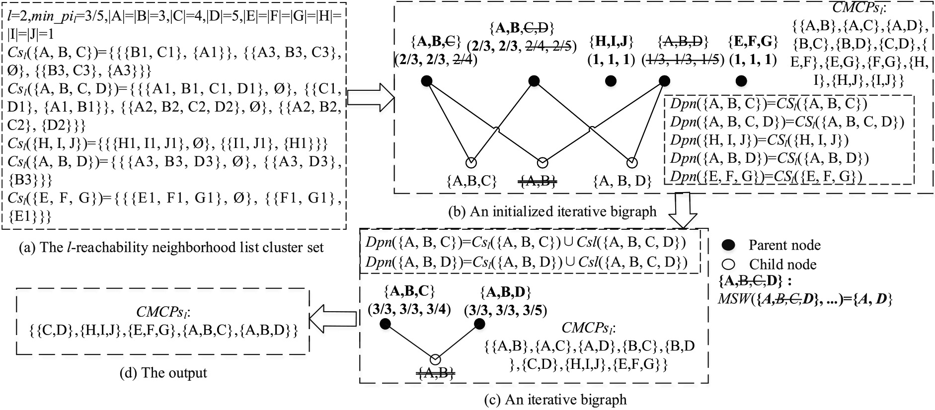

Thus, an example for candidate maximal co-location pattern (or candidate maximal $l$ -reachability co-location pattern) mining on iterative bi-graphs is proposed, as shown in Fig. 4. An $l$ -reachability neighborhood list cluster set is given in Fig. 4a. Figure 4b shows an example of initialized iterative bi-graphs where the parent nodes come from the cluster labels. The child node {A, B} is removed for either $\mid\{\rm{A,B}\}\mid\leqslant 2$ or MSW ({A, B, C}, Dpn ({A, B, C})) $=$ {A, B}. Figure 4c shows an end example of iterations for which there are no child nodes.

[h] : The Iterative Bigraphs ( $I B$ )[1] $Cs_{l}$ , keys, $l$ , $\min\_pi_{l}$ . $\textit{CMCPs}_{l}$ . $k_{0}\in\textit{keys}$ $I B$ . $\textit{creat\_parent}(k_{0})$ //Create parent nodes. $k_{1}\in\textit{keys}$ $\mid k_{0}\cap k_{1}\mid\geqslant 3$ $I B$ . $\textit{create\_child}(IB,k_{0}\cap k_{1})$ //Create child nodes. $p\in IB$ .parents $\textit{MSW}=\textit{msw}(p,\min\_pi_{l})$ //Definition 13. $\textit{update\_cmcp}(\textit{CMCPs}_{l},\textit{MSW})$ //Lemma 6. $c\in IB.\textit{node\_children}(p)$ $c\subseteq\textit{MSW}$ $I B$ . $\textit{remove\_child}(c)$ //Pruning strategy. $I B$ .children $\textit{keys}=IB$ .children //Update child nodes as parent nodes. $IB(Cs_{l},\textit{keys},l,\min\_pi_{l})$ //Recursive algorithm.

To summarize, see Algorithm 4 for details. Algorithm 4 tends to iteratively find candidate maximal $l$ -reachability co-location patterns from iterative bi-graphs. The steps from Step 4 to Step 4 generate child nodes according to parent nodes. The steps from Step 4 to Step 4 check parent nodes (i.e., candidate maximal $l$ -reachability co-location patterns) and remove passed child nodes. The steps from Step 4 to Step 4 start new iterations until all candidate maximal $l$ -reachability co-location patterns have been found.

In Algorithm 4, iterative bi-graphs are initialized by Step 4 to Step 4 and cost $O(n^{2})$ , where $n$ represents the size of the $l$ -reachability neighborhood list cluster set. Since the $l$ -reachability neighborhood lists are generated from instances one by one, $n$ cannot be larger than the size of the instance set $I$ . Each parent node is checked in steps from Step 4 to Step 4. Meanwhile, some candidate maximal $l$ -reachability co-location patterns are detected. This sub-process costs $O(n^{3})$ . Steps from Step 4 to Step 4 are used to iteratively find all candidate maximal $l$ -reachability co-location patterns. Since the depth of the iterations is only related to the intersection sets, the size-independent schema is better than a size-wise method.

4.3 A binary-search approach

Once candidate maximal $l$ -reachability co-location patterns have been generated, maximal $l$ -reachability co-location patterns can be detected. However, it is time-consuming to check the $l$ -reachability table instance for each candidate maximal $l$ -reachability co-location pattern by checking the reachability of pairwise instances in each star $l$ -reachability neighborhood instance. Note that the $\lfloor l/2\rfloor$ -reachability neighborhood list is an $l$ -reachability clique according to Lemma 3, and $l$ -reachability cliques in the star $l$ -reachability neighborhood instance of a candidate maximal $l$ -reachability co-location pattern can be checked in a partial-test way.

Inspection-free $l$ -reachability clique. Assume that we are given $S_{l}(p)$ (a star $l$ -reachability table instance of a pattern $p$ ). For a star $l$ -reachability neighborhood instance $\{s_{0},s_{1}\}\in S_{l}(p)$ , $\{s_{0},s_{1}\}$ can be updated as $\{C_{l},(s_{0}\cup s_{1})-C_{l}\}$ if there exists an $l$ -reachability clique $C_{l}$ that makes $s_{0}\subseteq C_{l}$ . Obviously, initial $l$ -reachability cliques can be collected from $\lfloor l/2\rfloor$ -reachability neighborhood lists according to Lemma 3.

.

Given $S_{2}$ ({A, B, C, D}) $=$ {{{A1, B1, C1, D1}, ø}, {{C1, D1}, {A1, B1}}, {{A2, B2, C2, D2}, ø}, {{A2, B2, C2}, {D2}}}. Since both {A1, B1, C1, D1} and {A2, B2, C2, D2} are 2-reachability cliques, $S_{2}$ ({A, B, C, D}) $=$ {{{A1, B1, C1, D1}, ø}, {{A2, B2, C2, D2}, ø}} because {{A2, B2, C2}, {D2}} has been updated as {{A2, B2, C2, D2}, ø}.

Partial-test of $l$ -reachability instance. Certainly, the corresponding pattern of any $l$ -reachability instance has no duplicate feature according to Definition 3. Consider a star $l$ -reachability neighborhood instance such as $s=\{s_{0},s_{1}\}$ , where $s_{0}$ is an $l$ -reachability clique. For any instance pair $i_{u}$ and $i_{v}$ ( $i_{u}\in s_{0}\wedge i_{v}\in s_{1}$ ), if both $i_{u}$ are not in the $l$ -reachability neighborhood list of $i_{v}$ , and $i_{v}$ is not in the $l$ -reachability neighborhood list of $i_{u}$ (i.e., $(\not\exists s^{\prime}_{0}\in N_{l}(i_{u}))(i_{v}\in s^{\prime}_{0})\wedge(% \not\exists s^{\prime}_{1}\in N_{l}(i_{v}))(i_{u}\in s^{\prime}_{1})$ ), $s$ can be neglected because it cannot be an $l$ -reachability instance. In contrast, $s$ can be accepted as an $l$ -reachability instance unless $(\forall i_{u}\in s_{0})(\forall i_{v}\in s_{1})((\exists s^{\prime}_{0}\in N_% {l}(i_{u}))(i_{v}\in s^{\prime}_{0})\vee(\exists s^{\prime}_{1}\in N_{l}(i_{v}% ))(i_{u}\in s^{\prime}_{1}))$ according to Definition 3.

.

Assume that {{C1, D1}, {A1, B1}} is a star 2-reachability neighborhood instance of {A, B, C, D}. If A1 does not appear in $N_{2}$ (C1) and C1 does not appear in $N_{2}$ (A1), {{C1, D1}, {A1, B1}} can be neglected for {A, B, C, D}.

Once a candidate maximal $l$ -reachability co-location pattern $p$ has been refused, a binary search method is proposed to find maximal $l$ -reachability co-location patterns whose true superset is $p$ rather than using a size-wise approach.

(Binary-subset).

We are given two patterns $p$ and $p^{\prime}(p^{\prime}\subseteq p\subseteq F)$ . The binary subset between $p$ and $p^{\prime}$ (denoted $BS(p,p^{\prime})$ ) is a set that comprises all size- $\lfloor(\mid p\mid+\mid p^{\prime}\mid)/2\rfloor$ subsets of $p$ . Namely,

$\displaystyle BS(p,p^{\prime})=\{b\mid p^{\prime}\subseteq b\subseteq p,\mid b% \mid=\lfloor(\mid p\mid+\mid p^{\prime}\mid)/2\rfloor\}$ (13)

.

$B S$ ({A, B}, {A, B, C, D, E}) $=$ {{A, B, C}, {A, B, D}, {A, B, E}}.

(Acceptance of $\textit{MCPs}_{l}$ ).

Assume that we are given an $l$ -reachability threshold $\min\_pi_{l}$ and a candidate maximal $l$ -reachability co-location pattern set $\textit{CMCPs}_{l}$ . A maximal $l$ -reachability co-location pattern set $\textit{MCPs}_{l}=\cup_{p\in\textit{CMCPs}_{l}}\{p^{\prime}\mid p^{\prime}% \subseteq p,PI_{l}(p^{\prime})\geqslant\min\_pi_{l},p^{\prime}\in BS(p,p^{% \prime})\}$ .

Proof..

Assume that we are given an $l$ -reachability threshold $\min\_pi_{l}$ and candidate maximal $l$ -reachability co-location pattern set $\textit{CMCPs}_{l}$ . Let $m p$ be a maximal $l$ -reachability co-location pattern. Let $x$ be a candidate maximal $l$ -reachability co-location pattern and be a superset of $m p$ , namely, $x\in\textit{CMCPs}_{l}\wedge mp\subseteq x$ . Since $\textit{MCPs}_{l}=\max(\cup_{p\in\textit{CMCPs}_{l}}\{p^{\prime}\mid p^{\prime% }\subseteq p,PI_{l}(p^{\prime})\geqslant\min\_pi_{l},p^{\prime}\in BS(p,p^{% \prime})\})$ , maximal subset winners between $x$ and $\o$ have been found. In other words, $m p$ must be one of $MSW(x,\o)$ . In other words, $m p$ must be in $\textit{MCPs}_{l}$ . Furthermore, it is assumed that there exists a pattern $x^{\prime}$ in $\cup_{p\in\textit{CMCPs}_{l}}\{p^{\prime}\mid p^{\prime}\subseteq p,PI_{l}(p^{% \prime})\geqslant\textit{min}\_pi_{l},p^{\prime}\in BS(p,p^{\prime})\}$ that is not a maximal $l$ -reachability co-location pattern. Namely, $x^{\prime}\in\cup_{p\in\textit{CMCPs}_{l}}\{p^{\prime}\mid p^{\prime}\subseteq p% ,PI_{l}(p^{\prime})\geqslant\textit{min}\_pi_{l},p^{\prime}\in BS(p,p^{\prime}% )\}\wedge x^{\prime}\notin\textit{MCPs}_{l}$ . In other words, there exist two possibilities. First, $x^{\prime}$ is not an $l$ -reachability co-location pattern, because $\max(s)$ returns the maximal pattern of $s$ , namely, $PI_{l}(x^{\prime})<\textit{min}\_pi_{l}$ . It contradicts the $\cup_{p\in\textit{CMCPs}_{l}}\{p^{\prime}\mid p^{\prime}\subseteq p,PI_{l}(p^{% \prime})\geqslant\textit{min}\_pi_{l},p^{\prime}\in BS(p,p^{\prime})\}$ . Second, there exists a true maximal $l$ -reachability co-location pattern $mp^{\prime}$ ( $x^{\prime}\subset mp^{\prime}\in\textit{MCPs}_{l}$ ). Since $mp^{\prime}\in\cup_{p\in\textit{CMCPs}_{l}}\{p^{\prime}\mid p^{\prime}% \subseteq p,PI_{l}(p^{\prime})\geqslant\textit{min}\_pi_{l},p^{\prime}\in BS(p% ,p^{\prime})\}$ has been proved, $mp^{\prime}=x^{\prime}$ , which contradicts the hypothesis. In other words, the lemma is proved. ∎

.

We are given a candidate maximal $l$ -reachability co-location pattern {A, B, C, D, E, F, G, H} and one of its subsets {A, C, D, G}, which is also a maximal $l$ -reachability co-location pattern. To obtain {A, C, D, G}, the search path (traversal sequence) in a binary-search approach can be {A, B, C, D, E, F, G, H} $\longrightarrow$ {A, B, C, D, G} ( $\lfloor(3+7)/2\rfloor=5$ ) $\longrightarrow$ {A, C, D} ( $\lfloor(3+4)/2\rfloor=3$ ) $\longrightarrow$ {A, C, D, G} ( $\lfloor(4+4)/2\rfloor=4$ ) instead of {A, B, C, D, E, F, G, H} $\longrightarrow$ {A, B, C, D, E, F, G} $\longrightarrow$ {A, B, C, D, E, G} $\longrightarrow$ {A, B, C, D, G} $\longrightarrow$ {A, C, D, G} in an size-wise way. The deletion lines indicate rejection.

Obviously, a binary-subset winner can be checked to determine whether it has appeared in the maximal $l$ -reachability co-location patterns before checking its true prevalence to reduce repetition. The binary search method costs $O(1)$ at best and costs

$\displaystyle O\left(\sum_{i=1}^{\log_{2}{k}}C_{k}^{k^{\prime}}\right)$

on average, where $0\leqslant k^{\prime}\leqslant k$ , and where $k$ represents the size of a candidate maximal $l$ -reachability co-location pattern and $k^{\prime}$ represents the mean size of maximal $l$ -reachability co-location patterns led by the candidate. Because the binary search is $O(\log_{2}k)$ on average, there exist $C_{k}^{\frac{(2^{i}-1)k+2^{i}}{2^{i}}}$ (or $C_{k}^{\frac{k+2^{i}}{2^{i}}}$ ) binary subsets in the $i$ -th time. This finding is obviously better than $O(2^{k})$ (i.e., $O(\sum_{i=1}^{k}C_{k}^{k^{\prime}/2}$ ) for the time complexity in a size-wise approach on average, where $0\leqslant k^{\prime}\leqslant k$ .

4.4 An improved method

Since sparsification strategies, iterative bi-graphs and binary search methods have been proposed, an improved method called the improved method ( $I M$ ) is integrated. Step 3 obtains $\lfloor l/2\rfloor$ -reachability neighborhood lists and $l$ -reachability neighborhood lists in the reversed binary search method. Step 4.4 works on the sparsification strategies. Step 4.4 is Algorithm 4. The steps from Step 4.4 to Step 4.4 check candidate maximal $l$ -reachability co-location patterns in a binary search approach.

: The Improved Method ( $I M$ ))[1] $G=(I,R)$ , $l$ , $\textit{min}\_pi_{l}$ . $\textit{MCPs}_{l}$ . $Ns_{\lfloor l/2\rfloor}$ , $Ns_{l}=\textit{reversed\_binary}(G,l)$ //Lemma 4. $Cs_{l},Ps2=SS(N_{l},N_{\lfloor l/2\rfloor})$ //Sparsification strategies. $\textit{CMCPs}_{l}=IB(Cs_{l},\textit{min}\_pi_{l})$ //Algorithm 4. $\textit{MCPs}_{l}=Ps2$ //Initial $\textit{MCPs}_{l}$ as size-2 $l$ -reachability co-location patterns. $p\in\textit{CMCPs}_{l}$ $S_{l}=\textit{star\_gen}(Cs_{l},p)$ //Definition 9. $\textit{MCPs}_{l}\cup=\textit{check}(S_{l},Ns_{l},Ns_{\lfloor l/2\rfloor})$ //Lemma 8. $\textit{MCPs}_{l}=\max(\textit{MCPs}_{l})$ //Lemma 8.

Since the time complexities of both steps from Step 4.4 to Step 4.4 of Algorithm 3 and Algorithm 4 have been analyzed, we only need to analyze the time complexities of steps from Step 4.4 to Step 4.4 for Algorithm 4.4. Although Step 4.4 is an NP-hard problem, it is acceptable that the candidate maximal $l$ -reachability co-location pattern $p$ is approximated to the true maximal $l$ -reachability co-location pattern. Interestingly, Algorithm 4.4 is also workable even if $l=$ 1 (i.e., it is workable for classical co-location pattern mining).

5. Experiments

In this section, both the baseline method and the improved method in this paper are evaluated with synthetic and real data sets distributed as shown in Fig. 5. The coordinates of both graphs are accurate in meters. Table 1 shows the abbreviations. In addition, the experimental platform is based on a personal computer with an Intel (R) Core (TM) i7-8700 CPU running 3.20 GHz and 3.19 GHz in addition to 32 GB RAM following Windows10 64-bit OS.

Table 1
The abbreviation table for experiments

Abbreviation	Full name
$d$	A distance threshold given by users
$l$	A step length given by users
$\min\_pi_{l}$	An $l$ -reachability prevalence threshold given by users
$B M$	The base-line method (Algorithm 3)
$S S$	The sparsification strategies
$I B$	The iterative bi-graphs method (Algorithm 4)
$B S$	The binary-search way
$I M$	The improved method (Algorithm 4.4)
$\textit{CPs}\_l$	An corresponding pattern set for some instances
$Cs_{l}$	The $l$ -reachability neighborhood list cluster set
$Ns_{l}$	The $l$ -reachability neighborhood list set
$\textit{ins}^{\prime}_{l}$	The $l$ -reachability instance set (i.e., $\cup_{p\rm{IsAPatternSet}}\textit{ins}_{l}(p)$ )
$\textit{MCs}_{l}$	The maximal $l$ -reachability clique set
$\textit{CMCPs}_{l}$	The candidate maximal $l$ -reachability co-location pattern set
$\textit{MCPs}_{l}$	The $l$ -reachability co-location pattern set
count	The count of elements of a set
Size (or mean size)	The length of an element (or the mean length of elements)

Figure 5.

Spatial instance distributions of experimental data sets.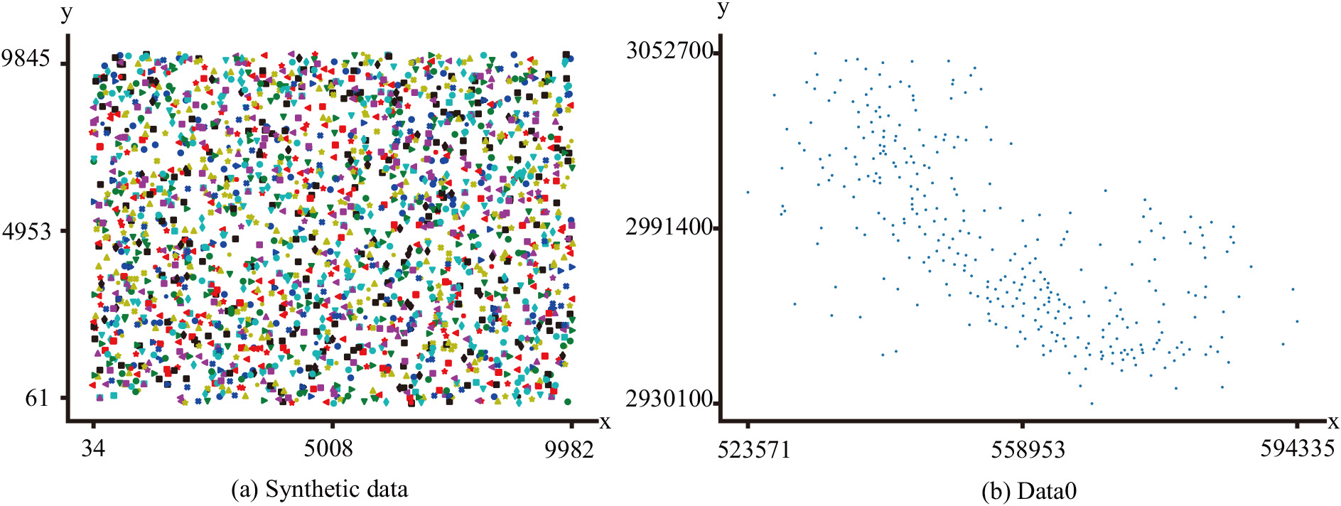

5.1 Data sets

5.1.1 Synthetic data sets

The synthetic data sets called synthetic data (i.e., Fig. 5a) tend to synthesize spatial feature instances that contain 100 expected maximal patterns. The 100 patterns are called expected positive examples of patterns ( $P$ for short).

5.1.2 Real data sets

The real data sets called Data0 (i.e., Fig. 5b) present a rare plant spatial distribution in the Three Parallel Rivers Yunnan Protected Areas [28]. All 337 rare plants classified into 31 features were evenly and sparsely distributed. The distance threshold $d=$ 2500 m (meters) and the step length threshold $l=$ 3 are suggested to be optimal parameters for Data0 by repeated tests in the $l$ -reachability co-location pattern mining model.

Figure 6.

The test result on synthetic data.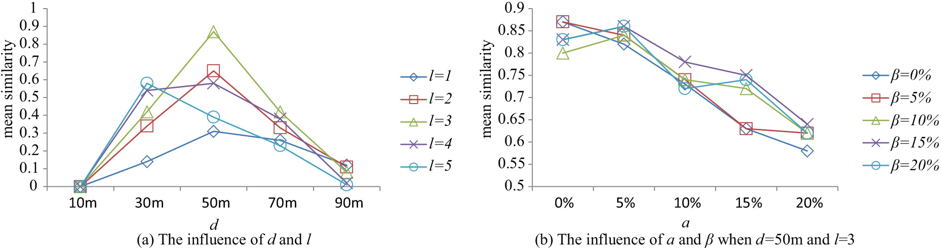

The coordinates of the data sets are accurate to meters. The suggested prevalence threshold $\min\_pi_{l}$ is 0.1 for either synthetic data or Data0.

Figure 7.

The $l$ test result shown on Data0.

Figure 8.

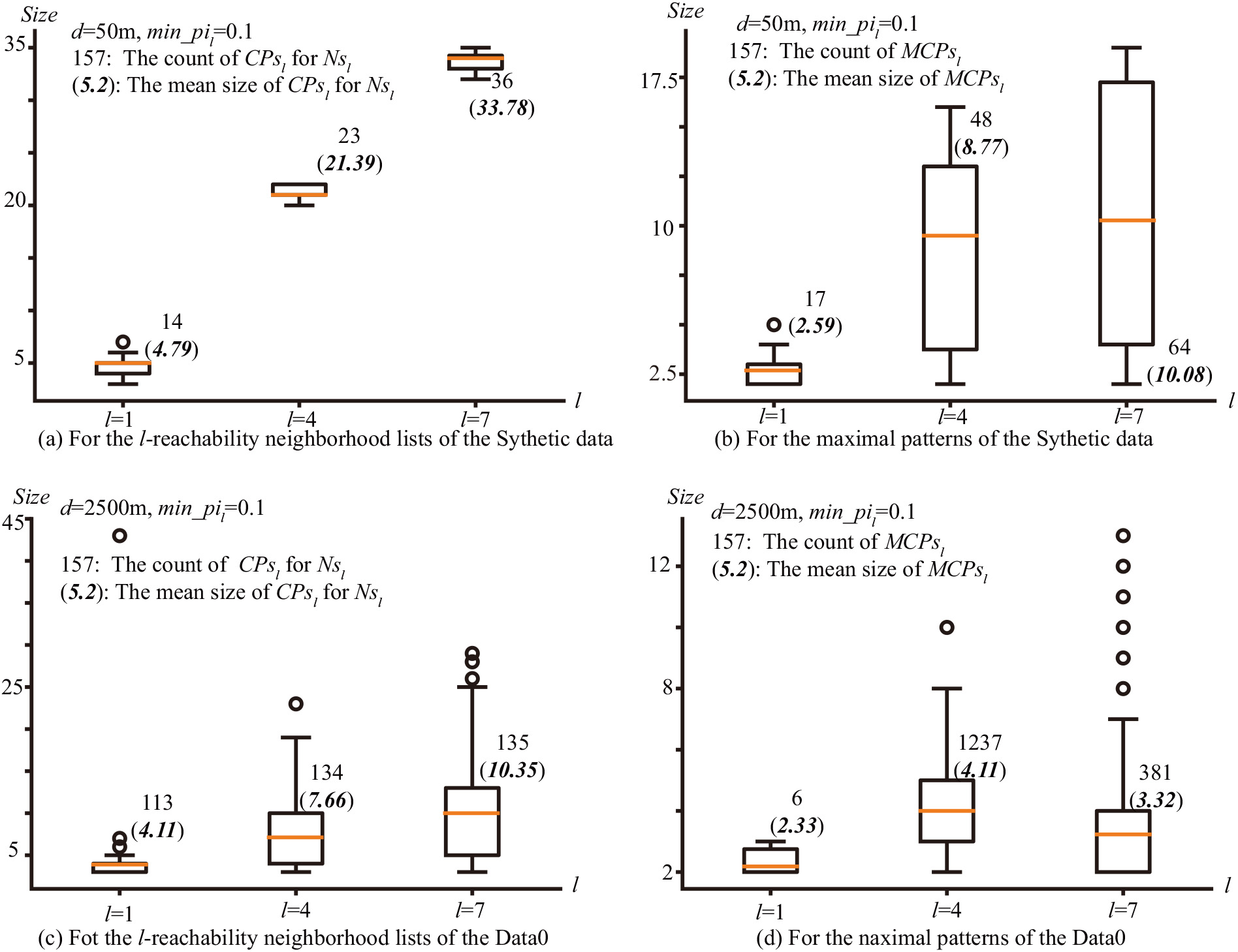
The comparison of the intermediate results (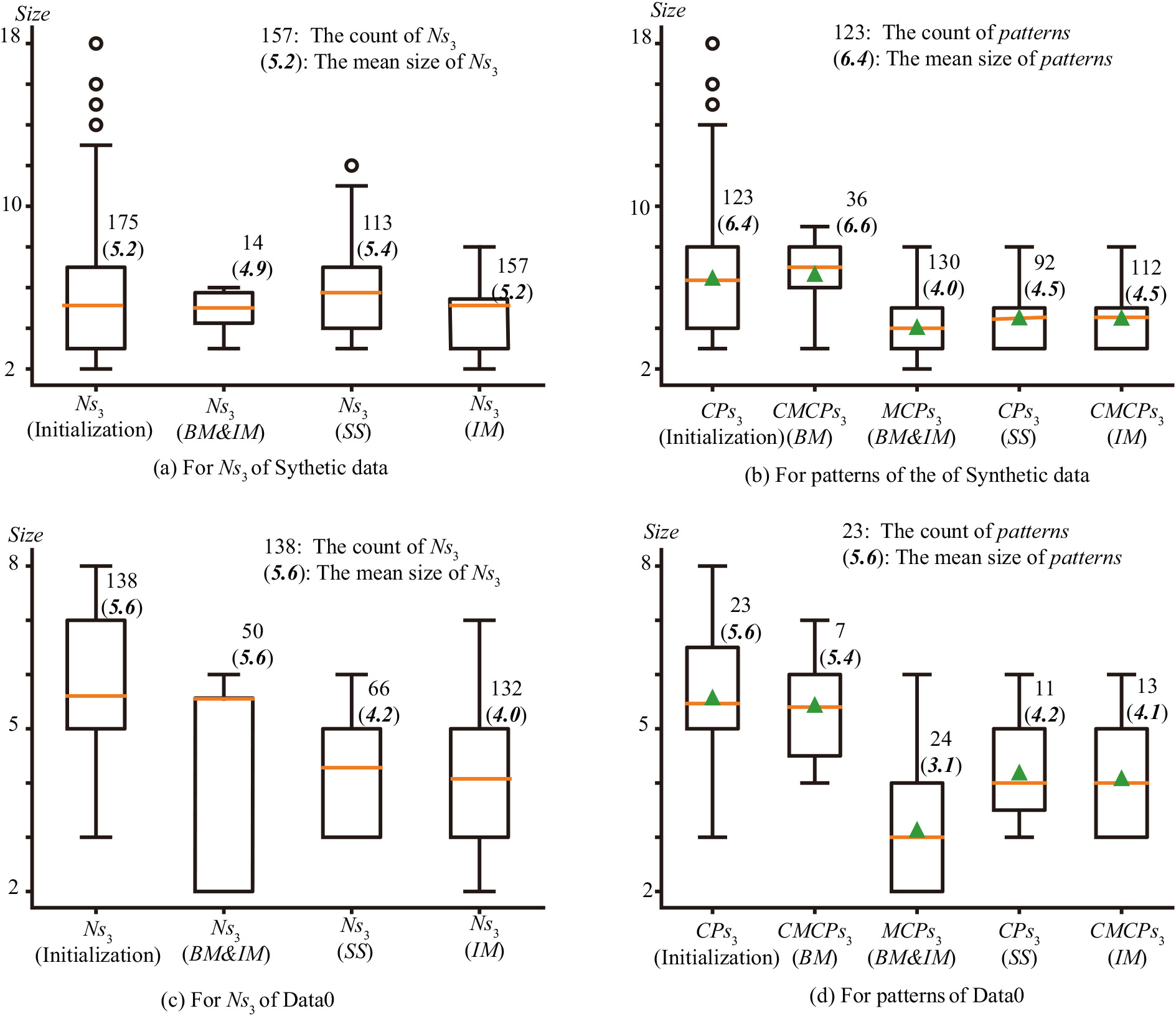 $\min\_pi_{l}=0.1$ ).

Figure 9.

The comparison of checked objects (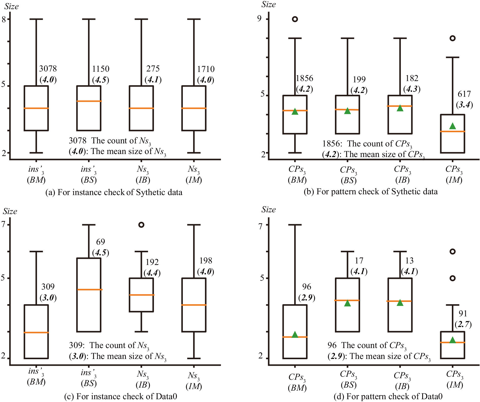 $\min\_pi_{l}=0.1$ ).

Figure 10.

The execution times on synthetic data.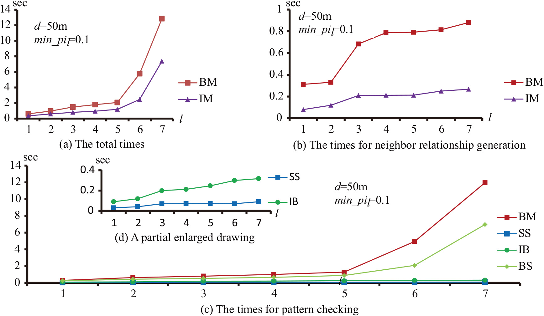

5.2 Experimental results and analysis

5.2.1 Mean similarity

The mean similarity between expected patterns (i.e., $P$ ) and the discovered maximal patterns (denoted $D P$ ) is defined as

$\displaystyle\frac{\sum_{c\in P}\max_{c^{\prime}\in DP}\max\{0,\mid c\cap c^{% \prime}\mid-\mid c^{\prime}-c\mid\}/\mid c\mid}{\mid P\mid}$

The closer the mean similarity is to 1, the better the performance of our maximal $l$ -reachability co-location pattern model. Since the expected maximal patterns are difficult to define in real data sets, they are tested on synthetic data.

Figure 6a shows the mean similarity of our $l$ -reachability co-location pattern model in comparison of different distance thresholds and step length thresholds on the synthetic dataset. Certainly, the 1-reachability co-location pattern model is equal to the classical co-location pattern model. This finding reveals that an optimal step length $l$ can improve the mean similarity of the mining results when a distance threshold $d$ is less than the optimal distance threshold. For example, the mean similarity on $l=3$ is larger than that on $l=1$ when $d=30$ m. In contrast, a multiple $l$ can lead to a lower mean similarity than the same multiple $d$ . Furthermore, an increase in $l$ at the same growth rate will make the mean similarity more robust than an increase in $d$ when the growth makes $d$ larger than the optimal distance threshold. For example, the mean similarity at $l=2$ and $d=30$ m is closer to the highest mean similarity than that at $l=1$ and $d=70$ m when the initialization is $l=1$ and $d=10$ m. Importantly, the highest mean similarity of the classical co-location pattern model ( $l=1$ ) is 0.31 when one of the $l$ -reachability co-location pattern models is 0.87 when the growth gradient of $d$ is 20 m. In other words, the $l$ -reachability co-location pattern model can improve the mining results.

Figure 6b shows the influence of noise instances (its ratio denotes $\beta$ ) and missing instances (its ratio denotes $\alpha$ ). The higher the $\beta$ when $\alpha=$ 0%, the lower the mean similarity, so is the $\alpha$ when $\beta=$ 0%. If the both coexist, the can offset each other to mean similarity.

5.2.2 Sensibility

The sensibility is used to test the effect of $l$ on the $l$ -reachability co-location patterns. It will be shown in boxplots such as Fig. 7. A boxplot (or box-and-whisker plot) shows the distribution of quantitative data in a way that facilitates comparisons between variables or across levels of a categorical variable. The boxplot shows the quartiles of the dataset, while the whiskers extend to show the remainder of the distribution, except for points that are determined to be outliers (i.e., small circles in the boxplot) using a method that is a function of the interquartile range. In Fig. 7, the boxplots show that more maximal $l$ -reachability co-location patterns with larger sizes are discovered with the growth of the step length $l$ . For example, the largest size of the maximal 7-reachability co-location patterns becomes 13, while one of the maximal 4-reachability co-location patterns becomes 10 when $d=$ 2500 m on Data0. In other words, the results are sensitive to $l$ . A larger $l$ can help users to discover more interesting patterns.

5.2.3 Effectiveness

The effectiveness is used to evaluate our improved $l$ -reachability co-location pattern mining model in comparison to the baseline method.

The most time-consuming part of $l$ -reachability co-location pattern mining is the $l$ -reachability clique check. That is, the fewer $l$ -reachability cliques the better. Moreover, the shorter the size of each $l$ -reachability clique, the better. Since an $l$ -reachability clique comes from an $l$ -reachability neighborhood list, the fewer $l$ -reachability neighborhood lists the better. Similarly, the shorter the size of the $l$ -reachability list of each instance, the better. Thus, boxplots are used to show $l$ -reachability clique sizes (or $l$ -reachability neighborhood list sizes) and their corresponding patterns. Since the count of subsets is $2^{k}$ for a size- $k$ $l$ -reachability clique or $l$ -reachability neighborhood list, the mean sizes and medians (green triangles for patterns) are more worthy of attention in the comparison of counts.

Therefore, Fig. 8 shows the distributions of procedure results. This figure reveals that the mean sizes of candidate maximal $l$ -reachability co-location patterns generated by the improved method are shorter than those from the baseline method. That is, fewer costs are needed with the improved method than with the baseline method. Figure 9 corroborates this finding in detail.

Figure 11.

The execution times on Data0.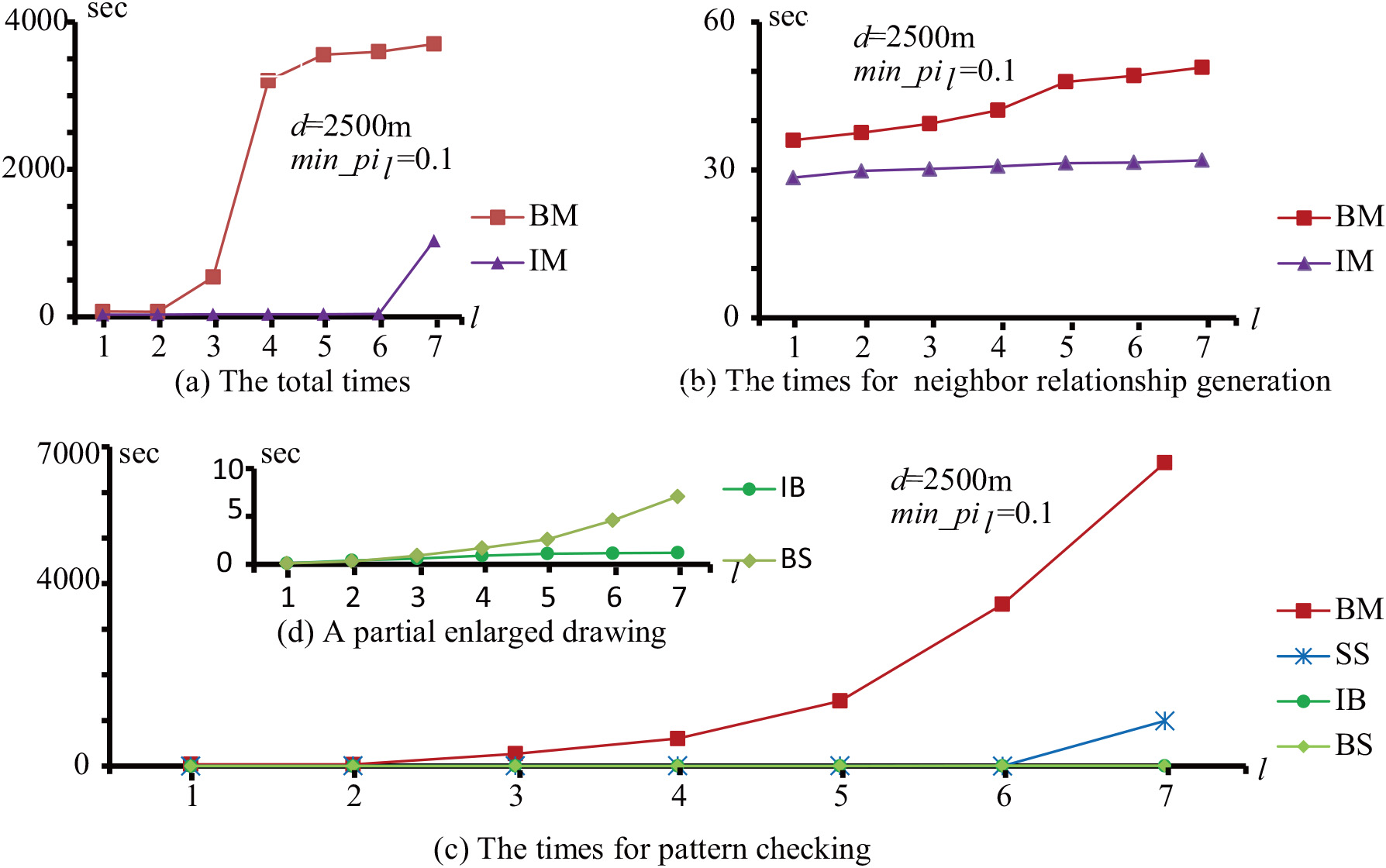

5.2.4 Efficiency

The efficiency of the improved method is evaluated in comparison to the baseline method by the execution times of the algorithms. Figures 10 and 11 show that the improved method is highly efficient when a distance threshold $d$ , a step length threshold $l$ and an $l$ -reachability prevalence threshold $\min\_pi_{l}$ are given in comparison with the baseline method.

In other words, our $l$ -reachability co-location pattern model works well and reflects the indirect correlation of instances across mediation instances. Meanwhile, the improved method for maximal $l$ -reachability co-location pattern mining is more effective than the baseline method.

6. Conclusions

The $l$ -reachability clique has been introduced as an extension of the clique and star relationships in this paper. Furthermore, the $l$ -reachability co-location pattern based on the $l$ -reachability clique has extended the classical co-location pattern and the sub-prevalent pattern. Since the average size of $l$ -reachability co-location patterns tends to be longer than co-location patterns and sub-prevalent patterns, maximal $l$ -reachability co-location pattern mining has been researched. Sparsification strategies are workable to shorten star neighborhood lists in $l$ -reachability neighbor relationship graphs. Furthermore, iterative bi-graphs can lead to a size-independent way of generating candidate maximal $l$ -reachability co-location patterns. With the help of the $\lfloor l/2\rfloor$ -reachability neighborhood list, our binary-search method is more efficient in checking maximal $l$ -reachability co-location patterns with the partial test of $l$ -reachability cliques.

In a co-location pattern, a feature tends to be more important if the feature’s instances always have a high closeness centrality in its co-location instances. The closeness centrality of each instance in an $l$ -reachability clique can be generally different when $l$ is larger than 1. Along this line, the importance of each feature in $l$ -reachability co-location patterns can be measured rather than only following a test method with changes in the participation ratios. Furthermore, the importance of a feature changes as some other spatial features are added. The reason for these changes must be interesting because the changes imply correlation or cooccurrence of spatial features. Thus, all of the above will be followed.

Footnotes

Acknowledgments

This paper is supported by the National Natural Science Foundation of China (No. 61966036, 61662086, 62066023), the Yunnan Province Scientific Innovation Team Project (No. 2018HC019), and the Scientific Research Project of Kunming University (No. XJZZ1706).

Conflict of interest

The authors declare that they have no conflict of interest.

References

Gao

Lin

Qian

and Lin

, Spatial pattern analysis reveals multiple sources of organophosphorus flame retardants in coastal waters, Journal of Hazardous Materials 417 (2021), 125882. doi: 10.1016/J.JHAZMAT.2021.125882.

Adilmagambetov

Jabbar

M.S.M.

Zaïane

O.R.

Osornio-Vargas

and Wine

, On discovering co-location patterns in datasets: A case study of pollutants and child cancers, GeoInformatica 2016 20:4 20 (2016), 651–692. doi: 10.1007/S10707-016-0254-1.

Moosavi

Samavatian

M.H.

Nandi

Parthasarathy

and Ramnath

, Short and Long-term Pattern Dis-covery Over Large-Scale Geo-Spatiotemporal Data, in: Proceedings of the 25th ACM SIGKDD International Conference on Knowledge Discovery and Data Mining, Vol. 19, 2019. ISBN 9781450362016. doi: 10.1145/3292500.

Wang

Bao

and Zhou

, Redundancy reduction for prevalent co-location patterns, IEEE Transactions on Knowledge and Data Engineering 30 (2018), 142–155. doi: 10.1109/TKDE.2017.2759110.

Chan

H.K.H.

Long

Yan

and Wong

R.C.W.

, Fraction-score: A new support measure for co-location pattern mining, in: Proceedings – International Conference on Data Engineering, 2019-April, 2019, pp. 1514–1525. ISBN 9781538674741. doi: 10.1109/ICDE.2019.00136.

Huang

Pei

and Xiong

, Mining co-location patterns with rare events from spatial data sets, GeoInformatica 10 (2006), 239–260. doi: 10.1007/S10707-006-9827-8.

Yao

Chen

Wen

Peng

Yang

Chi

Wang

and Yu

, A spatial co-location mining algorithm that includes adaptive proximity improvements and distant instance references, https://doi.org/10.1080/13658816.2018.1431839 32 (2018), 980–1005. doi: 10.1080/13658816.2018.1431839.

Huang

Shekhar

and Xiong

, Discovering colocation patterns from spatial data sets: A general approach, IEEE Transactions on Knowledge and Data Engineering 16 (2004), 1472–1485. doi: 10.1109/TKDE.2004.90.

Zala

M.R.L.

Mehta

M.B.B.

and Zala

M.M.R.

, A survey on spatial co-location patterns discovery from spatial datasets, International Journal of Computer Trends and Technology 7 (2014), 137–142. doi: 10.14445/22312803/IJCTT-V7P140.

10.

Yoo

J.S.

and Shekhar

, A joinless approach for mining spatial colocation patterns, IEEE Transactions on Knowledge and Data Engineering 18 (2006), 1323–1337. doi: 10.1109/TKDE.2006.150.

11.

and Shekhar

, Local Co-location Pattern Detection: A Summary of Results, DROPS-IDN/9338 114 (2018). ISBN 9783959770835. doi: 10.4230/LIPICS.GISCIENCE.2018.10.

12.

Wang

Bao

Zhou

and Chen

, Maximal sub-prevalent co-location patterns and efficient mining algorithms, Lecture Notes in Computer Science (Including Subseries Lecture Notes in Artificial Intelligence and Lecture Notes in Bioinformatics) 10569 LNCS (2017), 199–214. ISBN 9783319687827. doi: 10.1007/978-3-319-68783-4_14.

13.

Guo

, The Research into the World Heritage Value and Tourism Development of Dike-Pond Agriculture in the Pearl River Delta, Tourism and Hospitality Development Between China and EU, 2015, 111–127. doi: 10.1007/978-3-642-35910-1_9.

14.

Bao

Wang

and Zhao

, Mining top-k-size maximal co-location patterns, in: IEEE CITS 2016 – 2016 International Conference on Computer, Information and Telecommunication Systems, 2016. ISBN 9781509034406. doi: 10.1109/CITS.2016.7546421.

15.

Shekhar

and Huang

, Discovering Spatial Co-location Patterns: A Summary of Results, Lecture Notes in Computer Science (including subseries Lecture Notes in Artificial Intelligence and Lecture Notes in Bioinformatics) 2121 (2001), 236–256. ISBN 9783540423010. doi: 10.1007/3-540-47724-1-13.

16.

Wang

and Duan

, Mining Maximal Dynamic Spatial Co-Location Patterns, IEEE Transactions on Neural Networks and Learning Systems 32 (2018), 1026–1036. doi: 10.1109/TNNLS.2020.2979875.

17.

Wang

Ying

Kong

and Tang

, Research of mining algorithms for uncertain spatio-temporal co-occurrence pattern, in: 2017 9th International Conference on Knowledge and Smart Technology (KST), 2017, pp. 12–17. doi: 10.1109/KST.2017.7886070.

18.

Yin

Zheng

and Cao

, USpan: An efficient algorithm for mining high utility sequential patterns, ACM, 2012.

19.

Yao

Wang

Peng

and Chi

, An adaptive maximal co-location mining algorithm, International Geoscience and Remote Sensing Symposium (IGARSS) 2017-July (2017), 5551–5554. ISBN 9781509049516. doi: 10.1109/IGARSS.2017.8128262.

20.

Qian

Chiew

Huang

and Ma

, Discovery of regional co-location patterns with k-nearest neighbor graph, Lecture Notes in Computer Science (Including Subseries Lecture Notes in Artificial Intelligence and Lecture Notes in Bioinformatics) 7818 LNAI (2013), 174–186. ISBN 9783642374524. doi: 10.1007/978-3-642-37453-1_15.

21.

Yao

Chen

Peng

and Chi

, A co-location pattern-mining algorithm with a density-weighted distance thresholding consideration, Information Sciences 396 (2017), 144–161. doi: 10.1016/J.INS.2017.02.040.

22.

Kumar

G.K.

Kavati

Rao

K.S.

and Cheruku

, Spatial co-location pattern mining using delaunay triangulation, Advances in Intelligent Systems and Computing 705 (2018), 95–102. ISBN 9789811085680. doi: 10.1007/978-981-10-8569-7_10.

23.

Bayat

Nasseri

and Zahraie

, Identification of long-term annual pattern of meteorological drought based on spatiotemporal methods: Evaluation of different geostatistical approaches, Natural Hazards 76 (2015), 515–541. doi: 10.1007/S11069-014-1499-3.

24.

Huang

Zhang

and Zhang

, On the relationships between clustering and spatial co-location pattern mining, https://dx-doi-org.web.bisu.edu.cn/10.1142/S0218213008003777 17 (2011), 55–70. doi: 10.1142/S0218213008003777.

25.

Bao

and Wang

, A clique-based approach for co-location pattern mining, Information Sciences 490 (2019), 244–264. doi: 10.1016/J.INS.2019.03.072.

26.

Yang

Wang

and Wang

, A MapReduce approach for spatial co-location pattern mining via ordered-clique-growth, Distributed and Parallel Databases 38 (2019), 531–560. doi: 10.1007/S10619-019-07278-7.

27.

Tran

Wang

and Zhou

, Mining Spatial Co-Location Patterns Based on Overlap Maximal Clique Partitioning, in: 2019 20th IEEE International Conference on Mobile Data Management (MDM), 2019.

28.

Wang

and Chen

, Finding probabilistic prevalent colocations in spatially uncertain data sets, IEEE Transactions on Knowledge and Data Engineering 25 (2013), 790–804. doi: 10.1109/TKDE.2011.256.

29.

Berry

and Pogorelcnik

, A simple algorithm to generate the minimal separators and the maximal cliques of a chordal graph, Information Processing Letters 111 (2011), 508–511. doi: 10.1016/J.IPL.2011.02.013.

30.

Rinzivillo

and Turini

, Extracting spatial association rules from spatial transactions, GIS: Proceedings of the ACM International Symposium on Advances in Geographic Information Systems, 2005, 79–86. doi: 10.1145/1097064.1097077.

31.

Eppstein

Löffler

and Strash

, Listing All Maximal Cliques in Sparse Graphs in Near-optimal Time, Lecture Notes in Computer Science (including subseries Lecture Notes in Artificial Intelligence and Lecture Notes in Bioinformatics), 6506 LNCS, 403–414. ISBN 3642175163. doi: 10.1007/978-3-642-17517-6_36.

32.

Han

Pei

Yin

and Mao

, Mining frequent patterns without candidate generation: A frequent-pattern tree approach, Data Mining and Knowledge Discovery 8 (2004), 53–87. doi: 10.1023/B:DAMI.0000005258.31418.83.

33.

Yoo

J.S.

and Bow

, Mining top-k closed co-location patterns, in: ICSDM 2011 – Proceedings 2011 IEEE International Conference on Spatial Data Mining and Geographical Knowledge Services, 2011, pp. 100–105. ISBN 9781424483495. doi: 10.1109/ICSDM.2011.5969013.

34.

Yao

Peng

Yang

and Chi

, A fast space-saving algorithm for maximal co-location pattern mining, Expert Systems with Applications 63 (2016), 310–323. doi: 10.1016/J.ESWA.2016.07.007.

35.

Aini

and Salehipour

, Speeding up the Floyd-Warshall algorithm for the cycled shortest path problem, Applied Mathematics Letters 25 (2012), 1–5. doi: 10.1016/J.AML.2011.06.008.

Efficiently mining maximal l -reachability co-location patterns from spatial data sets

Abstract

Keywords

1. Introduction

1.1 Context

1.3 Roadmap

3. Maximal l -reachability co-location pattern

3.1 l -reachability co-location pattern

( l -reachability neighborhood list).

( l -reachability clique).

(Nestedness of l -reachability cliques).

Proof..

.

( l -reachability instance).

.

( l -reachability participation ratio).

.

( l -reachability participation index).

( l -reachability co-location pattern).

.

(Anti-monotonicity of P ⁢ R l ⁢ ( p , f i ) and P ⁢ I l ⁢ ( p ) ).

Proof..

(Maximal l -reachability co-location pattern).

.

4.1 A natural l -reachability clique

(A natural l -reachability clique).

Proof..

.

(Reversed binary-search of N l ⁢ ( i u ) ).

Proof..

( l -reachability neighborhood list cluster).

(Star l -reachability neighborhood instance).

.

(Upper participation ratio).

(Upper participation index).

.

(Anti-monotonicity of 𝑈𝑃𝑅 l ⁢ ( p , f i ) and 𝑈𝑃𝐼 l ⁢ ( p ) ).

Proof..

(Candidate maximal l -reachability co-location pattern).

(Maximal subset winner).

.

(Suggestion for 𝐶𝑀𝐶𝑃𝑠 l ).

Proof..

(Iterative bi-graphs).

.

(The perfect matching for 𝐶𝑀𝐶𝑃𝑠 l mining).

Proof..

.

.

(Binary-subset).

.

(Acceptance of 𝑀𝐶𝑃𝑠 l ).

Proof..

.

5. Experiments

Table 1 The abbreviation table for experiments

5.1.1 Synthetic data sets

5.1.2 Real data sets

5.2.1 Mean similarity

5.2.2 Sensibility

5.2.3 Effectiveness

6. Conclusions

Footnotes

Acknowledgments

Conflict of interest

References

3. Maximal $l$ -reachability co-location pattern

3.1 $l$ -reachability co-location pattern

( $l$ -reachability neighborhood list).

( $l$ -reachability clique).

(Nestedness of $l$ -reachability cliques).

( $l$ -reachability instance).

( $l$ -reachability participation ratio).

( $l$ -reachability participation index).

( $l$ -reachability co-location pattern).

(Anti-monotonicity of $PR_{l}(p,f_{i})$ and $PI_{l}(p)$ ).

(Maximal $l$ -reachability co-location pattern).

4.1 A natural $l$ -reachability clique

(A natural $l$ -reachability clique).

(Reversed binary-search of $N_{l}(i_{u})$ ).

( $l$ -reachability neighborhood list cluster).

(Star $l$ -reachability neighborhood instance).

(Anti-monotonicity of $\textit{UPR}_{l}(p,f_{i})$ and $\textit{UPI}_{l}(p)$ ).

(Candidate maximal $l$ -reachability co-location pattern).

(Suggestion for $\textit{CMCPs}_{l}$ ).

(The perfect matching for $\textit{CMCPs}_{l}$ mining).

(Acceptance of $\textit{MCPs}_{l}$ ).

Table 1
The abbreviation table for experiments