Learning binary codes for fast image retrieval with sparse discriminant analysis and deep autoencoders

Abstract

Image retrieval with relevant feedback on large and high-dimensional image databases is a challenging task. In this paper, we propose an image retrieval method, called BCFIR (Binary Codes for Fast Image Retrieval). BCFIR utilizes sparse discriminant analysis to select the most important original feature set, and solve the small class problem in the relevance feedback. Besides, to increase the retrieval performance on large-scale image databases, in addition to BCFIR mapping real-valued features to short binary codes, it also applies a bagging learning strategy to improve the ability general capabilities of autoencoders. In addition, our proposed method also takes advantage of both labeled and unlabeled samples to improve the retrieval precision. The experimental results on three databases demonstrate that the proposed method obtains competitive precision compared with other state-of-the-art image retrieval methods.

Keywords

Content-based image retrieval (CBIR)sparse discriminant analysis deep autoencoder binary code

1. Introduction

Content-based image retrieval (CBIR) with relevant feedback has been an active area of research over the past decade [6, 16, 37, 45, 46, 48]. Measuring the similarity between two images by Euclidean distance in multi-dimensional space is often ineffective because there exists a semantic gap between the low-level visual features and the high-level semantic concepts of the image. To reduce this semantic gap, the approach is to include classifier machine learning in the retrieval process. In the returned results, this mechanism allows the user to assign positive labels to images that are semantically similar to the query image and also allows the user to assign negative labels to images that are not semantically similar to the query image. These feedback samples are used as the training set for the classifier machine learning technique. Because the number of feedback samples obtained is very small compared to the dimensionality of the feature space of the image data, it is difficult to obtain a good classification learning model. In this situation, people often find ways to reduce the image data dimensionality, which obtains a lower dimensional projection space [22, 24, 29, 39]. In this low-dimensional projection space, machine learning techniques are applied to learn high-level semantic concepts.

Dimensional reduction is one of the most effective techniques for classification machine learning problems on multidimensional data [52, 55]. It is proposed to solve the problem of the “curse of dimensionality” [8], which means that machine learning models cannot perform effectively when dealing with high-dimensional data. Recently, many classification machine learning models have been proposed such as multiple-instance learning [53] and subspace learning. The most well-known projection space learning methods include principal component analysis (PCA) [25] and Linear discriminant analysis (LDA) [13, 40]. PCA learns a projection that can preserve the information of the data, while LDA finds an optimal discriminant projection space such that the ratio of between-class scatters to within-class scatter is maximized. However, if image retrieval relies solely on these approaches, we will encounter two problems: Firstly, the number of dimensions in the projection space is too small, the classification performance on this space will be degraded. Second, we must use an exact nearest neighbor search strategy, which is time consuming and unsuitable for large-scale datasets.

Approximate Nearest Neighbor (ANN) search [2, 23], which attempts to find the nearest neighbor, has been actively studied. It has been successfully applied to many machine learning and data mining problems such as image retrieval [36, 64, 77] and classification (Kulis and et al., 2012; Grauman, 2012). However, efficient ANN search remains challenging in contexts where the data set size is large and the data has high dimensions.

Recently, deep learning has been effectively applied to areas such as computer vision, machine learning, and many other related fields [53, 67]. Deep learning-based hashing methods [33, 63] are also proposed for ANN search. These methods show that deep networks can help learn hash codes more efficiently. Usually, these methods are supervised, which requires a large number of pairwise relations [33] or triplet relations [7]. Then, pairwise or triple loss functions are used to map similar points to similar hash codes in Hamming space and guide the hash function learning process. However, because manual labeling of data is often time-consuming, labor-intensive and costly. Therefore, the main dependence on the availability of many annotated data may hinder the practical application of these methods. To better exploit the available unlabelled data, unsupervised deep hashing methods are proposed. Recent unsupervised deep hashing methods use deep autoencoders to learn hash codes [26, 44]. These methods first map the inputs to hash codes and then attempt to reconstruct the original inputs from the hashes learned at the pixel level. However, since natural images often contain many small variations in position, color, and shape, pixel-level reconstruction can degrade the hash codes learned by focusing on these small changes. Other recent deep hashing methods learn hash codes by maximizing their representation capacity [35] or enforcing similarity between rotated images and their respective original images [34, 35]. However, neither of these methods can capture and preserve semantic similarity between different instances, so it may lose the opportunity to learn more precise hash codes.

The image retrieval problem with relevance feedback has some problems as follows: (1) the number of layers is too small, i.e. only two layers, so the number of projection directions must be small because the number of dimensions is closely related to the number of layers, (2) the performance of the retrieval algorithm is low on large-scale datasets, and (3) the number of user’s feedbacks is often too small compared to the dimension of the feature space [30]. Motivated by the above observations, we propose a new semi-supervised image retrieval method, called Binary Codes for Fast Image Retrieval (BCFIR). BCFIR has the following characteristics.

1)
Take advantage of sparse discriminant analysis to determine the most important original feature set and avoid having to solve the NP-Hard optimization problem on discrete space, but still solve the small-class size problem in the retrieval with relevance feedback.
2)
Increase retrieval performance on large-scale datasets: First, map real-valued features to short binary codes for fast and suitable retrieval of large-scale datasets. Then, enhance the generalizability of deep autoencoders through a bagging learning strategy.
3)
Leverage both labeled and unlabeled samples to solve the small sample size problem in a retrieval problem with relevance feedback.

The remainder of this paper is organized as follows. In Section 2, a number of related works are presented. Section 3 will introduce our proposed method BCFIR. The experimental results on three data sets are described in Section 4. Finally, conclusions are made in Section 5.
2. Related work

In this section, we first introduce some norms used in this paper. Then we briefly review the related works.

$\ell_{1}$ , $\ell_{2}$ , and $\ell_{2,1}$ norm:

Given a matrix $\mbox{A}\in R^{m\times d}$ , its $\ell_{1}$ , $\ell_{2,1}$ norm are calculated as follows:

$||A||_{1}=\mathop{\sum}\limits_{j=1}^{d}\mathop{\sum}\limits_{i=1}^{m}\left|{a% _{ij}}\right|$ , and $||A||_{2,1}=\mathop{\sum}\limits_{j=1}^{d}\sqrt{\mathop{\sum}\limits_{j=1}^{d}% a_{ij}^{2}}$

For a vector ${a}=\left[{a_{1},a_{2},\ldots a_{m}}\right]$ , its $\ell_{2}$ norm is: $||a||_{2}=\sqrt{\mathop{\sum}\limits_{i=1}^{m}a_{i}^{2}}$

Some related works:

From the perspective of information reconstruction and preservation, the PCA approach is widely used as a data preprocessing tool for data analysis [14, 62]. Locality preserving projection [18], neighborhood preserving embedding [19], and sparsity preserving projections [43] are the most common feature extraction methods, which learn projections from different geometric structures of the original data. These methods get some good results in feature extraction, but feature vectors extracted from these methods do not have discriminative information so they are not suitable for classification [42].

LDA learns a discriminant projection to improve classification precision. Many improved methods of LDA have been proposed to improve the classification precision. Some of the improvement methods include uncorrelated LDA [66], two-dimensional linear discriminant analysis [61], and orthogonal LDA [65], which solve the small sample size problem of naive LDA. For data of non-Gaussian distribution, LDA does not handle well, so some suggested improved LDA methods include: manifold partition discriminant analysis [76], discriminative locality alignment [70], and Marginal Fisher analysis [60]. However, the LDA and LDA improvement methods mentioned above, which compute the scatter matrixes by the $\ell_{2}$ norm, suffer from the problem of error magnification and sensitivity to outliers. Li et al. proposed a method to solve this problem that uses a rotational invariant $\ell_{1}$ norm to compute the two scatter matrices [31]. However, it is difficult for different learning tasks to find the optimal weight value in this method. An improved method of LDA, which uses the $\ell_{1}$ norm in the Fisher criterion function [51], has also been proposed. However, to find the projection vector, this method needs an iterative solution method, so it is inefficient.

Image data, in the image retrieval problem with relevance feedback, has many redundant and irrelevant features. These features reduce the performance of the classification model [28]. To eliminate redundant and irrelevant features, and select important features, the sparse constraint is used in projection space learning methods. Some typical methods of sparse constraint include sparse uncorrelated linear discriminant analysis [72], sparse linear discriminant analysis [42], and sparse discriminant analysis [5]. These methods extract features through learning a sparse discriminant projection space. The techniques for selecting features by sparse attributes through the $\ell_{2,1}$ norm are efficient. The projection space learning method [32], which uses $\ell_{2,1}$ norm in the loss function to select discriminative features for predicting labels, has been proposed. In [49], a row-sparse constraint is imposed on the transformation matrix of LDA through the $\ell_{2,1}$ norm. However, these methods still have many limitations. The methods, which use the $\ell_{1}$ norm, cannot know which feature is most important for a particular classification task. The methods, which use the $\ell_{2,1}$ norm, are sensitive to the choice of the number of dimensions. These limitations seriously affect the performance of the classifier for problems with small-class sizes. To solve this problem, the method [56], which imposes the constraint $\ell_{2,1}$ norm on the projection matrix of LDA, is proposed. Dornaika et al. proposed an extension of this method [10], in which they minimize the projection matrix for each class to ensure that the same sparse structure of features of the transformed samples will belong to the same classes. Although these two methods have added an orthogonal matrix constraint to the objective function but applying this method to the problem of small-class size, still gives a low performance. Recently, several deep learning approaches for feature extraction [9, 57, 74] have also been proposed. Among them, the representative method is DeepLDA [9]. DeepLDA is the deep neural network, which is an extension of LDA. It learns a model that can focus as much discriminant energy as possible on the $C-1$ direction ( $C$ is the number of classes) and can get very good performance on large-scale datasets. However, DeepLDA is limited in that it needs a large number of training samples and the model is not explanatory. DeepLDA also suffers from the small-class size problem.

Autoencoders are developed to learn efficient features for content representation of images (Feng et al., 2015). It exploits a neural network to learn the representations of a given sample in such a way that the reconstruction error is minimized. Feature learning with unsupervised learning algorithms to reconstruct input patterns based on predefined rules. Autoencoder [47] can learn representative features to reconstruct input samples with minimal reconstruction error. Autoencoders are utilized to combine audio and lyrics for music mood classification [59]. Autoencoders and their variants have also been applied to multimodal representation learning [1, 4]. The authors in (Feng et al., 2015) proposed an autoencoder network to learn the hidden representation between textual and visual content, minimizing the correlation error between the hidden representations of the two methods. The authors in [17, 38] took advantage of a denoising autoencoder to learn representative features in an unsupervised manner and applied it to training dominant detection models from raw image data.

3. The proposed image retrieval method

In this section, we first present the proposed image retrieval model. Feature selection and performance improvement techniques are presented shortly afterwards. At last, an efficient master algorithm was designed to solve the image retrieval problem with relevant feedback.

3.1 Model of the proposed method

This section presents the proposed image retrieval model with a detailed analysis.

Figure 1.

Model of the proposed image retrieval approach.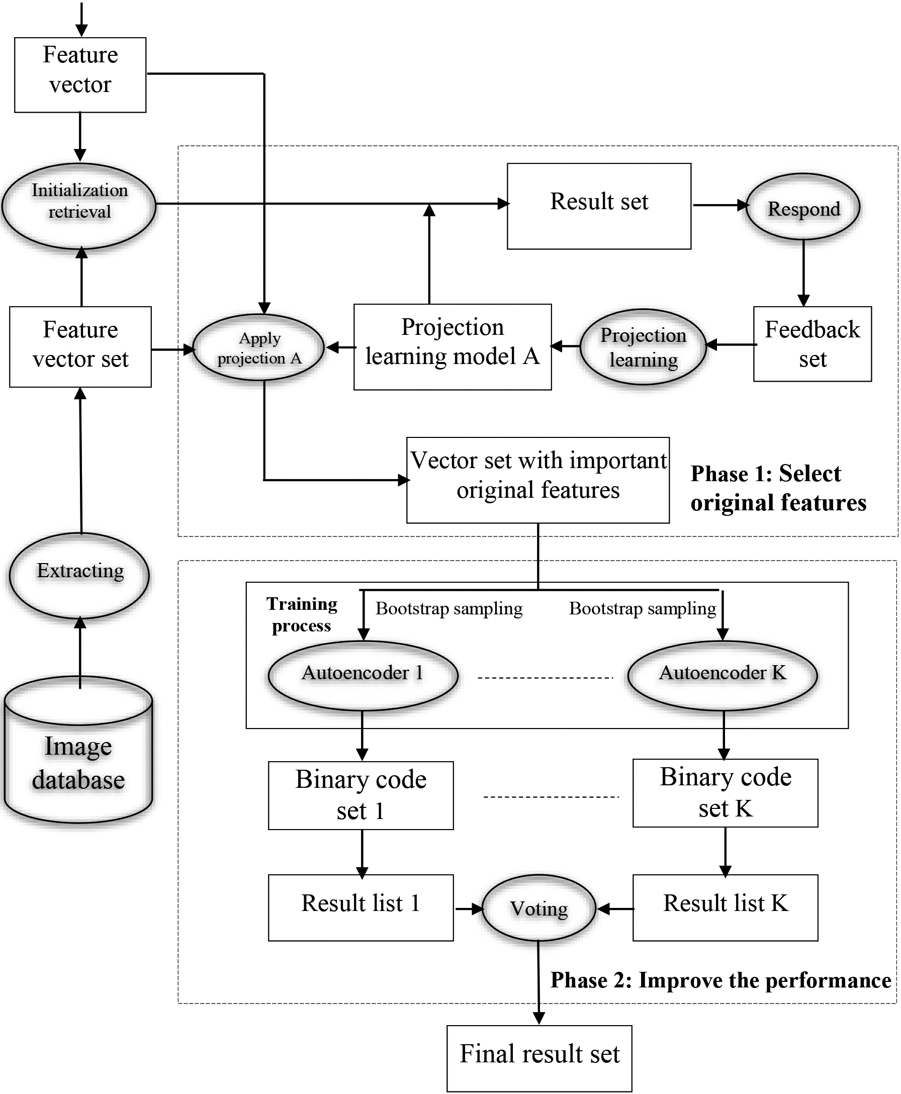

From the perspective of data flow, our proposed image retrieval method is described as shown in Fig. 1. The retrieval process begins by extracting the features of the query image. The features of the database images are pre-extracted according to some defined feature extraction procedure. Using these feature vectors together with a predefined image similarity measure (at the initial retrieval, the similarity measure is the Euclidean distance), the similarity between the query image and the database images is evaluated. Then, a set of images that are neighboring to the query image (At the initial retrieval, the set of neighboring images consists of images whose euclidean distance to the query image is below a given threshold) is selected and this set is sorted in descending order of similarity to obtain the result set. Our model is divided into two main phases corresponding to two dashed rectangles surrounded: Phase 1: Choose original features and Phase 2: Improve the performance.

With stage (1), the user responds on the retrieval result set to get the feedback set. This feedback set is also a training set, where the samples that are similar to the query image are considered positive, and the remaining samples (samples that are not similar to the query image) are negative. Based on this training set, the projection learning algorithm is performed to obtain the projection learning model A. This process continues until the user stops responding. Using projection learning model A on the feature vector set of the database image set, we obtain a set of vectors with important original features (this is also the output of Phase 1). It should also be noted here that, Phase 1 of our proposed model only returns the important features on the original feature space, but not the important features in the projection space (the meaning here is to avoid small-class size problem).

In the training process of Phase 2, we randomly select a subset of L feature vectors from the set of vectors that are the output of Phase 1 (note here that the samples in this subset are unlabeled). This subset will be used to train K deep autoencoders. During the training of deep autoencoders, we bootstrap the training set to train the corresponding K deep autoencoders.

After training K deep autoencoders, the candidates belonging to the database image set are passed through K deep autoencoders to obtain K sets of binary codes and then K result lists. An average voting mechanism is implemented to determine the similarity of each candidate. Next, we sort the candidates in descending order of similarity to get the final result set.

In the next section, we will focus on presenting the two main components of the model, which are “Select original features” and “Improve the performance”.

3.2 Select original features

The goal of this section is to reduce the data dimension but still solve the small-class size problem. In this section, we first introduce the $\ell_{2,1}$ norm constraint. Then, we present a projection learning model for selecting an important feature set that is suitable for the image retrieval problem for relevance feedback. It should also be noted here that this section includes the blocks: “Projection Learning”, “Projective Learning Model A”, “Sort features” and “Set of important feature vectors” in the model shown in Fig. 1.

A feature can be relevant, irrelevant, and redundant. The irrelevant and redundant features, which are taken into consideration during the classification process, can reduce the classification performance. The dimensionality of image data is often very high and often includes many redundant and irrelevant features [11]. Therefore, eliminating redundant and irrelevant features will simultaneously reduce the time and improve the precision for classification. This also improves the precision and reduces the retrieval time because the classification process is an important component of the image retrieval system.

We should note here that feature selection on the original feature space is an NP-Hard optimization problem on discrete spaces. To avoid facing the NP-Hard optimization problem, we reduce the optimization problem on the discrete space to the optimization problem on the continuous feature space, that is, we follow the transform-based dimensionality reduction approach [69].

Let ${A}=\left[{{a}_{1},{a}_{2},\ldots,{a}_{d}}\right]\in\mathbb{R}^{m\times d}$ represent the projection matrix. Project the sample ${x}$ from the original space to the projection space given by ${A}^{T}{x}$ . $\ell_{2,1}$ norm of ${A}$ [41] is given by

$\displaystyle||{A}||_{2,1}=\mathop{\sum}\limits_{i=1}^{m}\sqrt{\mathop{\sum}% \limits_{j=1}^{d}a_{ij}^{2}}=\mathop{\sum}\limits_{i=1}^{m}||{a}_{i}||_{2}$ (1)

A feature selection method can be obtained by minimizing the $\ell_{2,1}$ norm of the projection matrix as shown in [58]. In which, the $\ell_{2,1}$ norm constraint is used as a feature selection tool for classification. Whenever the rows of matrix A are zero or the $\ell_{2}$ norm is very small, the features corresponding to these rows are redundant and can be eliminated. To understand why the projection matrix ${A}$ can select important features, we analyze the structure of matrix ${A}$ . Let $a_{ij}$ be the components of the projection matrix $A$ . If feature ${x}_{j}$ is redundant, all elements of the $j^{\text{th}}$ row of ${A}$ must be zero, $\forall i,a_{ij}=0$ . This is done by minimizing $A_{2,1}$ . Therefore, forcing matrix A to have zero rows is to select features.

Feature extraction by imposing $\ell_{2,1}$ -norm constraint on the projection matrix of LDA is an effective approach [10, 56]. It can select and extract the most discriminating features and the extracted features can preserve the main energy of the original data. The learned projection matrix has good explanatory power for the features and has a good classification property for selecting the most important features. Learning a projection matrix is briefly described below.

First, we compute the matrix $S_{b}$ and $S_{w}$ :

$\displaystyle S_{b}=\frac{1}{n}\mathop{\sum}\limits_{i=1}^{c}n_{i}({{\mu}^{(i)% }-{\mu}})({{\mu}^{(i)}-{\mu}})^{T}$ (2) $\displaystyle S_{w}=\frac{1}{n}\mathop{\sum}\limits_{i=1}^{c}({\mathop{\sum}% \limits_{j=1}^{n_{i}}({{x}_{j}^{(i)}-{\mu}^{(i)}})({{x}_{j}^{(i)}-{\mu}^{(i)}}% )^{T}})$ (3)

Next, we solve the following optimization problem.

$\displaystyle\mathop{\min}\limits_{P,Q,E}Tr({A^{T}({S_{w}-uS_{b}})A})+\lambda_% {1}||A||_{2,1}+\lambda_{2}||E||_{1}$ (4) $\displaystyle s.t.\,X=PA^{T}X+E,P^{T}P=I$

Here ${A}\in\mathbb{R}^{m\times d}$ ( $d<m$ ) is the discriminant projection matrix. ${S}_{w}$ and ${S}_{b}$ are the within-class and between-class scatter matrices respectively. These two matrices ${S}_{w}$ and ${S}_{b}$ represent the use of labeled samples (user’s feedbacks). ${E}$ is the error matrix, which is represented as random noise (i.e. an image, after mapped to projection space, it will be split into two parts, clean image part and random noise part). $u$ is the constant that is used to equalize two scatter matrices. $\lambda_{1}$ and $\lambda_{2}$ are parameters, which are the trade-off in Eq. (4), used to determine the importance of related terms. $X=PA^{T}X+E$ and $P^{T}P=I$ make sure the original data can be restored well. $P\in\mathbb{R}^{m\times d}$ is an orthogonal reconstructed matrix. The alternating direction method of multipliers [3] is used to solve the optimization Eq. (4).

The feature extraction method according to the LDA approach has a limitation that is sensitive to the number of selected dimensions, that is, when the number of dimensions $d$ is very small, the discriminant information is not preserved. Meanwhile, the relevance feedback-based image retrieval problem is a binary classification problem ( $d<2$ ), that is, the number of dimensions obtained on the projection space is very small. This makes discriminant information not preserved. Therefore, the classification precision of the image retrieval methods according to the LDA approach, on the small-class size problem, is severely degraded. The projection matrix learned through the Eq. (4) above also follows the LDA approach, although it has been improved to lose as little discriminative information as possible. Therefore, in the image retrieval problem with relevance feedback, if we project the data to the projection space and perform the classification on this projection space, we will encounter the very small-class size problem as above.

To overcome the above very small-class size problem, we propose a projection learning model for selecting the important feature set on the original space, specifically as follows. We first learn a projection matrix ${A}$ by minimizing ${A}_{2,1}$ as in Eq. (4). Next, we use the projection matrix ${A}$ to remove the redundant features of the original space to get the important feature set. It should be noted here that the projection learning model results in a set of important features on the original space that helps to overcome the small-class size problem of the content-based image retrieval problem with relevance feedback. In this projection learning model ${A}$ and on the user’s feedback set, we compute $||{a}_{i}||_{2}$ , where ${a}_{i}$ is the $i^{\text{th}}$ row of matrix ${A}$ . In this model, the significance of the $i^{\text{th}}$ original feature is the value of $||{a}_{i}||_{2}$ . Then we sort the original features in descending order of $||{a}_{i}||_{2}$ respectively. The received feature vector set consists of the original features sorted in descending order of importance (redundant and irrelevant features are removed). The example below illustrates the selection of important feature sets.

Assume that we have the following data matrix ${X}$ and ${A}$ .

$\displaystyle{X}=\left[{{\begin{array}[]{*{20}c}x_{11}&x_{12}&x_{13}&x_{14}\\ x_{21}&x_{22}&x_{23}&x_{24}\\ x_{31}&x_{32}&x_{33}&x_{34}\\ \end{array}}}\right]\text{ and }{A}=\left[{{\begin{array}[]{*{20}c}a_{11}&a_{1% 2}\\ a_{21}&a_{22}\\ a_{31}&a_{32}\\ \end{array}}}\right]$

Suppose that after calculation, we have $||{a}_{3}||_{2}>||{a}_{2}||_{2}>||{a}_{1}||_{2}$ and we want to get $k=$ 2 most important features, then we get

$\displaystyle{A}_{k}=\left[{{\begin{array}[]{*{20}c}a_{31}&a_{32}\\ a_{21}&a_{22}\\ \end{array}}}\right]\text{ and }{X}_{k}=\left[{{\begin{array}[]{*{20}c}x_{31}&% x_{32}&x_{33}&x_{34}\\ x_{21}&x_{22}&x_{23}&x_{24}\\ \end{array}}}\right]$

The projection learning algorithm for selecting the set of vectors with important features is summarized in Algorithm 1.

Algorithm 1: Selecting the set of vectors with important features.
Input: – Training sample matrix X, label matrix Y
– Parameters $\lambda_{1}$ , $\lambda_{2}$ , number of important features $k$
Output: – Projection Matrix A
– Set of vectors with important features ${X}_{k}$
Step 1: Calculate $S_{b}$ according to Eq. (2); Calculate $S_{w}$ according to the Eq. (3)
Step 2: Solve the optimization Eq. (4) according to [3] to get the projection matrix ${A}$
Step 3: Calculate $\|\|{a}_{i}\|\|_{2},i=1,2,\ldots,m$ of the projection matrix ${A}$
Step 4: Sort $m$ rows of ${X}$ in descending order of $\|\|{a}_{i}\|\|_{2}$ . Construct ${X}_{k}$ consisting of $k$ rows on the top of ${X}$ .
Step 5: Return A and ${X}_{k}$

Computational complexity

In Algorithm 1, Step 2 has the highest computational cost. In this step, the computational cost is to solve the Eq. (4). The computational cost (Wen et al., 2018) to find the solution of Eq. (4) is ${{\rm O}}({\textit{Inter}({m^{2}n+m^{3}+2m^{2}d+d^{3}})})$ , where $m$ is the number of dimensions of the original space, $n$ is the number of training samples, $d$ is the number of dimensions of the projection space, and Inter is the number of iterations. Since the algorithm, which finds the solution of E.q (4), usually converges in about 10 iterations, we can consider Inter as a constant and can be ignored. In the image retrieval problem with relevance feedback, the number of feedback samples $n$ and the number of dimensions $d$ of the projection space are usually very small, so we can consider them constant. Thus, the computational complexity of Algorithm 1 is ${{\rm O}}({m^{3}})$ .

3.3 Improve the performance

In Section 2.2, we have obtained a set of vectors with important features. Although redundant and irrelevant features have been removed, the cost of image retrieval is still very high, which is not suitable for searching in a large-scale dataset. The reason for this is that because the remaining features have real values, it must use a traditional linear search (or exhaustive search) strategy. The following sections demonstrate how to achieve the goal of improving image retrieval speed and precision on large-scale datasets.

Speed up image retrieval process

Autoencoder can adaptively learn the structure of data and efficiently represent the data. The output of the autoencoders is converted to low-dimensional binary codes, which are well suited for large-scale datasets and data diversity. In addition, autoencoder overcomes poor generalization and expensive design costs.

We convert feature vectors to low-dimensional binary codes. The autoencoder consists of an adaptive multilayer encoding network, which maps high-dimensional data to low-dimensional code, and a similar decoder network, which recovers data from the code. The autoencoder network architecture includes hidden layers for encoders, decoders, and a bottleneck layer. We assume the final output of the bottleneck layer $H$ consists of $h$ hidden neurons each with an output value of 0 or 1. In this case, images that are similar will produce similar binary activations. We replace the bottleneck layer with a hidden layer $H$ as shown in Fig. 2. Note here that the threshold value used is 0.5, ie if $\textit{Output}({H_{j}})>0.5$ then thì $H_{j}=1$ , otherwise $H_{j}=0$ with $j=1,2,\ldots h$ .

The entire autoencoder network is trained with gradient descent through minimizing the error between the original data and its reconstructed data. Note here that all unlabeled samples (image database feature vectors) are utilized. That is also why our proposed method is called semi-supervised. As in [26], the entire training process of an autoencoder includes pretraining and fine-tuning. As shown in Fig. 2, during pretraining, we create the encoder network by learning a stack of restricted boltzmann machines (RBM) with standard contrastive divergence specified in [20]. Each RBM has only one hidden layer and it is trained using the hidden activations of the previous RBM as input. By stacking RBMs, we can obtain better initialization weights for gradient descent. We then unroll the encoder network to generate an autoEncoder, which is initialized with the weights from the stacked RBMs and fine-tuned by reconstruction errors via backpropagation. We train the autoencoders on a subset of size L (in our experimental case we choose L $=$ 1000), which is randomly selected from the large-scale dataset. Note here that all unlabeled samples of the image subset are mined. Our proposed method is called semi-supervised because its Phase 1 uses labeled samples to select important features while Phase 2 uses unlabeled samples.

Figure 2.

Proposed deep autoencoder model.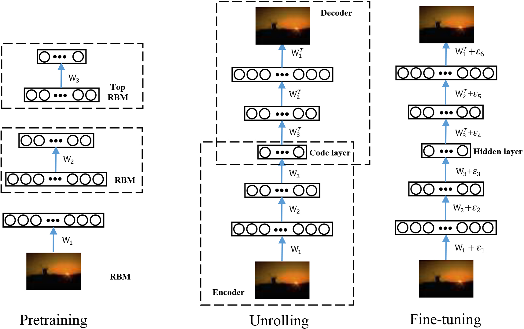

Improve precision of image retrieval

As tested in [68], neural networks are unstable models, and shuffling the training set can cause significant changes in the built model, especially when the distribution of samples is uneven. Bagging is an effective associative learning strategy for improving unstable predictive models. In our method, many new training sets are generated through bootstrap cloning of the original training set and each of them is used to train a corresponding autoEncoder. By reselecting the training set, bagging increases the differences in the integration of different autoencoders. This enhances the generalizability of autoencoders. So we can get multiple descriptions for each object with these autoencoders. We can compute multiple similarity for each pair of objects and obtain a lookup result set by ranking the average measure values. Training many autoencoders will take a long time, but our method uses bagging, which can compute in parallel, so efficiency is still guaranteed.

The K deep autoencoders training algorithm is summarized in Algorithm 2.

Algorithm 2: Training K deep autoencoders.
Input: – ${q}_{k}$ : Vector with important original features of the query image
– ${X}_{k}$ : Vector set with important original features of the database image set
Output: – Training model for K deep autoencoders.
Step 1: Randomly select a subset of ${L}_{k}$ feature vectors of ${F}_{k}$
Step 2: Bootstrap K training set ${L}_{k}$
Step 3: Pre-training by a model consisting of a stack of RBMs for K bootstrap replica sets
Step 4: Unrolled RBMs to create K deep autoencoders.

3.4 Proposed image retrieval algorithm

This section presents the overall algorithm for image retrieval. This overall algorithm calls Algorithm 1 to generate a set of vectors with important features, i.e. each feature vector includes important features on the original feature space of the image database. On this set, the overall algorithm randomly selects a subset including L candidates to train K deep autoencoders by calling Algorithm 2.

To improve precision, in addition to using bagging autoencoder strategy in algorithm 2, here we will use coarse-to-fine retrieval strategy. In this strategy, we first find a set of candidate images based on a quick comparison of binary compact codes over the Hamming distance. Then, on the list of candidate images, we filter out the images based on comparing the real value vectors (output of Phase 1) by Euclidean distance.

The proposed image retrieval algorithm is summarized in Algorithm 3.

Algorithm 3: BCFIR
Input: ${\rm{\bf F}}$ : feature set of database images, q: query image vector, N: Number of images returned at each iteration
Output: $S$ : Result set
Step 1: Query by sample image q by euclidean distance and get N top images to get initial retrieval result set $I$
Step 2: Repeat
Step 2.1: User responds on set $I$ to obtain the feedback set ${RF}$ .
Step 2.2: Run Algorithm 1 to get a projection learning model ${A}$ and a set of vectors with important features ${X}_{k}$ .
until (User stops responding);
Step 3: Apply projection A on the set of feature vectors of the image database to obtain a set of vectors with important original features.
Step 4: Call Algorithm 2 to train K deep autoencoders.
Step 5: Apply the vector set with the important original features of the database image set to K deep autoencoders to obtain K binary code sets and then K result lists.
Step 6: Determine the similarity of the candidates in the resulting list according to the Hamming distance and the average voting mechanism.
Step 7: Sort the candidates in descending order of similarity and take the $N^{\prime}$ ( ${N}^{\prime}>N$ ) candidates at the top of the list as the resulting image set $S^{\prime}$ .
Step 8: Apply coarse-to-fine strategy: On the result set $S^{\prime}$ , we calculate the similarity of $N^{\prime}$ candidates with $q$ vector with important original features by Euclidean distance.
Step 9: Sort the candidates in descending order of similarity and take the top $N$ candidates from the list S’ as the resulting image set $S$ .
Step 10: Return S;

4. Experimental results

In this section, we present experiments to evaluate the performance of our proposed image retrieval method. The first experiment reports the comparisons of our proposed method with typical image retrieval methods. This is to show that the proposed method has higher overall precision than the other methods. The second experiment tests the average execution time of the proposed method. The third experiment is to consider the efficiency when removing redundant and irrelevant features. The last experiment is to demonstrate the effectiveness of the method in solving the very small-class size problem in image retrieval with relevant feedback. The final experiment on the large-scale datasets is to demonstrate the precision and speed of the proposed method.

In the original feature space, the Euclidean Distance, which is between the query image and the database image, is used in calculating the precision of the Baseline method and the initial retrieval stage.

4.1 Image database

Corel Image Database

The Corel photo gallery is an image database that has been widely used to evaluate the performance of CBIR systems [48, 71]. Therefore, we use this dataset to perform an empirical evaluation of our proposed method. Based on the ground truth, the images that are not suitable for image retrieval in the Corel photo gallery are removed, we get a Corel image database of 10,800 images with 80 semantic concepts. In this image database, each semantic concept consists of 100 or more images, and the size of each image is 120 $\times$ 80 or 80 $\times$ 120. Figure 3 shows some sample images in the Corel image database. This image database will help us automatically evaluate the retrieval performance.

Figure 3.

Some representative images of 5 semantic concepts in Corel.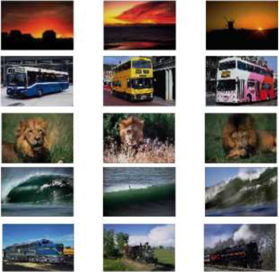

Images in an image database are represented by a set of low-level features in 190-dimensional space. Thus, each image is represented by a feature vector consisting of 190 components. Of these 190 components, there are 102 components for color features and 88 components for texture features. With 102 components for color features, it includes 6 components for the color moment, 32 components for color histogram, and 64 components for color correlation. In addition, the 88 components for the texture feature are composed of 48 Gabor components and 40 Wavelet components.

SIMPLIcity Image Database

The SIMPLIcity database consists of 1000 images, which are divided into 10 semantic concepts. The size of each image in this set is 256 $\times$ 384 or 384 $\times$ 256. Figure 4 includes several images that represent the five semantic concepts in this image database. The images in the image database are represented by a set of low-level features in 278-dimensional space, which consists of 128 components for color features and 150 components for edge features.

Figure 4.

Some representative images of five semantic concepts in SIMPLIcity.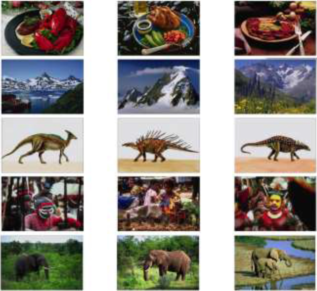

The CIFAR-10 dataset

The CIFAR-10 database consists of 60000 images, which are divided into 10 semantic concepts with 6000 images for each semantic concept. The size of each image in this set is 32x32. Figure 5 includes some of the images in this image database.

Figure 5.

Some representative images of 5 semantic concepts in CIFAR-10.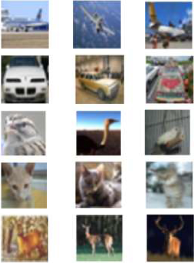

4.2 Performance evaluation

In this section, we use the precision and precision-scope curves [21] to evaluate the effectiveness of the image retrieval methods. Where, the scope is the top $N$ images returned to the user, and precision is defined as the ratio of the number of relevant images over the $N$ returned images. In the experiment, because the output of Phase 1 of the proposed model in Fig. 1 includes only vectors with important features, while we want to demonstrate the efficiency of solving small-class size problem only for Phase 1, so we have to rely on a powerful and popular classifier that is SVM. We also evaluate the methods using fourfold cross validation, i.e. we divide the image database into four equally sized subsets. Whenever cross validation is performed, the query set is also a selected subset while the remaining three subsets are used as the database for image retrieval. Precision is understood as the average precision of fourfold cross-validation. In the empirical evaluation in this section, the top 100 images that are returned to the user are important because each semantic concept in the Corel and SIMPLIcity image sets contains about 100 images.

4.2.1 Experiment on the overall performance of the proposed method

In this section, to show the precision of the proposed method, we divide the methods used for comparison with our method into two groups: the first comparison group are methods that do not use deep learning; The second group of comparisons are methods that use hashing or that use deep learning. The reason for this grouping is to compare with our proposed method which covers only phase 1 with SVM (called BCFIRPhase1) and our proposed method which includes enough two phases (ie, BCFIR).

The first comparison group includes Baseline, BDA, DSSA, DLRPIR methods. Baseline is an image retrieval method that only uses Euclidean distance to measure the similarity between the query image and the database image. It retrieves the images that are neighboring to the query image based on the Euclidean distance and does not use any learning mechanism in the retrieval process. This method is used to show the effectiveness of relevance feedback in image retrieval. We compare the proposed method with methods BDA [75] and DSSA [73] because they are very popular traditional relevance feedback image retrieval methods. DSSA uses relevant feedback to learn a discriminant projection matrix, which projects data from the original space to the projection space. BDA is an image retrieval scheme with relevance feedback based on discriminant analysis, it reduces the influence of sample imbalance. We also choose DLRPIR for the comparison because it can mitigate the small-class size problem. DLRPIR is an image retrieval method, which uses the same similarity measure and feedback mechanism as our proposed method. What is different from our method is that DLRPIR uses a Discriminative Low-Rank Projection method, called DLRP [29], to project the original data into a projection space. It then performs classification on this projection space to classify the images. The reason we use the DLRPIR method for comparison is because it can mitigate the small-class size problem.

The methods belonging to the second group of comparisons are NSCM (new similarity calculation method) [50], and LSH [2]. We chose the NSCM method for our comparison because it is a method that has state of the art performance. We chose LSH because it is one of the most popular data-independent hashing methods. LSH embeds similar images into similar binary codes with high probabilities.

In the experiment, we set the values of the parameters for the methods of the first group as follows. With DSSA, the number of dimensions of the projection space is 8 because this is its optimal dimension [22]. In DLRP, we set the value of both parameters $\lambda$ and $\alpha$ , which are chosen to be $10^{-4}$ because this value is in the optimal range [29], and we also choose the number of dimensions of the subspace to be 135 because 135 is within the optimal value of DLRP and the same optimal number of dimensions with our proposed method. In our proposed method, the values of the parameters $\lambda_{1}$ and $\lambda_{2}$ were chosen as 0.001 because this is the recommended optimal value [56]. Besides, in the proposed method, the number of dimensions is chosen as 135 because this value is approximately the optimal dimension (70% of the total number of original features) of the original feature set as shown in [10]. With NSCM, the length of binary compact codes is 32 or 48 bits. For comparison purposes, 32 bits or 48 bits are also lengths that the BCFIR method chooses for performance evaluation.

4.2.1.1 Results on Corel

Precision test of the proposed method with the first comparison group

After initial retrieval, we get an initial retrieval result set of 100 images. On this set of 100 images, the user response to obtain a feedback set, which consists of positive and negative samples. Next, we apply BDA, DSSA, DLRPIR and BCFIRPhase1 methods to rerank the images in the image database. After ranking the images, we get four sets of search results of the four methods respectively. Figure 6 shows the average precision, at the top 100 images for the first iteration, of the five methods. Here, we give precision for the first loop because in image retrieval with relevance feedback, the first loop is the most important. It is also important to note here that average precision is the average precision of all queries, each of which corresponds to an image in the image database. Taking each of the entire database image set as a query image and then calculating the average precision of all queries will more accurately reflect the performance of the method because it includes very bad queries (returns only a few relevant images).

The results in Fig. 6 show us that the Baseline method gives the lowest precision. The reason for this is that the Baseline method does not have a learning mechanism to reduce the semantic gap between the high-level semantic concept and the low-level visual feature, it only calculates the Euclidean distance between the query image and the database image on 190-dimensional feature space. Regardless of the Baseline method, the precision of the BDA method is the lowest of the four methods. The reason for this is that the projection space of BDA is low discriminant and is greatly affected by the small-class size problem. The precision of the DSSA method is superior to that of BDA because it can find a projection space that is more discriminative than that of BDA. The DLRPIR method gives a higher precision than that of BDA and DSSA because its projection space is less prone to loss of discriminability when the dimensionality is very low, i.e. it reduces the effect of the small-class size problem. The precision of our proposed method is the highest among the four methods because it effectively solves the problem of small-class size, and solves the problem of small sample size.

Table 1 shows the average precision, at the top 100 images for the first iteration, of each of the 20 semantic concepts. It should also be noted here that the precision of a semantic concept here is the average precision of all queries, where each query corresponds to an image in that semantic concept. From Table 1, we see that, in only 3 out of 20 semantic concepts, the precision of our proposed method is lower than the other three methods, while there are up to 17 semantic concepts (the highlights in Table 1), the precision of our method is higher than other methods.

Table 1
Average precision of 20 semantic concepts of the five methods

No.	Concept	Baseline	BDA	DSSA	DLRPIR	BCFIRPhase1
1	‘art_antiques’	12.19	22.72	24.91	24.23	27.72
2	‘art_dino’	66.89	74.09	86.62	81.79	91.08
3	‘fitness’	51.52	71.67	85.81	82.15	90.09
4	‘obj_bus’	19.34	40.21	42.42	59.75	61.47
5	‘obj_decoys’	47.33	61.63	72.79	67.67	75.49
6	‘obj_moleculr’	15.81	31.22	34.41	35.67	37.18
7	‘obj_train’	22.02	42.12	44.72	45.43	48.47
8	‘pl_foliage’	3.86	6.89	27.83	22.45	23.88
9	‘sc_firewrk’	29.33	59.57	74.65	72.76	75.21
10	‘sc_indoor’	15.45	28.33	33.45	34.68	37.42
11	‘sc_sunset’	18.30	51.36	59.64	72.78	78.91
12	‘texture_2’	33.52	46.33	53.52	53.78	55.91
13	‘texture_6’	50.33	61.80	76.89	86.91	93.86
14	‘wl_buttrfly’	11.19	24.93	29.97	35.73	36.39
15	‘wl_deer’	6.52	13.15	24.54	35.14	27.09
16	‘wl_eagle’	8.37	18.03	25.21	26.31	28.67
17	‘wl_horse’	13.83	25.26	28.45	29.59	31.29
18	‘wl_owls’	27.67	36.17	38.38	45.29	48.04
19	‘wl_roho’	6.68	14.76	21.89	18.16	19.83
20	‘woman’	30.74	59.46	63.74	71.54	72.27

Figure 6.

Average precision of the 5 methods in the top 100.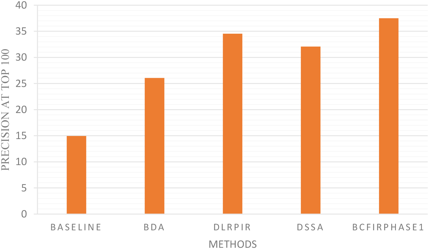

Figure 7 shows the precision-scope curves for the first response iteration. The methods are tested on scopes 20, 40, 60, 80, and 100. According to the scopes, the precision of our method is higher than that of the other four methods. As shown in Fig. 7, the precision of DLRPIR is higher than that of DSSA but its that is lower than our method.

Query processing time test with the first comparison group

This experiment aims to test the query execution time of the proposed method compared to the remaining methods. As shown in Table 2, the average query time for all four methods is fast, which is less than 0.05 s for the first feedback iteration. The average query time of our method is slower than that of the DSSA method and is comparable to that of DLRPIR. The average query time of DSSA is faster than that of our method because DSSA can be obtained the mapping matrix by using the Eigenvalue decomposition. Our method and DLRPIR use the same algorithm to find the projection matrix, so the average query time of our method is equivalent to that of DLRPIR. Average query time in Table 2 made on the computer, configured as 3.1 GHz Dual-Core Intel Core i5 Catalina machine with 8 GB 2133 MHz LPDDR3 memory.

Table 2

Average time for executing a query

Method	Average execution time (s)
	Feedback iteration 1	Feedback iteration 2
BCFIRPhase1	0.067	0.078
DLRPIR	0.068	0.077
DSSA	0.062	0.071
BDA	0.064	0.079

Figure 7.

Average precision-scope curves of the different methods.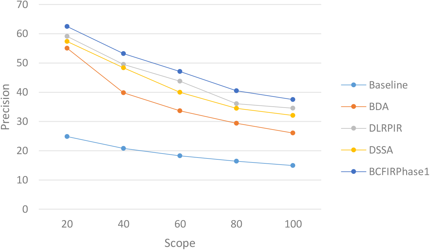

4.2.1.2 Results on the set of SIMPLIcity

This section shows the precision of the proposed method compared with the methods of the first comparison group on the set of SIMPLIcity.

The average precision-scope curves of the BDA, DLRPIR, DSSA, and proposed methods are shown in Fig. 8. Methods are tested on scopes 20, 40, 60, 80, and 100 for the first iteration. According to the results in this figure, the average precision-scope curve of the proposed method is better than the rest.

Thus, on two benchmark data sets, the performance of our method is higher than that of BDA, DLRPIR, and DSSA. This information helps us to confirm that the proposed method is very effective.

Figure 8.

Average precision-scope curves of the different methods.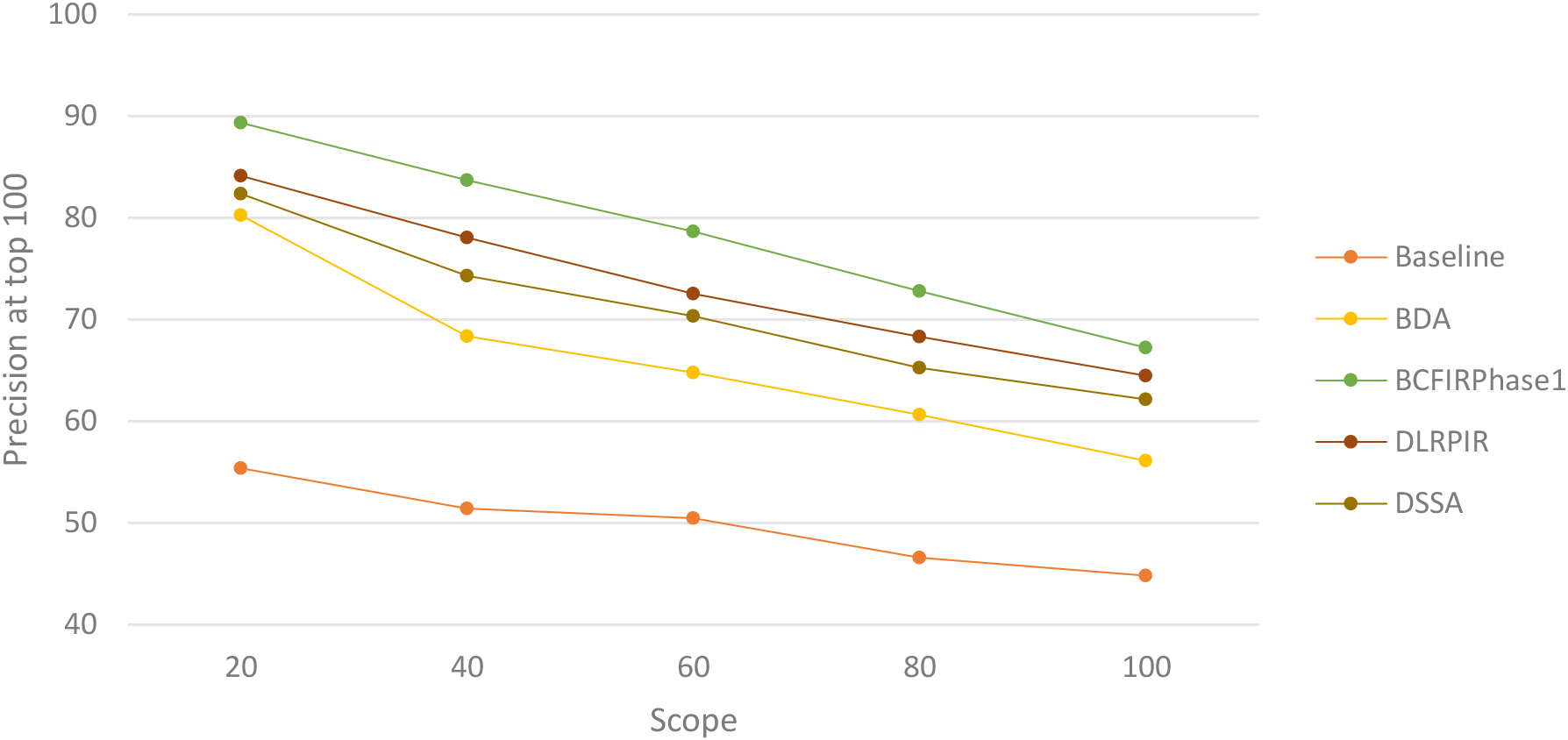

4.2.2 Experiment on efficiency when removing redundant features and solving small-class size problem

Effectiveness when removing redundant and irrelevant features.

Because the effectiveness of our proposed method relies on removing redundant and irrelevant features, so we show this experimentally in this section. To show that eliminating redundant and irrelevant features is effective for image retrieval with relevance feedback using classification learning, we conduct the test under the following scenario. We build an image retrieval method with relevant feedback using SVM, called SVMRF. The SVMRF method uses the received feedback set to train an SVM model and then uses this SVM model to rank the images to obtain the result set. When applying SVMRF on the original feature space, which consists of 190 dimensions, it is called SVMRF_190. Also SVMRF but applies it an important feature set (the result of Algorithm 1), which consists of 135 dimensions, it is called SVMRF_135. The precision of SVMRF_190 and SVMRF_135 is shown in Fig. 9. It should also be noted here that precision is calculated on the top 100 returned images and for the first iteration. As shown in the figure, although SVMRF_135 has eliminated 55 dimensions, the precision of SVMRF_135 is still higher than that of SVMRF_190. Thus, we can see that the 55 dimensions of the feature space are redundant and irrelevant.

Figure 9.

Precision of SVMRF_190 and SVMRF_135.

Figure 10.

Results for query image.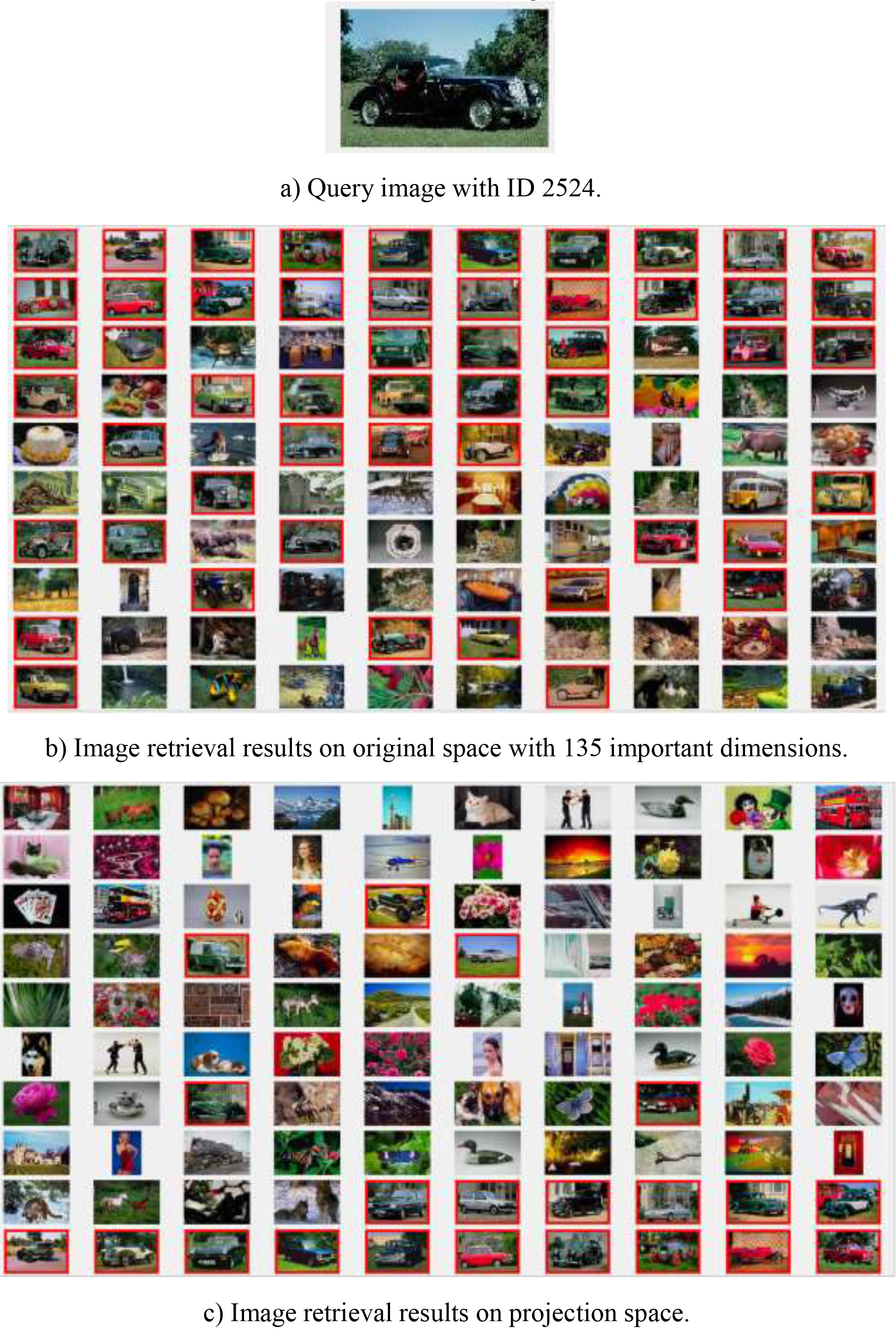

Effectiveness when dealing with small-class size problems.

An important contribution of our proposed method is that it is not affected by the small-class size problem. To illustrate this problem visually, we randomly select an image in the Corel database as the query image, it has ID 2524 and belongs to the concept of “obj_car”. We perform this image retrieval process on the original space with 135 important dimensions and also perform this on the projection space. Figure 10 shows the result with ID 1386, Fig. 10a is the query image ID 2524, Fig. 10b shows the result on the original space, and Fig. 10c shows the result on the projection space. As shown in Fig. 10b, out of 100 returned images, we get 52 relevant images, which rank very high. Figure 10c shows us that, out of the 100 returned images, we get only 21 relevant images, which have low rankings.

Next, we conduct experiments to show the advantages of the proposed method. In the test scenario, our proposed method SDAIR is performed on both the projection space and on the important feature set for comparison purposes. BCFIRPhase1 is applied on projection space for dimensions that include 19, 57, 95, and 135. On projection space, the methods BCFIRPhase1_P19, BCFIRPhase1_P57, BCFIRPhase1_P95, and BCFIRPhase1_P135, which have dimensions of 19, 57, 95, and 135, respectively. It should also be noted here that BCFIRPhase1 is a retrieval method on the original space with the removal of 55 redundant dimensions as shown in Fig. 6. The precision of the methods is shown as shown in Fig. 11. Figure 11 shows us that, although the number of dimensions of BCFIRPhase1_P135 and BCFIRPhase1_135 are the same, the precision of BCFIRPhase1_P135 is lower than that of BCFIRPhase1_135 by approximately 10%. The reason that the precision of BCFIRPhase1_135 is so much higher than that of BCFIRPhase1_P135 is because the BCFIRPhase1_135 method is not affected by the small-class size problem. As this figure shows, the precision of BCFIRPhase1_P19, BCFIRPhase1_P57, BCFIRPhase1_P95 are equivalent to each other and also equivalent to BCFIRPhase1_P135. The reason for this is because performing the retrieval on the projection space is severely affected by the small-class size. Thus, we can confirm that our proposed method is not affected by small-class size.

Figure 11.

Precision of BCFIRPhase1_135 on original space and BCFIRPhase1 on projection space.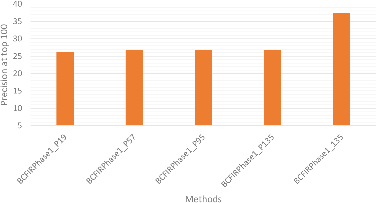

4.2.2.1 Results on the CIFAR-10

Our goal in this section is to compare the BCFIR’s performance with the state of the art method, which uses deep learning (of the second comparison group) on large image set. When comparing on 32-bit and 48-bit lengths, our proposed method is named BCFIR32b and BCFIR48b. When BCFIR32b and BCFIR48b are applied to four autoencoders ( $L=4$ ), they are named BCFIR32b_4a and BCFIR48b_4a, respectively.

In this experimental part, we randomly select 1000 images in the image set as query images. We also take the top 100 images as the returned list of images. Note here that, in our method, we choose the number of images in the candidate list as 300. Thus, the top 100 resulting images are selected from 300 candidate images.

Table 3

Precision of different methods

No.	Method	Precision
1	LSH	60.23%
2	NSCM32b	69.6%
3	BCFIR32b_4a	68.75%
4	NSCM48b	70.07%
5	BCFIR48b_4a	70.11%
6	NSCM128b	70.65%
7	BCFIR128b_4a	70.72%

From Table 3 we can see, our method BCFIR32b_4a and BCFIR48b_4a have higher precision than that of LSH which is about 8% and 10% respectively. This shows the precision of the proposed method. On a code length of 32 bits, our proposed method BCFIR32b_4a has slightly less precision than that of NSCM32b. The reason for this may be because the length of the code is too low while phase 1 of the proposed method has removed some dimensions of the feature vector on the original space. With a code length of 48 bits, our proposed method has slightly higher precision than that of NSCM48b. However, when the length of the code is 128, the precision of our method is higher than that of NSCM. The reason for the effectiveness of our method compared to the NSCM method is because our method solves the following problems: (1) small-class size problem; (2) it can efficiently learn binary codes; (3) use bootstrap cloning strategy with effective bagging; (4) take advantage of unlabeled samples in the retrieval process; and (5) use an efficient coarse-to-fine retrieval strategy. With the first response, the average time to perform 01 query image on original space with 95 dimensions for BCFIRPhase1_95 is 12 s while our proposed method BCFIR128b_4a is only 2.58 s.

5. Conclusion

In the problem of image retrieval with relevance feedback, we have to reduce the data dimensionality and still have to solve the small-class size problem which is a difficult task. In this paper, we solve this problem by selecting important original features and performing classification based on them. In order not to have to solve the NP-Hard problem in feature selection, instead of solving the combinatorial optimization problem, we reduce it to an optimization problem on the continuous feature space (according to the transform-based dimensionality reduction approach).

In addition, although recent works on image retrieval with relevance feedback have shown many improvements in performance, they yield low performance for large-scale datasets. Our proposed method BCFIR gives good performance on large-scale datasets. In addition to mapping real-valued features to short binary codes and using Hamming distance measure to speed up image retrieval, our proposed method also learns a good parameter transfer model, and apply a bagging learning strategy to improve the generalizability of deep autoencoders.

In addition, in the image retrieval problem with relevance feedback, the number of user feedback samples is usually small. This limits the performance of pure supervised learning methods. Our proposed method BCFIR takes advantage of both labeled and unlabeled samples. In particular, labeled samples need only be used for the selection of important original features in Phase 1, while Phase 2 uses unlabeled samples to train deep autoencoders.

Experimental results on CIFAE-10, Corel, and SIMPLIcity show that the proposed method generates state of the art image retrieval performance on standard benchmarks. These experimental results are in agreement with our proposal and analysis.

Footnotes

Acknowledgments

This research is funded by “Research on content-based image retrieval using relevance feedback with sparse representation classification” of Institute of Information Technology (IOIT), Vietnam Academy of Science and Technology (VAST) under grant number code CS21.04. This research was also supported by the research support program Offer for senior researchers in 2022 under grant no. NVCC02.01/22-22.

References

Guillaume

and Yoshua

, What regularized auto-encoders learn from the data-generating distribution, Journal of Machine Learning Research 15(1) (2014), 3563–3593.

Andoni

and Indyk

, Near-optimal hashing algorithms for approximate nearest neighbor in high dimensions, in FSCS, 2006.

Boyd

Parikh

Chu

Peleato

and Eckstein

, Distributed optimization and statistical learning via the alternating direction method of multipliers, Foundations and Trends in Machine Learning 3(1) (2011), 1–122.

Chen

Weinberger

K.Q.

Sha

and Bengio

, Marginalized denoising auto-encoders for nonlinear representations, in: Proceedings of International Conference on Machine Learning, 2014, pp. 1476–1484.

Clemmensen

Hastie

Witten

and Ersboll

, Sparse discriminant analysis, Technometrics 53(4) (2011), 406–413.

Datta

Joshi

and Wang

J.Z.

, Image retrieval: Ideas, influences, and trends of the new age, ACM Computing Surveys 40(2) (2008), 1–60.

Deng

Chen

Liu

Gao

and Tao

, Triplet-based deep hashing network for cross-modal retrieval, IEEE Trans. Image Process. 27(8) (2018), 3893–3903.

Donoho

, High-dimensional data analysis: the curses and blessings of dimensionality, in: AMS Conference on Math Challenges of the 21st Century, 2000, pp. 1–33.

Dorfer

Kelz

and Widmer

, Deep linear discriminant analysis, in: International Conference on Learning Representations, 2015, pp. 1–13.

10.

Fadi

and Khoder

, Linear embedding by joint Robust Discriminant Analysis and Inter-class Sparsity, Neural Networks 127 (2020), 141-159.

11.

Duda

R.O.

Hart

P.E.

and Stork

D.G.

, Pattern Classification, second ed. Wiley-Interscience, 2000.

12.

Duda

R.O.

Hart

P.E.

and Stork

D.G.

, Pattern classification, Wiley, New York, 1973.

13.

Fan

and Zhang

, Local linear discriminant analysis framework using sample neighbors, IEEE Transactions on Neural Networks 22(7) (Jul. 2011), 1119–1132.

14.

Fang

Lai

and Wong

W.K.

, Learning a nonnegative sparse graph for linear regression, IEEE Transactions on Image Processing 24(9) (2015), 2760–2771.

15.

Feng

Wang

and Ahmad

, Correspondence autoencoders for cross-modal retrieval, ACM Transactions on Multimedia Computing, Communications, and Applications 12, 1s, Article 26 (2015), 22 pages.

16.

Hameed

I.M.

Abdulhussain

S.H.

and Mahmmod

B.M.

, Content-based image retrieval: A review of recent trends, Cogent Engineering, 2021, 1927469.

17.

Han

Zhang

Wen

Guo

Liu

and Li

, Two-stage learning to predict human eye fixations via SDAEs, IEEE Transactions on Cybernetics 46(2) (2016), 487–498.

18.

and Niyogi

, Locality preserving projections, in: Advances in Neural Information Processing Systems, 2004, pp. 153–160.

19.

Cai

Yan

and Zhang

H.-J.

, Neighborhood preserving embedding, in: IEEE International Conference on Computer Vision. IEEE, 2005, pp. 1208–1213.

20.

Hinton

, A practical guide to training restricted boltzmann machines, Momentum 9(1) (2010), 926.

21.

Huijsmans

D.P.

and Sebe

, How to complete performance graphs in content-based image retrieval: Add generality and normalize scope, IEEE Trans. Pattern Analysis and Machine Intelligence 27(2) (2005), 245–251.

22.

Huu

Q.N.

Viet

D.C.

and Thuy

Q.D.T.

, Semantic class discriminant projection for image retrieval with relevance feedback, Multimedia Tools and Applications 80(10) (2021), 15351–15376.

23.

Indyk

and Motwani

, Approximate nearest neighbors: Towards removing the curse of dimensionality, in Proc. STOC, 1998, pp. 604–613.

24.

Jolliffe

I.T.

, Principal Component Analysis, 2nd ed. New-York: Springer-Verlag, 2002.

25.

Kirby

and Sirovich

, Application of the karhunen-loeve procedure for the characterization of human faces, IEEE Transactions on Pattern analysis and Machine intelligence 12(1) (1990), 103–108.

26.

Krizhevsky

and Hinton

G.E.

, Using very deep autoencoders for content-based image retrieval, in ESANN. Citeseer, 2011.

27.

Kulis

and Grauman

, Kernelized locality-sensitive hashing, IEEE Trans. Pattern Anal. Mach. Intell. 34(6) (2012), 1092–1104.

28.

Lai

Jin

and Zhang

, Human gait recognition via sparse discriminant projection learning, IEEE Transactions on Circuits and Systems for Video Technology 24(10) (2014), 1651–1662.

29.

Lai

Bao

Kong

Wan

and Yang

, Discriminative low-rank projection for robust subspace learning, International Journal of Machine Learning and Cybernetics, 2020, 1–14.

30.

Allinson

Tao

and Li

, Multitraining support vector machine for image retrieval, IEEE Transactions on Image Processing 15(11) (2006), 3597–3601.

31.

Wang

and Zhang

, Linear discriminant analysis using rotational invariant l1 norm, Neurocomputing 73(13–15) (2010), 2571–2579.

32.

Liu

Tang

and Lu

, Robust structured subspace learning for data representation, IEEE Transactions on Pattern Analysis and Machine Intelligence 37(10) (2015), 2085–2098.

33.

W.-J.

Wang

and Kang

W.-C.

, Feature learning based deep supervised hashing with pairwise labels, in Proc. IJCAI, 2016, pp. 1711–1717.

34.

Lin

Chen

C.-S.

and Zhou

, Learning compact binary descriptors with unsupervised deep neural networks, in Proc. CVPR, 2016, pp. 1183–1192.

35.

Liong

V.E.

Wang

Moulin

and Zhou

, Deep hashing for compact binary codes learning, in Proc. CVPR, 2015, pp. 2475–2483.

36.

Liu

Wang

Kumar

and Chang

S.-F.

, Compact hyperplane hashing with bilinear functions, in Proc. ICML, 2012, pp. 467–474.

37.

Liu

and Shao

, Multiview alignment hashing for efficient image search, IEEE Transactions on Image Processing 24(3) (2015), 956–966.

38.

Liu

Wang

Zha

Z.J.

and Hong

, Cross-modality feature learning via convolutional autoencoder, ACM Transactions on Multimedia Computing, Communications, and Applications (TOMM) 15(1s) (2019), 1–20.

39.

Liu

Zhang

and Pu

, Linear regression classification steered discriminative projection for dimension reduction, Multimed Tools Appl, 2020.

40.

Martinez

A.M.

and Kak

A.C.

, Pca versus lda, IEEE Transactions on Pattern Analysis and Machine Intelligence 23(2) (2002), 228–233.

41.

Nie

Huang

Cai

and Ding

C.H.

, Efficient and robust feature selection via joint 2,1-norms minimization, in: Proc. 24th Annu. Conf. Neural Inf. Process. Syst., Vancouver, BC, Canada, 2010, pp. 1813–1821.

42.

Qiao

Zhou

and Huang

J.Z.

, Sparse linear discriminant analysis with applications to high dimensional low sample size data, Iaeng International Journal of Applied Mathematics 39(1) (2009), 48–60.

43.

Qiao

Chen

and Tan

, Sparsity preserving projections with applications to face recognition, Pattern Recognition 43(1) (2010), 331–341.

44.

Salakhutdinov

and Hinton

, Semantic hashing, Int. J. Approx. Reasoning 50(7) (2009), 969–978.

45.

Sathiamoorthy

and Natarajan

, An efficient content-based image retrieval using enhanced multi-trend structure descriptor, SN Appl. Sci. 2 (2020), 217.

46.

Smeulders

A.W.M.

Worring

Santini

Gupta

and Jain

, Content-based image retrieval at the end of the early years, IEEE Transactions on Pattern Analysis and Machine Intelligence 22(12) (2000), 1349–1380.

47.

Tan

C.C.

, Autoencoder Neural Networks: A Performance Study Based on Image Recognition, Reconstruction and Compression. Ph.D. Dissertation. Multimedia University, 2008.

48.

Tao

Tang

and Wu

, Asymmetric bagging and random subspace for support vector machines-based relevance feedback in image retrieval, IEEE Transactions on Pattern Analysis and Machine Intelligence 28(7) (2006), 1088–1099.

49.

Tao

Hou

Nie

Jiao

and Yi

, Effective discriminative feature selection with nontrivial solution, IEEE Transactions on Neural Networks and Learning Systems 27(4) (2015), 796–808.

50.

Wang

Lee

and Chen

, Similarity-preserving hashing based on deep neural networks for large-scale image retrieval, Journal of Visual Communication and Image Representation 61 (2019), 260–271.

51.

Wang

and Zheng

, Fisher discriminant analysis with l1-norm, IEEE Transactions on Cybernetics 44(6) (2014), 828–842.

52.

Wang

Xing

Hua

Dong

and Pedrycz

, A study on relationship between generalization abilities and fuzziness of base classifiers in ensemble learning, IEEE Trans Fuzzy Syst 23(5) (2015), 1638–1654.

53.

Wang

Kwong

and Xu

, Incorporating diversity and informativeness in multiple-instance active learning, IEEE Trans Fuzzy Syst 25(6) (2017), 1460–1475.

54.

Wang

Yang

and Deng

, Exploring hybrid spatio-temporal convolutional networks for human action recognition, Multimedia Tools Appl. 76(13) (2017), 15065–15081.

55.

Wang

and Xu

, Discovering the relationship between generalization and uncertainty by incorporating complexity of classification, IEEE Trans Cybern 48(2) (2018), 703–715.

56.

Wen

Fang

Cui

Fei

Yan

Chen

and Xu

, Robust sparse linear discriminant analysis, IEEE Transactions on Circuits and Systems for Video Technology, 2018.

57.

Shen

and van den Hengel

, Deep linear discriminant analysis on fisher networks: A hybrid architecture for person re-identification, Pattern Recognition 65 (2017), 238–250.

58.

Xiang

Nie

Meng

Pan

and Zhang

, Discriminative least squares regression for multiclass classification and feature selection, IEEE Transactions on Neural Networks and Learning Systems 23(11) (2012), 1738–1754.

59.

Xue

and Su

, Multimodal music mood classification by fusion of audio and lyrics, in: Proceedings of International Conference on MultiMedia Modeling. Springer, 2015, 26–37.

60.

Yan

Zhang

H.-J.

Yang

and Lin

, Graph embedding and extensions: A general framework for dimensionality reduction, IEEE Transactions on Pattern Analysis and Machine Intelligence 29(1) (Jan. 2007), 40–51.

61.

Yang

Zhang

Yong

and Yang

J.-y.

, Two-dimensional discriminant transform for face recognition, Pattern Recognition 38(7) (2005), 1125–1129.

62.

Yang

Chu

Zhang

and Yang

, Sparse representation classifier steered discriminative projection with applications to face recognition, IEEE Transactions on Neural Networks and Learning Systems 24(7) (2013), 1023–1035.

63.

Yang

Deng

Liu

Tao

and Gao

, Pairwise relationship guided deep hashing for cross-modal retrieval, in Proc. AAAI, 2017, pp. 1618–1625.

64.

Yang

Deng

Liu

and Tao

, Shared predictive cross-modal deep quantization, IEEE Trans. Neural Netw. Learn. Syst. 29(11) (2018), 5292–5303.

65.

and Xiong

, Null space versus orthogonal linear discriminant analysis, in: International Conference on Machine Learning, 2006, pp. 1073–1080.

66.

Janardan

and Park

, Feature reduction via generalized uncorrelated linear discriminant analysis, IEEE Transactions on Knowledge and Data Engineering 18(10) (2006), 1312–1322.

67.

You

and Tao

, Learning from multiple teacher networks, in Proc. SIGKDD, 2017, pp. 1285–1294.

68.

Wang

and Lai

K.K.

, A neural-network-based nonlinear metamodeling approach to financial time series forecasting, Applied Soft Computing 9(2) (2009), 563–574.

69.

Yuan

and Lin

, Model selection and estimation in regression with grouped variables, J. R. Stat. Soc. B 1(68) (2006), 49–67.

70.

Zhang

Tao

and Yang

, Discriminative locality alignment, in: European Conference on Computer Vision, Oct. 2008, pp. 725–738.

71.

Zhang

Wang

Lin

and Yan

, Geometric optimum experimental design for collaborative image retrieval, IEEE Trans. Circuits Syst. Video Techn. 24(2) (2014), 346–359.

72.

Zhang

Chu

and Tan

R.C.

, Sparse uncorrelated linear discriminant analysis for undersampled problems, IEEE Transactions on Neural Networks and Learning Systems 27(7) (2016), 1469–1485.

73.

Zhang

Shum

and Shao

, Discriminative semantic subspace analysis for relevance feedback, IEEE Trans. Image Process. 25(3) (2016), 1275–1287.

74.

Han

Zhang

Wen

Guo

Liu

and Li

, Two-stage learning to predict human eye fixations via SDAEs, IEEE Transactions on Cybernetics 46(2) (2016), 487–498.

75.

Zhou

X.S.

and Huang

T.S.

, Small sample learning during multimedia retrieval using biasmap, in: Proceedings of the IEEE International Conference on Computer Vision and Pattern Recognition, 2001, pp. 11–17.

76.

Zhou

and Sun

, Manifold partition discriminant analysis, IEEE Transactions on Cybernetics 47(4) (2017), 830–840.

77.

Zhou

Ding

and Guo

, Latent semantic sparse hashing for cross-modal similarity search, in Proc. SIGIR, 2014, pp. 415–424.

Learning binary codes for fast image retrieval with sparse discriminant analysis and deep autoencoders

Abstract

Keywords

1. Introduction

Some related works:

3. The proposed image retrieval method

3.1 Model of the proposed method

Computational complexity

Speed up image retrieval process

Improve precision of image retrieval

4. Experimental results

4.1 Image database

Corel Image Database

SIMPLIcity Image Database

The CIFAR-10 dataset

4.2.1 Experiment on the overall performance of the proposed method

4.2.1.1 Results on Corel

Precision test of the proposed method with the first comparison group

Table 1 Average precision of 20 semantic concepts of the five methods

Query processing time test with the first comparison group

4.2.1.2 Results on the set of SIMPLIcity

Effectiveness when removing redundant and irrelevant features.

Effectiveness when dealing with small-class size problems.

4.2.2.1 Results on the CIFAR-10

Footnotes

Acknowledgments

References

Table 1
Average precision of 20 semantic concepts of the five methods