A parallel and balanced SVM algorithm on spark for data-intensive computing

Abstract

Support Vector Machine (SVM) is a machine learning with excellent classification performance, which has been widely used in various fields such as data mining, text classification, face recognition and etc. However, when data volume scales to a certain level, the computational time becomes too long and the efficiency becomes low. To address this issue, we propose a parallel balanced SVM algorithm based on Spark, named PB-SVM, which is optimized on the basis of the traditional Cascade SVM algorithm. PB-SVM contains three parts, i.e., Clustering Equal Division, Balancing Shuffle and Iteration Termination, which solves the problems of data skew of Cascade SVM and the large difference between local support vector and global support vector. We implement PB-SVM in AliCloud Spark distributed cluster with five kinds of public datasets. Our experimental results show that in the two-classification test on the dataset covtype, compared with MLlib-SVM and Cascade SVM on Spark, PB-SVM improves efficiency by 38.9% and 75.4%, and the accuracy is improved by 7.16% and 8.38%. Moreover, in the multi-classification test, compared with Cascade SVM on Spark on the dataset covtype, PB-SVM improves efficiency and accuracy by 94.8% and 18.26% respectively.

Keywords

SVM data mining machine learning data skew spark

1. Introduction

In recent years, classification problems have been widely used and explored in areas such as data mining [1], text classification [2, 3, 4], face recognitionn [5], etc [6]. Support Vector Machine (SVM) is a supervised learning algorithm proposed by Vapnik to solve the problem of data classification and regression analysis [7, 8]. SVM has many advantages such as fewer selection parameters, adaptability to new samples, insensitivity to dimensionality, high accuracy and ease of generalisation [9]. However, when the dataset volume is large to a certain extent, the computational time will become longer and the performance will be degraded [10]. To solve this problem, the parallelization is introduced into SVM. Parallelization enables SVM to improve the speed of training and prediction accuracy, so that SVM can better adapt large-scale data samples. Indeed, more and more parallel SVM models are proposed such as DC-SVM [11, 12, 13], Cascade SVM [14, 15, 16, 17], CA-SVM [18], Dip-SVM [19] and the SVM implemented by MapReduce [20, 21], CUDA [22], and Spark [23, 24, 25], etc.

Moreover, Spark, as a mainstream parallel technology, has been widely applied to SVM. Spark is a general-purpose in-memory parallel computing framework developed by the AMP laboratory of the University of California, Berkeley [26, 27]. Spark is different from Hadoop’s MapReduce in that the intermediate output results of Job can be stored in memory, so that HDFS (Hadoop Distributed File System) [28] does not need to be frequently read and written. Therefore, Spark is better suitable for tasks that require iteration, such as data mining and machine learning. Currently, Spark provides an SVM invocation method in MLlib, which has better scalability and efficiency. But there are still several problems that need to be further solved. Taking Cascade SVM on Spark as an example, there is usually data skew and low accuracy caused by local support vectors. And many non-support vectors cannot be removed from the lower-level training.

Therefore, we propose a Parallel Balancing SVM on Spark (PB-SVM), through data segmentation, data clustering (K-means), partitioning, buckets and balanced shuffle to solve the above problems such as low utilization of cluster computing resources and data skew. The main contributions of this article include:

In terms of parallelism, unlike the traditional Cascade SVM, the every layer’s nodes of Cascade SVM aren’t merged two by two. Thus all the nodes are able to train SVM in every iteration, which reduces the resource overhead of the whole cluster.

In terms of data balance, we use the specific clustering method (K-means) to divide the support vectors on the cluster nodes into N types, i.e., N partitions. Then we adopt the specific communication mechanism (driver-executor) to broadcast the center points to other nodes in case of duplicate grouping. According to the classification results, points in the partition are divided into N buckets in an increasing way (not the default HashPartitioner) according to the distance from the center point. So the data in each bucket of the same partition is almost balanced in quantity and kind. Then we resend the support vectors of N-1 buckets to new partitions of other nodes to realize data balance for the next iteration.

In terms of iteration termination, we set up a specific termination mechanism to reduce the number of iterations with fewer support vectors, which mitigates the overall computational overhead.

The organization of this paper is as follows. The related work about our study is in Section 2. We present the background in Section 3. Section 4 describes details of the architecture and the main algorithm of PB-SVM. The performance of this new PB-SVM algorithm is evaluated in Section 5. We finally give our conclusion in Section 6.

2. Related work

In recent years, parallel research on SVM has become a trend. There are two main ideas in the research of parallel SVM, i.e., the data-level and the algorithm-level parallelism. A typical representative of data-level parallelism is Cascade SVM. It is a training model of grouping, which is like an inverted binary tree in form. As shown in Fig. 1, its basic idea is to accelerate training by dividing data and eliminating non-support vectors, and merging SVMs in pairs in every iteration. According to the analysis of Cascade SVM in the reference, its training structure in distributed cluster environment has two shortcomings:

The problem of under-utilization of cluster resources during training, i.e., there is a lot of idle nodes in the lower iterations;

The lower iterations consume a lot of time, but filter less non-support vectors.

Figure 1.

Cascade SVM.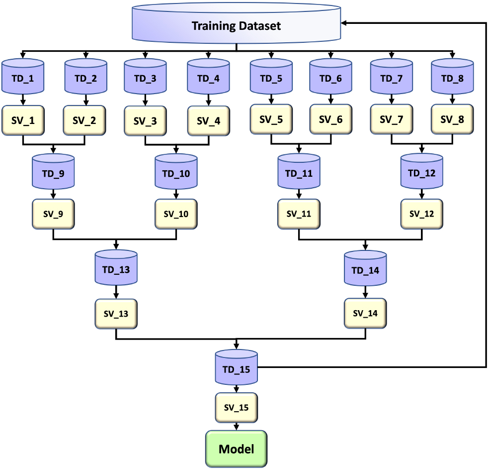

In view of the deficiency of Cascade SVM, the DC-SVM algorithm is proposed in literature [29]. It divides the whole parallel process into two parts: divide and conquer. Specifically, it uses K-means to split the data, and adopts similar methods to merge the solutions through re-clustering and retraining, which improves the speed and accuracy of training. However, the disadvantage of DC-SVM is that, like the traditional Cascade SVM, at the last iteration, it operates a single SVM on the whole left training dataset. For the larger dataset, it is essentially quite slow and non-scalable.

Additionally, the CA-SVM [18] can avoid unnecessary communication, reduce overhead and accelerate the training process of SVM. Tao et al. [30] proposed a framework of large-scale kernel SVM by using BMMPGD (Budget Small Matching Parallel Gradient Descent) algorithm on Spark. Through experiments on Spark, they tested the time and accuracy of BMMPGD algorithm in different iterations and different data sizes. And compared the experimental results with SVMWithSGD (Support Vector Machines with Stochastic Gradient Descent) and LIBSVM [31]. Experimental results show that their algorithm has higher accuracy than SVMWithSGD, and has a very significant acceleration ratio compared with LIBSVM. Liu et al. [24] proposed multiple submodels parallel SVM (MSM-SVM) method on Spark to accelerate the training process of nonlinear SVM. Based on the SVM model theory, they introduced a clustering-based data segmentation method, so that the parallel training process and the approximate global solution have multiple local sub-models. And the experimental results show that the MSM-SVM performs well in both binary classification and multi-classification. It is also superior to SVM With MiniBatch SGD in Spark MLlib. In addition, Gonzalez-Lima et al. utilized Locality-Sensitive Hashing (LSH) for solving the optimization problem that the volume of support vector machines surge to a large extent for large data sets in high dimensions. LSH is enable to search for neighbors efficiently in high dimensional spaces [32].

Afterwards, the conecpt of parallelization is introduced to SVM and many new parallelized SVM algorithms are emerging. In the literature [33], a parallelized SVM algorithm is proposed. It can effectively reduce the size of dataset before the training process and recover effective data from the eliminated samples to accelerate SVM. Additionally, Xia et al. introdeuced the parllel grid into SVM, i.e., a parallel Grid-Search-based Support Vector Machine (GS-SVM). It provides an efficient methodology with Spark engine to search for passengers in a complex urban traffic network quickly [34]. Moreover, in literature [35], the accelerated SVM algorithm improves performance to 45%, memory usage to 15.41%, and execution time per accuracy to 41.3% compared to a linear support vector machine implemented from Tensorflow Lite. Additionally, more and more efforts are being made to improve the performance of SVM [36, 37, 38].

3. Background

3.1 Mathematical derivation of SVM

SVM algorithm has strong generalization and learning ability, and overcomes the shortcomings of traditional machine learning algorithms such as overfitting, dimension disaster and local minimum. SVM is suitable for the binary classification model normally [39]. Its basic model is a linear classifier defined in feature space with maximum spacing [40], which can transform the problem into a convex quadratic programming problem. Specifically, it is adopted to find the optimal classification hyperplane for two kinds of samples in the original space when the problem is linearly divisible. In the case of linear inseparability, the samples from the low-dimensional input space are mapped to the high-dimensional space by using a non-linear mapping and adding relaxation variables to make them linearly separable. Therefore, the optimal classification hyperplane can be found in high-dimensional space.

Additionally, the classification hyperplane also should maximize the distance of the edge hyperplane, i.e, the classified hyperplane with the maximum edge distance [41]. First, we define the objective function of hyperplane, as shown in Eq. (1) (Eqs (1)–(3.1) are referenced from article [42]). Then we solve the maximum edge distance with constraints, as shown in Eq. (3.1):

$\displaystyle h(x)=\omega x+b=0$ (1) $\displaystyle\min\frac{1}{2}\mid\mid\omega\mid\mid^{2}$ (2) $\displaystyle s.t.\quad y_{i}(\omega x_{i}+b)\geqslant 1,\quad i=1,\ldots n$

Furthermore, the maximum edge distance problem can be transformed into a simple dual problem by using Lagrange optimization method. The Lagrange function of convex quadratic programming is defined Eq. (3):

$\displaystyle L_{P}(\omega,b,\alpha)=\frac{1}{2}\mid\mid\omega\mid\mid^{2}-% \sum_{i=1}\alpha_{i}y_{i}(\omega x_{i}+b)+\sum_{i}\alpha_{i}$ (3)

Then calculate the minimal value of the problem $L_{P}$ , i.e., taking the derivative of $w$ and $b$ Eq. (3.1):

$\displaystyle\frac{\partial L_{p}}{\partial\omega}=\omega-\sum_{i}\alpha_{i}y_% {i}x_{i}=0\rightarrow\omega=\sum_{i}\alpha_{i}y_{i}x_{i}$ (4) $\displaystyle\frac{\partial L_{p}}{\partial b}=\sum_{i}\alpha_{i}y_{i}=0$

Afterwards, the corresponding dual problem $L_{D}$ is obtained by bringing $\alpha$ back to $L_{P}$ Eq. (5).

$\displaystyle L_{D}(\alpha)=\sum_{i}\alpha_{i}-\frac{1}{2}\sum_{i,j}\alpha_{i}% \alpha_{j}y_{i}y_{j}(x_{i})^{T}x_{j}$ (5)

KKT conditions met are shown in Eq. (3.1).

$\displaystyle\alpha_{i}\geqslant 0$ $\displaystyle\sum_{i}\alpha_{i}h(x_{i})=0$ (6) $\displaystyle h(x_{i})\leqslant 0$

Meanwhile, $L_{D}$ is also constrained by Eq. (7).

$\displaystyle\sum_{i}\alpha_{i}y_{i}=0$ (7)

Therefore, the original problem $L_{P}$ minimization of $\omega$ and $b$ is transformed into the dual problem $L_{D}$ maximization of $\alpha$ . And $L_{D}$ contains only the variable $\alpha$ . According to KKT condition, only the $\alpha_{i}$ corresponding to support vector $x_{s}$ is greater than 0, while the $\alpha_{i}$ corresponding to other data points $x_{i}$ are all 0. Therefore, only support vectors need to be considered in calculation Eq. (3.1).

$\displaystyle\omega=\sum_{i}\alpha_{i}y_{i}x_{i}=\sum_{s\in S}\alpha_{s}y_{s}x% _{s}$ (8) $\displaystyle b=y_{s}-\sum_{k\in S}\alpha_{k}y_{k}x_{k}^{T}x_{s}$

3.2 Advantages and disadvantages of SVM

The main advantages of SVM are shown below.

High-dimensional efficiency. In order to improve the efficiency of the algorithm in the high-dimensional space, the nonlinear mapping to the high-dimensional space can be replaced by the kernel function in the SVM training process [39].

Simple calculation. Compared with some traditional classification methods, SVM does not use the law of large numbers, probability measure and other more complex operation theorems, which greatly simplifies the calculation process.

Avoid dimensional disasters. The determinant of SVM training results is the global support vector, which is a small proportion of the sample dataset. Specifically, the spatial dimension of the dataset does not play a decisive role in the computational complexity of the algorithm. Only the size of the support vector set affects the complexity of the algorithm, which avoids the “dimension disaster” caused by too many dimensions.

Whereas, SVM has several disadvantages.

SVM is difficult to implement for large-scale training samples. This is because the SVM algorithm uses quadratic programming to obtain the support vectors, which involves the calculation of m-exponent matrix. Thus it will consume a lot of machine memory and operation time when the matrix exponent is large [9, 43].

The general SVM algorithms have a bad performance on multi-class classification [44, 45]. But there are several specified SVM algorithms support muli-class classification with specified methods, such as LibSVM.

The effect of SVM algorithm has a great relationship with the selection of kernel function, so it is often necessary to try a variety of kernel functions. Even if the Gaussian kernel function with better effect is selected, the appropriate $\gamma$ parameter should be adjusted and selected. On the other hand, the commonly used SVM theories all use a fixed penalty coefficient C. But the losses caused by the two types of errors, positive and negative samples, are different.

3.3 Spark

Spark is a general big data computing platform developed by UC Berkeley AMP Lab. And Spark is implemented by scala functional programming language, and provides APIs of Java, Python and other languages for developing applications [46, 47]. Spark is fully compatible with Hadoop’s original ecosystem, and uses HDFS as a distributed storage system. Meanwhile, Spark’s memory-based computing model overcomes the shortcomings of Hadoop MapReduce in iterative computation and interactive data analysis. Spark puts the computational intermediate data in memory instead of disk, which has high efficiency of iterative operation. Moreover, Spark supports distributed parallel computing of DAG graph, which reduces the landing of data in the iterative process and improves the processing efficiency. The architecture of Spark is shown in Fig. 2, which mainly consists of four components: Cluster Manager, Worker Node, Driver and Executor [48].

Cluster Manager: The master node in standalone mode and the resource manager in YARN mode.

Worker node: The worker node is a slave node in Standalone mode and a NodeManager in YARN mode.

Driver: Running the main function of Application.

Executor: A process runs on a worker node for an Application.

Figure 2.

Spark architecture.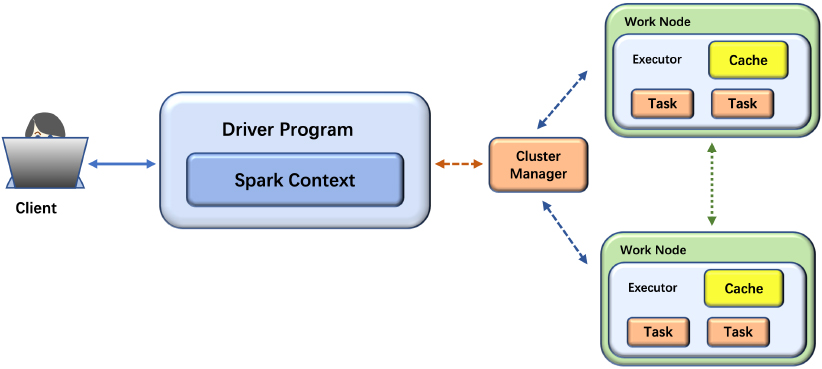

The Resilient Distributed Dataset (RDD) is the core of Spark’s data storage [49]. It allows efficient sharing of data in iterative computation. In addition, RDD is an essential metadata structure that provides a highly limited memory model. It records a set of read-only partition records and their logical structural mapping relationships. In Spark programming model, RDD is represented as an object, and is classified into two types, namely, transformations and actions. Transformations are inert operators, which generates new RDD after execution. Therefore, RDDs form an interdependent relationship with each other. In addition, action is the operator that actually triggers the execution of the program. It returns the public value type to the Driver program or exports the data to an external storage system.

Moreover, the dependency relationship of RDD is divided into wide dependency and narrow dependency. Narrow dependency means that the partition of child RDD only depends on one partition of parent RDD, which is a one-to-one relationship. While wide dependency means that each partition of child RDD depends on multiple partitions of parent RDD. Besides, RDD implements two fault-tolerant methods: recording conversion information and data checkpoint. Due to the high cost of data checkpoint operation and the large amount of network bandwidth required, RDD usually uses recording conversion information for fault tolerance by default to recover lost partitions. Whereas encountering wide dependency or too many conversion operations, checkpoints can be used for fault tolerance.

Additionally, in Spark, the repartition operator and the coalesce operator are two parallel operators. The difference between the two is that repartition is a special version of coalesce adding shuffle, which can reduce or increase the number of partitions. In this paper, the support vectors (SVs) obtained by each node are redistributed by the repartition operator acoording the K-means center points, i.e., shuffle. However, in the process of shuffle by the repartition operator, a random number generated by the HashPartitioner is used as the key, which leads to the imbalance of data on each node. Additionally, there is potential the problem that the local SV union of each node does not represent the global SV, resulting in inaccurate and low accuracy of the classification hyperplane. Therefore, the PB-SVM we proposed solves the problems of data skew and unbalanced SVs of each node effectively.

4. The design of PB-SVM

Figure 3.

Overall flow chart of PB-SVM algorithm.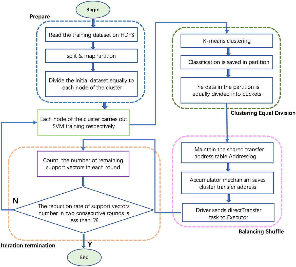

The PB-SVM algorithm is mainly divided into three stages, i.e., Clustering Equal Division, Balancing Shuffle, Iteration Termination. The overall flow chart of PB-SVM is shown in Fig. 3. We implement the PB-SVM in a real Hadoop YARN cluster [50]. Hadoop YARN is a distributed cluster, the SVM training is carried out on every node in the cluster respectively. In the preparation stage, the training dataset are downloaded from HDFS (Hadoop Distributed File System). Then, the dataset is divided into N equal parts by using the split and the mapPartition operators, and every part is sent to different Hadoop nodes by using HashPartition. Indeed, each Hadoop node has roughly the same amount of data, which is beneficial for the next steps to achieve data balance. Finally, the training will be terminated when appropriate termination requirements are met.

4.1 Clustering equal division

First of all, this stage is based on the Cascade SVM algorithm, starting from the parallel idea of data block and divide-and-conquer [51, 52]. The hierarchical SVM training model merges the independent SVM after each iteration, resulting in more and more idle nodes in the cluster and the total time of iterative training is longer. To slove this problem, we restructure the training hierarchy and merging strategy.

Figure 4.

Clustering equal division.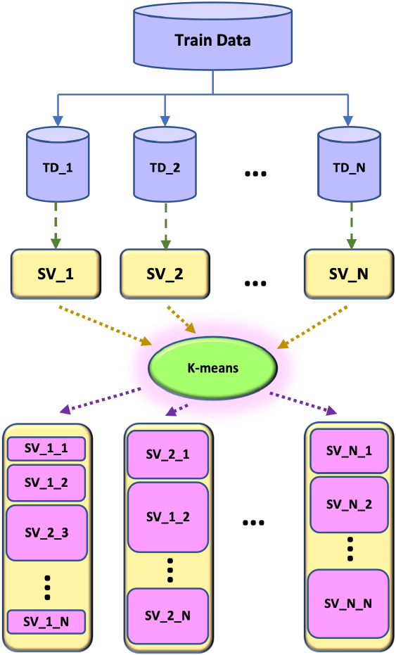

Indeed, the training structure is adjusted to single-level, as shown in Fig. 4. The adjusted structure is equivalent to each layer being the same in each iteration (Fig. 4). Specifically, after each iteration, the local support vectors of the two nodes are not merged into one node like the traditional Cascade SVM. First, we use the K-means clustering algorithm to quickly divide the local support vectors into N types (N is the number of cluster nodes), and put the N types of support vectors into their corresponding N partitions. Meanwhile, the number of support vectors of different nodes may be different, and the number of support vectors in different partitions of the same node may also be different. Next, the data of each partition is equally divided into N buckets. N also corresponds to the number of cluster nodes. After the equal division, the data is divided at bucket granularity, which is ready for the next shuffle phase.

4.1.1 K-means clustering description

The K-means algorithm in Mllib [53] uses a method of finding the cluster to which the sample point belongs, and then calculating the distance between the sample point and the center point. However, the K-means algorithm in this paper does a different job in the subsequent processing of clustering. First, the K-means algorithm is carried out on the first node of the cluster to complete SVM training to obtain N classification centers (N is the number of nodes in the cluster). Then these center points are saved in a list to be sent to the Driver side. Afterwards, the Driver uses specific broadcast mechanism to broadcast the information of the classification center to other nodes in the cluster. As shown in Fig. 5, the broadcast mechanism we utilize is implemented by Spark. The broadcast variable (classification center) can be shared and accessed from the cluster, but cannot be modified. They are created using the SparkContext.broadcast() method, which returns an object of type Broadcast. And the value can be any serializable object, which is able to be read by the executor using the Broadcast.value method. When the executor tries to read the broadcast variable, the executor will first check whether it has been loaded. If not, it requests broadcast variables from the Driver, one block at a time. This pull-based method avoids network congestion when the job is started.

Figure 5.

Broadcast the center list.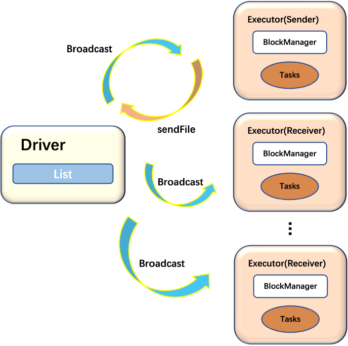

Additionally, since each node in the cluster performs SVM training in parallel, the order in which they complete their respective training is different. Therefore, we supplement for the broadcasting mechanism mentioned above. Specifically, the node that first completes the local SVM training will communicate with the Driver, informing it that it is the first node to complete the training. Then this node will become the Sender, and the other nodes will become Receiver. The purpose is to prevent the cluster from generating multiple senders, causing multiple copies of K-means central point information to be broadcasted. If there are multiple senders, it will cause multiple nodes to conduct K-means classification respectively. Therefore, the cluster centers obtained must be different, and each node in the subsequent process will be unrelated to each other. Thus losing the function of clustering.

Moreover, the list of the classification center point cannot be in the form of RDD. It needs to be instantiated and stored using the action operator. Specifically, it can be stored in memory or disk using the persist operator or saveAsTextFile operator. Because when the Driver side broadcasts, it cannot broadcast RDD, since RDD is an abstraction of data collection and does not store data itself.

4.1.2 Partition into equal buckets

Before training, we divide the dataset TD into N equally, where N is the number of cluster nodes. So the dataset TD_i on each node can be expressed as:

$\displaystyle\rm TD\_i=\left\{(X_{i},Y_{i})\right\},\quad i\in[1,N]$ (9)

Figure 6.

Partition into equal buckets.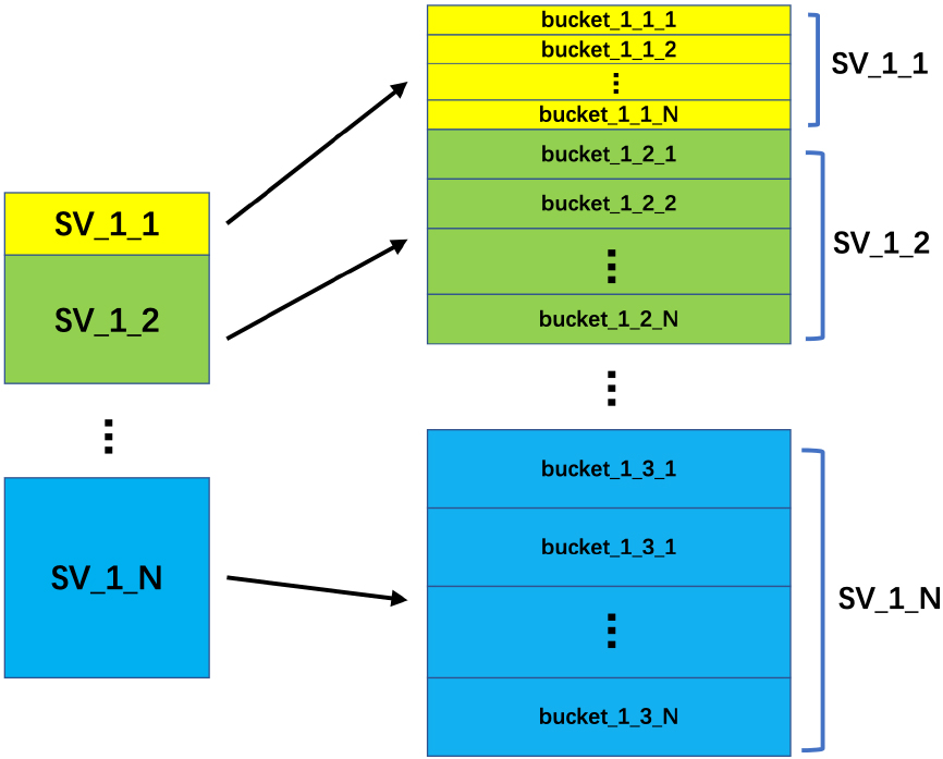

As shown in Fig. 6, the dataset TD_i on a node is divided into N partitions, where i in SV_i_j represents the node number, j represents the partition number (shown in Eq. (10)). And different partitions are represented by different colors. Similarly, each partition is equally divided into N buckets, and bucket_i_j_k represents the number of the bucket (k represents the number of the bucket in a partition).

$\displaystyle\rm SV\_i=\{SV\_i\_j\}_{j=1}^{N}$ (10)

Additionally, when the data in the partition SV_i_j is equally divided into buckets, the data is not randomly added to the buckets, but the incremental method is used. Therefore, according to the distance of each data point from the centroid, the data of every partition is added to the bucket with an increment of N, as shown in Fig. 7.

Figure 7.

Divide equally into buckets.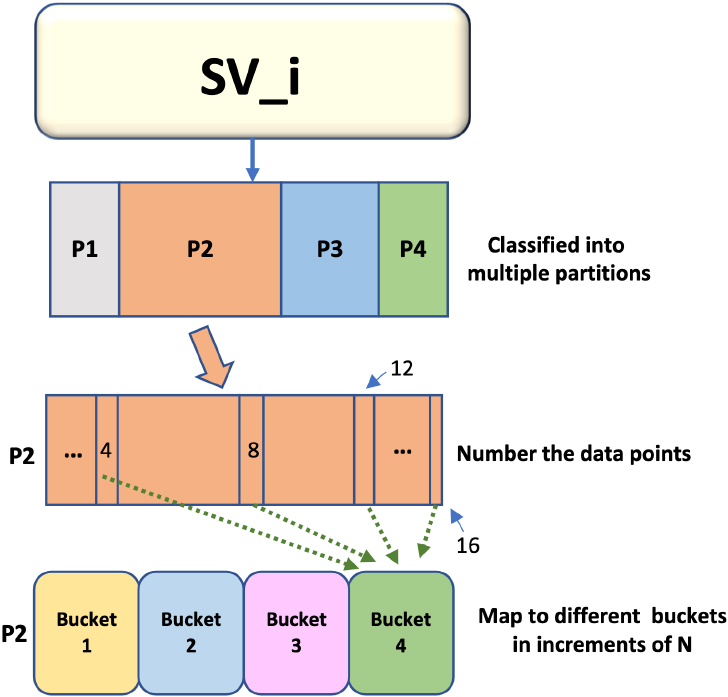

In this process, just like a hash table, the sort number of each data point takes the remainder of N (N is the number of cluster nodes), so that the data in each bucket is also evenly distributed. The even distribution of data also avoids the problem of heavily skewed data and unbalanced loads that exist with Cascade SVM. The whole process of Clustering Equal Division is shown in Algorithm 7.

[h] : Clustering Equal Division[1] TrainData

FilePath

N: the number of nodes in the cluster

TD_i: training dataset distributed at ith node

SV_i: support vectors obtained after ith node training

SV_i_j: partition j on node i

M: the number of support vectors on the partition

SV_c: ordered SVs set

bucket_i_j_k: bucket k in partition j on node i

AddressLog: record the address of the buckets

The addresses of the buckets to be transferred sc $=$ newSparkcontext(conf) TD $=$ sc.textFile(FilePath, N) TD_i $=$ TD.split().mapPartition() $i=1$ to $N$ SV_i $=$ train_svm(TD_i) $j=1$ to $N$ SV_i_j $=$ K-means(SV_i, K $=$ N) M $\leftarrow$ count(sv in SV_i_j) $\{SV_{c}\}_{c=1}^{M}$ $\leftarrow$ sort(sv in SV_i_j) $k=1$ to $N$ bucket_i_j_k $\leftarrow$ $\{SV_{c}\}_{c=k,k+N,k+2N\ldots}$ k $!=$ i AddressLog $\leftarrow$ bucket_i_j_k.address return AddressLog

Line 1–3: First, the SparkContext of Spark is created. Next, the training dataset is read into Spark cluster by using the operator textFile. And it is segmented and partitioned into N parts by using Spark’s own split and mapPartition operators.

Line 4–5: Spark cluster trains dataset on the nodes in parallel to obtain SV_i, i.e., local support vectors.

Line 7: The local support vectors on each node are classified into N classes by using the K-means clustering algorithm mentioned above. And SV_i_j represents the jth class on the ith node, i.e., a classification corresponds to a partition.

Line 8–9: The number of support vectors on each partition are saved in M. Then the data points are ordered from near to far according to the distance between them and the cluster center. Then they are saved in SV_c.

Line 11–14: The support vectors on each partition are divided into buckets, and the processing method is incremental addition. And the sorting number of data points is used to take the remainder of N. So every N-1 data points are added to the same bucket. Additionally, they are judged whether the current k is equal to i. If not, add the address of bucket_i_j_k to the AddressLog, i.e. this bucket should be transferred to other nodes.

Line 18: Finally, the for loop ends, and the returned AddressLog is the address set of the bucket to be transferred to other nodes.

4.2 Balancing shuffle

At this stage, based on the underlying source code of Spark’s repartition operator and the Spark Shuffle process, we develope an operator called directTransfer to transfer data to achieve Balancing Shuffle.

4.2.1 Transfer operator directTransfer

The AddressLog mentioned in Algorithm 7 is a shared file. But in a cluster environment, the shared variables are unable to be modified directly by executor on each node and globally visible. Here we need to utilize the accumulator technology supported by Spark. It provides a simple syntax to aggregate the values in the worker node into the Driver program. Spark supports user-defined accumulators that can be created by inheriting AccumulatorParam class. In Scala, although the data types of accumulated results and accumulated elements may be inconsistent, Spark provides a more general interface SparkContext.cumulative to accumulate data.

The directTransfer operates on each data block mapped by AddressLog. And there are two parameters required to be passed, i.e. the address of the transferred data block bucket SV_i_j_k and the destination address SV_k_j to which it needs to be transferred. The underlying layer of directTransfer operator calls the uploadBlock method of Nettyblocktransferserver service to upload files to remote Executor, which actually uses netty service created in Nettyblocktransferserver.

4.2.2 Implementation of balancing shuffle

The entire Balancing Shuffle process is shown in Fig. 8. After the Clustering Equal Division stage, the local support vectors have been evenly divided into buckets of different partitions. Then the directTransfer operator is used to transfer specific buckets to specific partitions of other nodes.

Figure 8.

Balancing shuffle.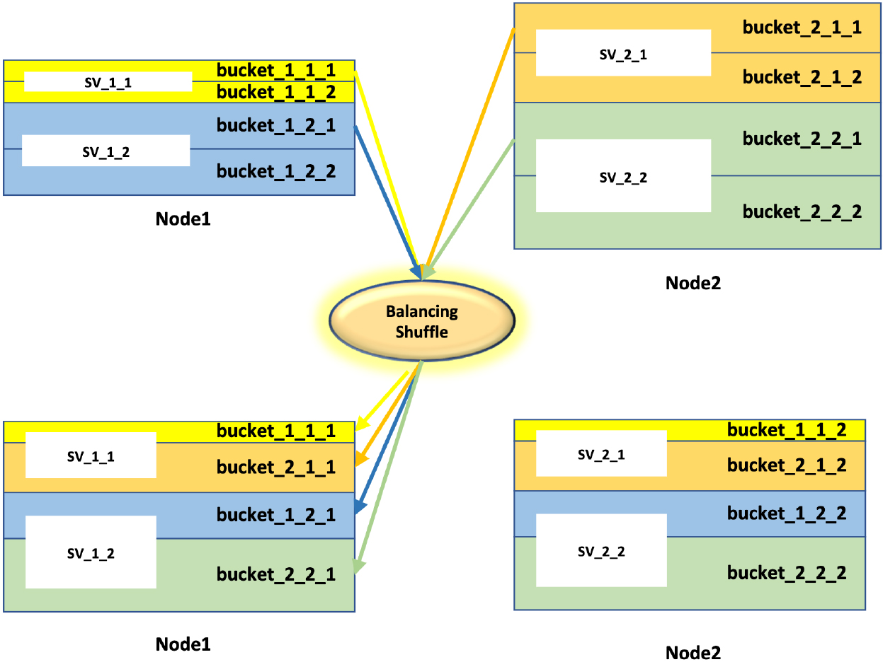

In the Fig. 8, we takes two nodes as an example. Each node is divided into two categories after the above K-means clustering algorithm, namely two partitions SV_i_1 and SV_i_2 (i is the node number). As shown in the Fig. 8, after different nodes train SVM respectively, the number of support vectors of every node are also different, which are represented by blocks with different colors and sizes in the figure. Specifically, during the operation of the directTransfer operator, as shown by the blue arrow in the figure, bucket_1_2_1 will be transferred to the partition of SV_1_2. Consequently, bucket_i_j_k will be transfer to the new partition with number i of the node with number k. In this way, the number of support vectors on each node is equivalent. This ensures data balance and avoids the problem of data skew. The entire Balancing Shuffle process is shown in Algorithm 8.

[h] : Balancing Shuffle[1]

AddressLog: the addresses of the buckets to be transferred

transfer_i: address record file of node i

transfer_i_j: address record file of j partition on node i

bucket_i_j_k: bucket k in partition j on node i

SV_k_j: partition j on node k balanced SVs $i=1$ to $N$ transfer_i $\leftarrow$ writeFile(AddressLog, i) $j=1$ to $N$ transfer_i_j $\leftarrow$ writeFile(transfer_i, j) turn transfer_i_j into a two-dimensional array $k=1$ to $N$ bucket_i_j_k $\leftarrow$ transfer_i_j[k][0] SV_k_j $\leftarrow$ transfer_i_j[k][1] directTransfer(bucket_i_j_k, SV_k_j)

Line 2: Write the information about node i in AddressLog obtained by Clustering Equal Division into transfer_i.

Line 4–5: Write the information about partition j in transfer_i into transfer_i_j and convert it into a two-dimensional array.

Line 6–10: Use the for loop to transfer the first value of each line in transfer_i_j to bucket_i_j_k (i.e., the buckets needed to transfer) and the second value to SV_k_j (i.e., the destination that the bucket transfer to). The directTransfer is a directional transfer operator written by us. The first parameter is the starting address, and the second parameter is the destination address. It is used to directionally send the data to the designated partition.

4.3 Iteration termination

The defects of the Cascade SVM algorithm have been mentioned above. With the increase of iterations, the number of non-support vectors that can be eliminated becomes less and less, and the training time becomes longer. Moreover, the more SVMs merged, the more idle nodes, resulting in a waste of resources. To solve this problem, it is necessary to judge the training end time of Cascade SVM and remove some iterations with low training efficiency. And the training efficiency of each iteration is quantitatively evaluated by parameters. When the training efficiency is reduced to a certain extent, subsequent iterations will not be required, and the final global training can be directly skipped to improve the overall efficiency of the algorithm.

In the Clustering Equal Division stage, we save the number of support vectors in each partition after clustering in the variable M (in Algorithm 7). Thus we can get the quantity of support vectors retained after a round of iteration. The optimization scheme proposed in this paper is to introduce a new parameter t, which is used to express the ratio of the number of support vectors of two adjacent iteratios. Specifically, t equals the ratio of the total number of support vectors in round i to the total number of support vectors in round i-1. Regarding the setting of the t benchmark, a small value of the t benchmark will result in too many iterations removed, a larger final number of global support vectors and a longer training time for the final iteration. Whereas, if the benchmark of t is large, the iteration reduction is not significant. We set a range of t from 0.8 to 0.99 for our experiments. For the five datasets used in this paper, 0.95 is the most appropriate standard value for the t parameter. Since the scale and type of datasets used in the experiment are different, 0.95 is a relatively common benchmark value, which is suitable for most datasets. In actual calculations, the reference value can be adjusted in a small range according to the specific dataset.

In Algorithm 4.3, whole_i represents the total number of support vectors after the ith iteration. And boolean variables is_termination1 and is_termination2 are set to determine whether the iteration is over, and their initial values are both false. When $\textit{whole\_i}+1$ /whole_i $\geqslant$ 0.95 appears for the first time, only is_termination1 is set to true. If the next round of $\textit{whole\_i}+2$ / $\textit{whole\_i}+1$ $\geqslant$ 0.95, is_termination2 is set to true, and the iteration ends. Otherwise, is_termination1 returns to false. The purpose of this is to prevent the occurrence of accidental situations.

[htbp] : Iteration termination[1]

$M_{j}$ value on each partition

whole: total number of support vectors in a certain round

whole_former: total number of support vectors in previous round

is_termination1: end judger 1

is_termination2: end judger 2

GlobalSVs whole $\leftarrow$ sum( $M_{j}$ ) is_termination1 $\leftarrow$ false, is_termination2 $\leftarrow$ false Does not meet the shutdown conditions t $=$ whole/whole_former t $>=$ 0.95 is_termination1 $==$ true is_termination2 $\leftarrow$ true return collect(SVs) is_termination1 $\leftarrow$ true whole_former $\leftarrow$ whole is_termination1 $\leftarrow$ false

5. Experiment

We compared PB-SVM with Cascade SVM, the latest LIBSVM and MLlib-SVM with several datasets. We conducted our experiments in a cluster of eight servers in Alibaba Cloud environment. The cluster includes a master node and seven worker nodes, and each node is configured with Spark 2.4.0, Hadoop 2.6.0 and JDK 1.8.0_172. The dataset used in this experiment is shown in Table 1. The ratio of training set to test set for all datasets is 8:2. We tested each algorithm 10 times to get an average of the results.

Table 1
Dataset info

Dataset	Source	Samples	Features	Classes
Mnist	YL98a	70,000	780	10
Ijcnnl	DP01a	49,990	22	2
Shuttle	Statlog	58,000	9	7
Letter	Statlog	20,000	15	26
Covtype	UCI	581,012	54	27

5.1 Comparison of binary classification results

Since the current SVM method in MLlib only supports binary-classification, the experiment is conducted first with the stand-alone LIBSVM, the SVMWithSGD [54] method in MLlib (MLlib-SVM), Cascade SVM on Spark. And we select the ijcnnl and covtype datasets for evaluating. The results are shown in Table 2 and Fig. 9. It is clear that the accuracy of the PB-SVM algorithm proposed in this paper is very close to LIBSVM, and is significantly better than MLlib-SVM and Cascade SVM on Spark. As shown by the time in Table 2, PB-SVM has the shortest computing time on these two datasets.

Table 2
Comparison result of binary classification

Dataset	Ijcnnl		Covtype
Algorithm	Time (s)	Accuracy	Time (s)	Accuracy
LIBSVM	102	0.9819	29874	0.9673
MLlib-SVM	42	0.9292	485	0.8943
Cascade SVM on Spark	58	0.9346	1202	0.8821
PB-SVM	28	0.9808	296	0.9659

Figure 9.

Comparison of accuracy of binary classification.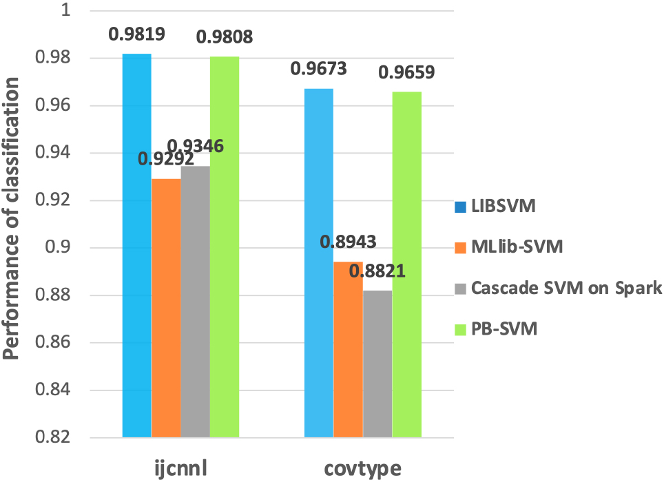

Figure 10 is a comparison of the training time of the ijcnnl and covtype datasets. As shown in Fig. 10a and b, although the LIBSVM has the highest accuracy among these four algorithms, it’s training time significantly longer than the other three methods on these two datasets. By contrast, PB-SVM consumes the least time and has the similar accuracy with LIBSVM. Moreover, for the dataset covtype, PB-SVM is nearly 100 times faster than LIBSVM, and 1.6 times and 4.1 times faster than MLlib-SVM and Cascade SVM on Spark, respectively. And the accuracy of PB-SVM increased by 7.16% and 8.38% than MLlib-SVM and Cascade SVM on Spark, respectively. In order to elaborate Fig. 10b, we compared the training time of three other methods except LIBSVM in Fig. 10c.

Figure 10.

Comparison of training time in binary classification.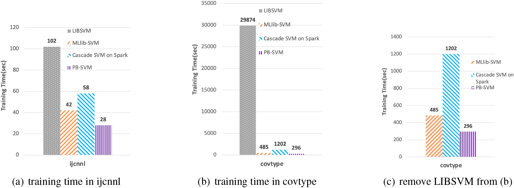

5.2 Comparison of multiple classification results

We conducted multi-classification experiments on four datasets of mnist, shuttle, letter and covtype. We implemented the PB-SVM with the RBF Gaussian kernel function [24], and the penalty parameter C and $\gamma$ are set to 2 and 0.09 respectively. As shown in Table 3 and Fig. 11, the PB-SVM algorithm proposed in this paper achieves good performance on the four datasets. The accuracy of PB-SVM is better than LIBSVM on the mnist, letter and covtype datasets, and very close to LIBSVM on the shuttle dataset. Figure 12 shows the time comparison of multi-class training on these four datasets. Obviously, PB-SVM spends the least time on these four different datasets. Compared with LIBSVM, the training speed of PB-SVM on covtype dataset is 80 times than it. And PB-SVM is faster than Cascade SVM on Spark on covtype 19 times, and the accuracy is improved by 18.3%.

Consequently, the above results give us some implications that the clustering partition equalization and balanced shuffling can better ensure the data balance on each node and avoid the accuracy degradation caused by data skew. Meanwhile, PB-SVM offers prominent performance in terms of runtime, which verifies the effectiveness of the PB-SVM algorithm compared by the Cascade SVM. This is because PB-SVM cancel the process of nodes merging. And all the nodes can be utilized in every iteration, which makes full use of the cluster’s resources.

Table 3
Datasets info

Dataset	Mnist		Shuttle		Letter		Covtype
Method	Time (s)	Accuracy	Time (s)	Accuracy	Time (s)	Accuracy	Time (s)	Accuracy
LIBSVM	485	0.9732	47	0.9915	82	0.9481	45192	0.9511
Cascade SVM on Spark	129	0.9662	29	0.8763	36	0.9217	10843	0.7706
PB-SVM	72	0.9746	13	0.9908	15	0.9503	563	0.9532

Figure 11.

Accuracy comparison of multiple classifications.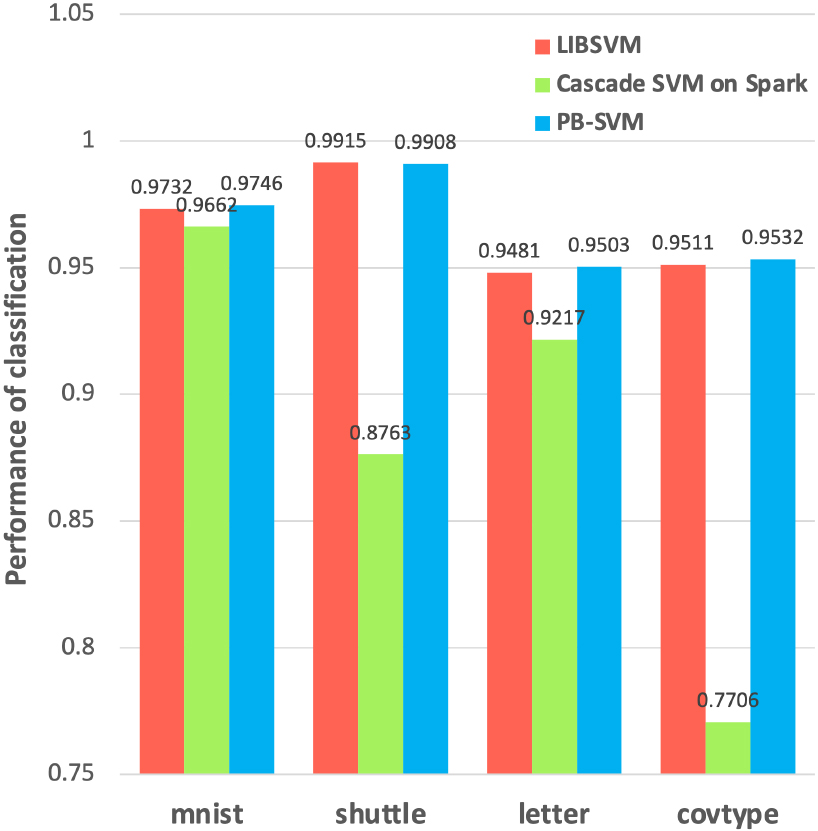

Figure 12.

Comparison of training time in multiple classifications.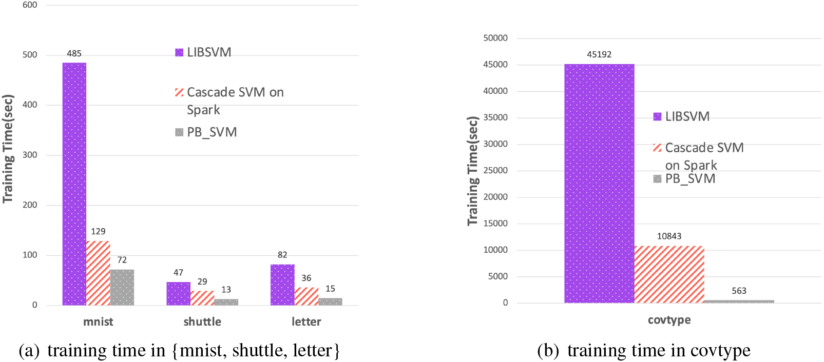

5.3 Comparison of other related results

We randomly selected six sub-datasets from the dataset mnist, and evaluated PB-SVM, LIBSVM algorithm and Cascade SVM on Spark algorithm respectively. We conducted six iterations for every kind of algorithm, and each iteration with 10,000 data points for testing. Figure 13 records the running time of these three algorithms. At the begining, when the number of data points is small, the training time of single-machine LIBSVM is close to the training time on PB-SVM and Cascade SVM on Spark. This is because the cluster computing needs to initialize related tasks, including creating jobs, allocating resources, scheduling tasks, tasks’ communication, data shuffle, etc. Indeed, if the volume of the dataset is small, the advantage of the cluster’s computing is not obvious. Furthermore, as the sample size increases, the advantages of the two parallel algorithms PB-SVM and Cascade SVM on Spark become more and more obvious. Due to the large amount of data, each node in the cluster can perform the training task in parallel, making full use of the advantages of parallel computing. Compared with Cascade SVM on Spark, the PB-SVM we proposed requires less training time under different data scales, which is consistent with the above conclusion. The PB-SVM algorithm can better improve parallel efficiency and reduce overhead.

Figure 13.

Training time of different data amounts.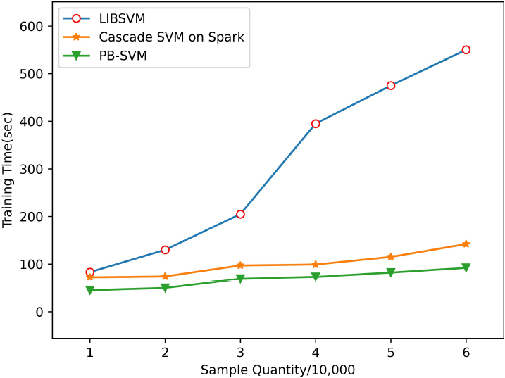

Figure 14.

Comparison of global SVs between PB-SVM and cascade SVM on spark.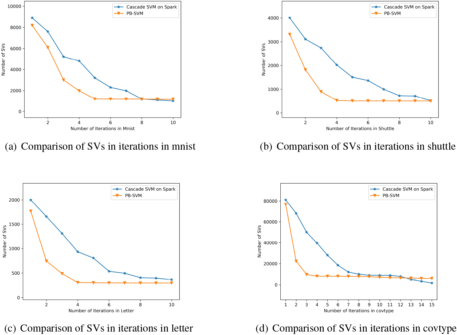

Finally, we compared the difference in the retention number of support vectors (i.e., the global support vectors) between Cascade SVM and PB-SVM on Spark on four datasets. In addition, since these two algorithms need to go through all iterations to find all truly global support vectors, so this experiment does not include the iteration termination part. The Fig. 14 shows that the training speed of PB-SVM is faster than Cascade SVM on Spark with the same dataset. And in the first few rounds of iterations, a large number of non-support vectors are quickly eliminated. As can be seen from the figure, the curve of PB-SVM is steeper in the first half and has a larger slope. And after about five rounds of training on these four datasets, the curve of PB-SVM tends to be flat, indicating that the final global support vectors have been basically found. Whereas, the Cascade SVM on Spark algorithm still retains a considerable number of non-support vectors. After the PB-SVM curve tends to converge, there are very few non-support vectors eliminated in the subsequent iterations. This also verifies the effectiveness of the iteration termination in Algorithm 4.3, which can end unnecessary iteration training early. Thus saving time and improving performance. Moreover, as shown in Fig. 14a, after the 9th and 10th rounds of training, the number of support vectors in PB-SVM is more than that in Cascade SVM. Thus the final accuracy verification also shows that Cascade SVM on Spark erroneously eliminated part of the global support vectors.

6. Conclusion

As an excellent machine learning algorithm, SVM has been developed for more than 20 years, and it plays a key role in many fields, such as data mining, text classification, face recognition and etc. The combination of Spark and SVM can take full advantage of Spark’s parallel computing to speed up the SVM training speed. Based on these, we propose a parallel equalization SVM algorithm based on Spark called PB-SVM. First of all, unlike the traditional Cascade SVM, the PB-SVM algorithm cancels the nodes emerging (two by two) after each iteration. PB-SVM adopts the same structure with all nodes in each iteration. Thus all the nodes in the cluster are able to participate in model training, which improves the resource utilization of the whole cluster. Additionally, the specified K-means clustering algorithm and broadcast mechanism in this paper is used to classify, partition and broadcast the data of nodes in the cluster. According to the classification results, points in the partition are divided into N buckets in an increasing way according to the distance from the center point. So the data in each bucket of the same partition is almost balanced in quantity and kind. Then we use the specific communication mechanism to send the support vectors of N-1 buckets to new partitions of other nodes to realize data balance for the subsequent iterations. After several rounds of iterative training, the set of support vectors are the global support vectors.

Moreover, we implement PB-SVM with different datasets and calculate the quantity of support vectors retained in each training round. After analysis, the benchmark value of the iterative termination algorithm is obtained, and the algorithm jumps out of iterative training when the number of support vectors tends to converg. Thus the training can be finished as soon as possible and the time can be shortened without losing the support vectors. Experimental results show that the PB-SVM algorithm we proposed consumes less training time but can get higher accuracy in the case of two-class and multi-class. In addition, it is superior to Cascade SVM on Spark and MLlib-SVM in training speed and accuracy. Our experimental results show that in the two-classification test on the dataset covtype, compared with MLlib-SVM and Cascade SVM on Spark, PB-SVM improves efficiency by 38.9% and 75.4%, and the accuracy is improved by 7.16% and 8.38%. Moreover, in the multi-classification test, compared with Cascade SVM on Spark on the dataset covtype, PB-SVM improves efficiency and accuracy by 94.8% and 18.26% respectively. In the further, we plan to reduce the communication overhead of PB-SVM, optimize it with parallel method at algorithm level, and apply PB-SVM algorithm to the actual industrial scenes.

Footnotes

Acknowledgments

This work was supported by the National Key R&D Program of China (No. 2020YFB0204603).

References

and Wang

, Deep Learning and Data Mining for Book Recommendation: Retrospect and Expectation, in: 2022 14th International Conference on Computer Research and Development (ICCRD), 2022, pp. 60–64. doi: 10.1109/ICCRD54409.2022.9730317.

Jaillet

Laurent

and Teisseire

, Sequential patterns for text categorization, Intelligent Data Analysis 10(3) (2006), 199–214.

Soni

A.N.

, Text Classification Feature extraction using SVM, International Journal of Innovative Research in Computer and Communication Engineering 7(7) (2019), 3563–3569.

Costa

Ortale

and Ritacco

, X-class: Associative classification of xml documents by structure, ACM Transactions on Information Systems (TOIS) 31(1) (2013), 1–40.

Saatci

and Town

, Cascaded classification of gender and facial expression using active appearance models, in: 7th International Conference on Automatic Face and Gesture Recognition (FGR06), 2006, pp. 393–398.

Huang

Yang

and Yang

, Financial distress prediction using SVM ensemble based on earnings manipulation and fuzzy integral, Intelligent Data Analysis 21(3) (2017), 617–636.

Boser

B.E.

Guyon

I.M.

and Vapnik

V.N.

, A training algorithm for optimal margin classifiers, in: Proceedings of the Fifth Annual Workshop on Computational Learning Theory, 1992, pp. 144–152.

Ihlayyel

H.A.

Sharef

N.M.

Nazri

M.Z.A.

et al., An enhanced feature representation based on linear regression model for stock market prediction, Intelligent Data Analysis 22(1) (2018), 45–76.

Zuo

Lin

Jia

and Zhang

, F-SVM: Combination of Feature Transformation and SVM Learning via Convex Relaxation, IEEE Transactions on Neural Networks and Learning Systems 29(11) (2018), 5185–5199. doi: 10.1109/TNNLS.2018.2791507.

10.

Hoi

S.C.

Jin

Zhu

and Lyu

M.R.

, Semisupervised SVM batch mode active learning with applications to image retrieval, ACM Transactions on Information Systems (TOIS) 27(3) (2009), 1–29.

11.

Chen

Wang

Z.J.

and Ji

, A Load-Balancing Divide-and-Conquer SVM Solver, ACM Trans. Embed. Comput. Syst. 16(3) (2017). doi: 10.1145/3005347.

12.

Lian

and Fan

, Divide-and-Conquer for Debiased l<sub>1</sub>-Norm Support Vector Machine in Ultra-High Dimensions, J. Mach. Learn. Res. 18(1) (2017), 6691–6716.

13.

Zhang

Duchi

and Wainwright

, Divide and Conquer Kernel Ridge Regression: A Distributed Algorithm with Minimax Optimal Rates 16(1) (2015), 3299–3340.

14.

Ang

H.H.

Gopalkrishnan

Hoi

S.C.H.

and Ng

W.K.

, Classification in P2P Networks with Cascade Support Vector Machines, ACM Trans. Knowl. Discov. Data 7(4) (2013). doi: 10.1145/2541268.2541273.

15.

Graf

H.P.

Cosatto

Bottou

Durdanovic

and Vapnik

, Parallel Support Vector Machines: The Cascade SVM, in: Advances in Neural Information Processing Systems, 2004.

16.

Cui

Wang

Tan

and Peng

, Multi-Modes Cascade SVMs: Fast Support Vector Machines in Distributed System, 2017, 443–450.

17.

Song

Liang

and Wang

, An accelerator for support vector machines based on the local geometrical information and data partition, International Journal of Machine Learning and Cybernetics 10(9) (2019), 2389–2400.

18.

You

Demmel

and Czechowski

, CA-SVM: Communication-Avoiding Support Vector Machines on Distributed Systems, in: 2015 IEEE International Parallel and Distributed Processing Symposium, 2015, pp. 847–859.

19.

Singh

Roy

and Mohan

C.K.

, DiP-SVM: Distribution preserving kernel support vector machine for big data, IEEE Transactions on Big Data 3(1) (2017), 79–90.

20.

Jin

Xie

and Cao

, A distributed SVM method based on the iterative MapReduce, in: Proceedings of the 2015 IEEE 9th International Conference on Semantic Computing (IEEE ICSC 2015), 2015, pp. 116–119. doi: 10.1109/ICOSC.2015.7050788.

21.

Sun

and Fox

, Study on parallel SVM based on MapReduce, in: International Conference on Parallel and Distributed Processing Techniques and Applications, 2012, pp. 16–19.

22.

Z.S. Li Tao Liu Xuechen, Parallelization of support vector machine training based on hybrid programming model, Computer Research and Development 52(5) (2015), 1098–1108.

23.

Wang

Xiao

and Long

, Research of intrusion detection algorithm based on parallel SVM on spark, in: 2017 7th IEEE International Conference on Electronics Information and Emergency Communication (ICEIEC), 2017, pp. 153–156. doi: 10.1109/ICEIEC.2017.8076533.

24.

Liu

Yang

and Guo

, Multiple submodels parallel support vector machine on spark, in: 2016 IEEE International Conference on Big Data (Big Data), 2016, pp. 945–950. doi: 10.1109/BigData.2016.7840691.

25.

Nguyen

T.D.

Nguyen

and Phung

, Distributed data augmented support vector machine on Spark, in: 2016 23rd International Conference on Pattern Recognition (ICPR), 2016, pp. 498–503. doi: 10.1109/ICPR.2016.7899683.

26.

Apache Spark, 2021, https://spark.apache.org/docs/latest/.

27.

Islam

M.T.

Karunasekera

and Buyya

, Performance and cost-efficient spark job scheduling based on deep reinforcement learning in cloud computing environments, IEEE Transactions on Parallel and Distributed Systems 33(7) (2022), 1695–1710. doi: 10.1109/TPDS.2021.3124670.

28.

HDFS, https://hadoop.apache.org/docs/stable/hadoop-project-dist/hadoop-hdfs/HdfsDesign.html.

29.

Hsieh

C.J.

and S

, A Divide-and-Conquer Solver for Kernel Support Vector Machines, in: International Conference on Machine Learning, 2013, pp. 566–574.

30.

Tao

and Lin

, Budgeted mini-batch parallel gradient descent for support vector machines on Spark, 2014, 945–950.

31.

Chang

C.-C.

and Lin

C.-J.

, Libsvm, ACM Transactions on Intelligent Systems and Technology 2 (2011), 1–27. doi: 10.1145/1961189.1961199.

32.

Gonzalez-Lima

M.D.

and Ludeña

C.C.

, Using Locality-Sensitive Hashing for SVM Classification of Large Data Sets, Mathematics 10(11) (2022), 1812.

33.

Kang

Xiao

Chen

and Li

, An Improved Parallel SVM Algorithm on Distributed System, in: 2020 International Conference on Cyber-Enabled Distributed Computing and Knowledge Discovery (CyberC), 2020, pp. 204–209. doi: 10.1109/CyberC49757.2020.00040.

34.

Xia

Zheng

Bai

Yan

and Li

, A parallel grid-search-based SVM optimization algorithm on Spark for passenger hotspot prediction, Multimedia Tools and Applications, 2022, 1–27.

35.

Chang

Kang

and Park

, Accelerated SVM Algorithm for Sensors Fusion-based Activity Classification in Lightweighted Edge Devices, in: 2022 IEEE International Conference on Consumer Electronics (ICCE), 2022, pp. 1–4. doi: 10.1109/ICCE53296.2022.9730557.

36.

Tan

Guo

Jiang

Zhou

Yuan

and Zhang

, A new semi-supervised algorithm combined with MCICA optimizing SVM for motion imagination EEG classification, Intelligent Data Analysis 25(4) (2021), 863–877.

37.

Chen

Tan

and Zhang

, An iterative self-training support vector machine algorithm in brain-computer interfaces, Intelligent Data Analysis 20(1) (2016), 67–82.

38.

Gong

Guo

and Yang

, Active learning support vector machines with low-rank transformation, Intelligent Data Analysis 22(4) (2018), 701–715.

39.

Alam

Kang

Pyun

J.-Y.

and Kwon

G.-R.

, Performance of classification based on PCA, linear SVM, and Multi-kernel SVM, in: 2016 Eighth International Conference on Ubiquitous and Future Networks (ICUFN), 2016, pp. 987–989. doi: 10.1109/ICUFN.2016.7536945.

40.

and Yang

, Linear regression-based efficient SVM learning for large-scale classification, IEEE Transactions on Neural Networks and Learning Systems 26(10) (2015), 2357–2369.

41.

Shivaswamy

P.K.

and Jebara

, Maximum relative margin and data-dependent regularization, Journal of Machine Learning Research 11(2) (2010).

42.

Cristianini

Shawe-Taylor

et al., An introduction to support vector machines and other kernel-based learning methods, Cambridge university press, 2000.

43.

Shen

Chen

Kang

Zhang

Yang

and Liu

, Evolving support vector machines using fruit fly optimization for medical data classification, Knowledge-Based Systems 96 (2016), 61–75.

44.

Sun

Guo

Liu

Jiang

and Wang

, Fast multi-label SVM training based on approximate extreme points, Intelligent Data Analysis 22(5) (2018), 1079–1099.

45.

Zhang

and Wang

, The OCS-SVM: An Objective-Cost-Sensitive SVM With Sample-Based Misclassification Cost Invariance, IEEE Access 7 (2019), 118931–118942. doi: 10.1109/ACCESS.2019.2933437.

46.

Scala on Apache Spark, 2021, https://spark.apache.org/docs/latest/api/scala/org/apache/spark/index.html.

47.

Gupta

Y.K.

and Kumari

, A Study of Big Data Analytics using Apache Spark with Python and Scala, in: 2020 3rd International Conference on Intelligent Sustainable Systems (ICISS), 2020, pp. 471–478. doi: 10.1109/ICISS49785.2020.9315863.

48.

Mostafaeipour

Jahangard Rafsanjani

Ahmadi

and Arockia Dhanraj

, Investigating the performance of Hadoop and Spark platforms on machine learning algorithms, The Journal of Supercomputing 77(2) (2021), 1273–1300.

49.

RDD programming-guide, 2021, https://spark.apache.org/docs/3.2.1/rdd-programming-guide.html.

50.

Architecture of YARN, https://hadoop.apache.org/docs/stable/hadoop-yarn/hadoop-yarn-site/YARN.html.

51.

Xue

and Zhang

, A divide-and-conquer genetic programming algorithm with ensembles for image classification, IEEE Transactions on Evolutionary Computation 25(6) (2021), 1148–1162.

52.

Wardeh

Blagrove

M.S.

Sharkey

K.J.

and Baylis

, Divide-and-conquer: Machine-learning integrates mammalian and viral traits with network features to predict virus-mammal associations, Nature Communications 12(1) (2021), 1–15.

53.

Meng

Bradley

Yavuz

Sparks

Venkataraman

Liu

Freeman

Tsai

Amde

Owen

Xin

Franklin

Zadeh

Zaharia

and Talwalkar

, MLlib: Machine Learning in Apache Spark, JMLR 17 (2015).

54.

Platt

, Fast Training of Support Vector Machines Using Sequential Minimal Optimization, Advances in Kernel Methods: Support Vector Learning, 1999, 185–208. ISBN 0-262-19416-3.

A parallel and balanced SVM algorithm on spark for data-intensive computing

Abstract

Keywords

1. Introduction

2. Related work

3.1 Mathematical derivation of SVM

3.3 Spark

4.2.1 Transfer operator directTransfer

4.2.2 Implementation of balancing shuffle

5. Experiment

Table 1 Dataset info

Table 2 Comparison result of binary classification

Table 3 Datasets info

Footnotes

Acknowledgments

References

Table 1
Dataset info

Table 2
Comparison result of binary classification

Table 3
Datasets info