
Abstract
Missing data is one of the challenges a researcher encounters while attempting to draw information from data. The first step in solving this issue is to have the data stage ready for processing. Much effort has been made in this area; removing instances with missing data is a popular method for handling missing data, but it has drawbacks, including bias. It will be impacted negatively on the results. How missing values are handled depends on several vectors, including data types, missing rates, and missing mechanisms. It covers missing data patterns as well as missing at random, missing at completely random, and missing not at random. Other suggestions include using numerous imputation techniques divided into various categories, such as statistical and machine learning methods. One strategy to improve a model’s output is to weight the feature values to better the performance of classification or regression approaches. This research developed a new imputation technique called correlation coefficient min-max weighted imputation (CCMMWI). It combines the correlation coefficient and min-max normalization techniques to balance the feature values. The proposed technique seeks to increase the contribution of features by considering how those elements relate to the desired functionality. We evaluated several established techniques to assess the findings, including statistical techniques, mean and EM imputation, and machine learning imputation techniques, including k-NNI, and MICE. The evaluation also used the imputation techniques CBRL, CBRC, and ExtraImpute. We use various sizes of datasets, missing rates, and random patterns. To compare the imputed datasets and original data, we finally provide the findings and assess them using the root mean squared error (RMSE), mean absolute error (MAE), and
Keywords
Introduction
In the field of data mining and machine learning, the data preprocessing stage is a critical step for preparing the data and addressing any difficulties present in the raw data. The issue of missing data is one of the most prevalent problems encountered when working with data [1]. The dataset’s quality is significant because when the dataset is incomplete, obtaining knowledge becomes a complicated task [2]. Therefore, dealing with this issue is placed in the preprocessing stage in data mining. Also, understanding the reasons for missing data is essential, such as questions not answered by respondents because they prefer to avoid answering or consider it unnecessary [3]. Deleting instances/variables with missing data is a known way to handle missing data, but this solution can cause issues, such as bias, and negatively affect the results [4]. Classical techniques that use the deletion strategy are listwise and pairwise. Listwise involves deleting any instances with at least one missing value. Meanwhile, the pairwise strategy means using all the available data and only discarding the missing value when using the mode [5]. Another approach is to use imputation methods. The primary goal of missing data imputation is to improve data quality by using observed data to estimate missing values and fill them in using statistical or machine learning methods [6, 7, 8]. Numerous studies on imputing missing values have found that filling in missing data improves data quality and increases the accuracy of model output [9]. The choice of imputation methods depends on various factors, such as data size, type of data, missing rate, and a missing mechanism, which refers to how the missing values occur. It includes missing at random, missing at completely random, and missing not at random. Statistical methods include mean, median, and mode strategies that predict the methods based on observed values for each feature. Other imputation strategies are based on machine learning algorithms where the observed feature values are used to train the model and then predict the missing values. Techniques such as k-NN, SVM, and regression have been proposed to address the missing data problem. Feature normalization is a crucial step that adjusts the range of values to ensure that each feature contributes equally to the ML process, preventing any single feature from exerting undue influence solely due to its magnitude [10, 11]. The min-max method scales the values of each feature to lie between 0 and 1. On the other hand, the z-score method uses the mean and standard deviation to rescale the data, resulting in features with a mean of zero and unit variance. Many studies have explored the various effects of standardization methods on data to improve model performance [12, 13]. Ahsan, et al. [14] reported that no single normalization method can be considered the best, while Sinsomboonthong [15], Henderi, et al. [16], Raju, et al. [17] obtained good results using min-max scaling (0,1) compared to other methods. However, in the literature, several factors play a significant role in choosing the appropriate normalization method, such as the type of data and the specific application. Pires, et al. [9] studied how the imputation of missing data improves human activity monitoring accuracy using k-NN. The researchers found that imputation of missing values and normalization of the data increase the accuracy rate and improve the classification results. Benhar, et al. [18] have studied the impact of preprocessing methods on the classification methods used for heart disease data. One of the preprocessing impacts was handling missing data, while the other was the impact of normalization methods on the classification accuracy. This study aims to propose a numeric missing data imputation method called correlation coefficient min-max weighted imputation (CCMMWI) that weighs the values of the features using the correlation coefficient and min-max normalization method. The following section will discuss missing value issues, such as the missingness mechanism, missing patterns, and missing models. In Section 2, we will illustrate all the imputation methods used in this paper and how those algorithms work. In Section 3, we will explain the criteria used in this work and then show the results and how we evaluated them. Section 4 will include the experimental analyses of the results. Section 5 will present the discussion, followed by the research conclusion in Section 6.
Related work
Missing data has many mechanisms of missingness depending on how the values are missing. It is crucial to comprehend why values are missing [19]. Three types of missing data are: (i) missing completely at random (MCAR), where the data are missing entirely at random, meaning there are no dependencies on the missingness probability related to the missing values and the rest of the values [4]; (ii) missing at random, if the missing value only depends on the observed values [20]; and (iii) missing not at random, where the missing values’ mechanism may depend on other variables but also on the missing value itself [4, 20]. The missing data patterns include univariate and multivariate. The univariate pattern occurs when one variable has missing values; if more than one variable has missing values, it is called multivariate missing values. The missing pattern is called monotone when the variable has no observed values after the first missing values of a variable. Otherwise, the missing pattern is called non-monotone or general. The monotone pattern usually occurs in longitudinal data, where the data are collected from the same participants over the time of the study. A pattern of missing data is considered connected if any recorded data point can be accessed from any other recorded data point by a series of horizontal or vertical moves [21]. If the dataset’s missing values are distributed randomly in both instances and variables, it is called an arbitrary pattern [22]. The missing data pattern type is shown in Fig. 1.
Missing data percentage categories [25]
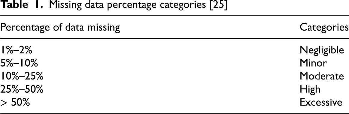
Missing data percentage categories [25]
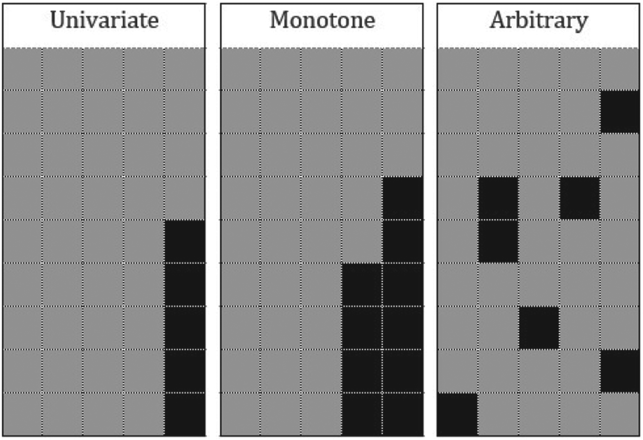
Missing data pattern (gray is observed, and black is missing).
The missing model is defined based on how the ratio of missing values is distributed among the features in the dataset. Two missing models exist: the uniformly distributed (UD) model and the overall model. In the UD model, the percentage of missing values is the same for each feature. In contrast, the overall model refers to when the proportion of missing values in each feature has a different value [23, 24]. The missing rate indicates how many values are missed in a dataset. Based on the missing percentage, the missing rate is categorized into five groups [25], as described in Table 1.
Listwise and pairwise deletion of features or instances containing missing values are the simplest ways to handle such values. Listwise deletion eliminates instances with missing values, while pairwise deletion uses all observed data in the analysis, excluding only the missing values [22, 26]. Imputations fall into two categories based on the features used in the imputation method. The first is intransitive, where imputation depends solely on the feature itself (e.g., mean mode) and not on other features. The second is transitive, where imputation depends on additional features, such as k-NN imputation, EM imputation, and regression method imputation [27]. Mean imputation, replacing missing values with the mean of observed values, is the most straightforward approach for dealing with missing data. Median and mode can also be used [28]. Mean imputation is acceptable if the missing rate is minor; otherwise, it may introduce bias [29, 30]. Another method is expectation–maximization (EM) [31]. The EM imputation method involves two steps: filling in the missing data in the expectation step and then re-optimizing the expectation step in the maximization step. This methodology performs well with massive missing data and a small sample [20]. k-NN (k nearest neighbors) is a widely used nonparametric method in machine learning for classifying data due to its simplicity, generality, and relatively high accuracy [32, 33]. The k-NN imputation (k-NNI) algorithm is proposed to handle incomplete data by averaging the k nearest neighbor values from all complete instances [34, 35]. Another nonparametric imputation method is missForest (MF), proposed by Stekhoven and Bühlmann [36], based on the random forest algorithm. It can handle both numeric and categorical variable types simultaneously and is computationally effective for high-dimensional data [37]. Buuren and Groothuis-Oudshoorn [38] proposed multivariate imputation by chained equations (MICE). MICE estimates incomplete datasets through three steps: data imputation, data analysis, and data pooling, employing one of the regression methods in the estimation step [39, 40]. In literature on data analysis, many researchers have explored the impact of missing data on machine learning model output and how to address this issue [6, 41, 42, 43]. Various imputing methods aim to deal with missing values using different techniques, where the primary goal is to increase data availability with good quality. As with many machine learning techniques, data with varying feature value scales must be addressed during preprocessing to prevent feature dominance. This issue has been resolved using one of the standardization and normalization techniques. Rahman and Islam [44] proposed FIMUS, emphasizing the correlation between features when estimating missing values. Sezer and Başeğmez [45] recommend a technique for missing value imputation based on dataset consistency-based feature selection. This technique identifies subsets of features with contradictory values (i.e., identical feature values but different class labels) using a multivariable measure rather than unary measures such as distance, information, or dependence. Alabadla, et al. [46] introduced the ExtraImpute method, using extremely randomized trees (extra trees) to address missing numeric values. CCMVI, proposed by [47], imputes missing values by computing the class center, similar to determining the cluster center in the k-means technique. Nugroho, et al. [48] extended this work by proposing a class-center imputation technique that evaluates the association of features with the imputation stage. Liu et al. [49] proposed a correlation-based hierarchical k-NNI method, utilizing the correlation coefficient among features to impute missing values. Sefidian and Daneshpour [50] introduced ten correlation-based imputation techniques that maximize the connection between a missing feature and the remaining features. These methods maximize the connection between a missing feature and the remaining features. Manna and Pati [51] proposed imputation, a technique based on the similarity of gene expression and correlation coefficient. Razavi-Far et al. [52] proposed two missing data imputation techniques: kEMI and kEMI+, with the essence based on the k-NN and EM methods, using k-NN for the pre-imputation stage and the EM algorithm for the posterior-imputation stage. Mostafa et al. [53] proposed two imputation methods based on the Bayesian ridge model: CBRL and CBRC. In CBRL, the priority of imputing missing values is determined by features with fewer missing values, while in CBRC, the priority is based on high correlation with the target. The authors also introduced another method named CBRG, which utilizes gain ratio feature selection to establish the priority of imputation [54]. Nonetheless, a significant limitation lies in the utilization of raw data for constructing the estimator model, assigning equal weight to all features, regardless of their varying importance. Furthermore, prior research suffers from the shortcoming of estimating the correlation coefficient based on a sub dataset containing non-missing values. This practice proves inadequate for capturing the intricate relationships between features, chiefly owing to the resultant dataset size reduction. The diminished number of samples can exert a substantial influence on the outcomes of the correlation matrix, particularly when handling datasets characterized by moderate to high missing rates. Moreover, while prior efforts have concentrated on prioritizing features with the highest correlation, there exists an unexplored opportunity to investigate the strength of feature relationships when constructing the model.
Proposed method
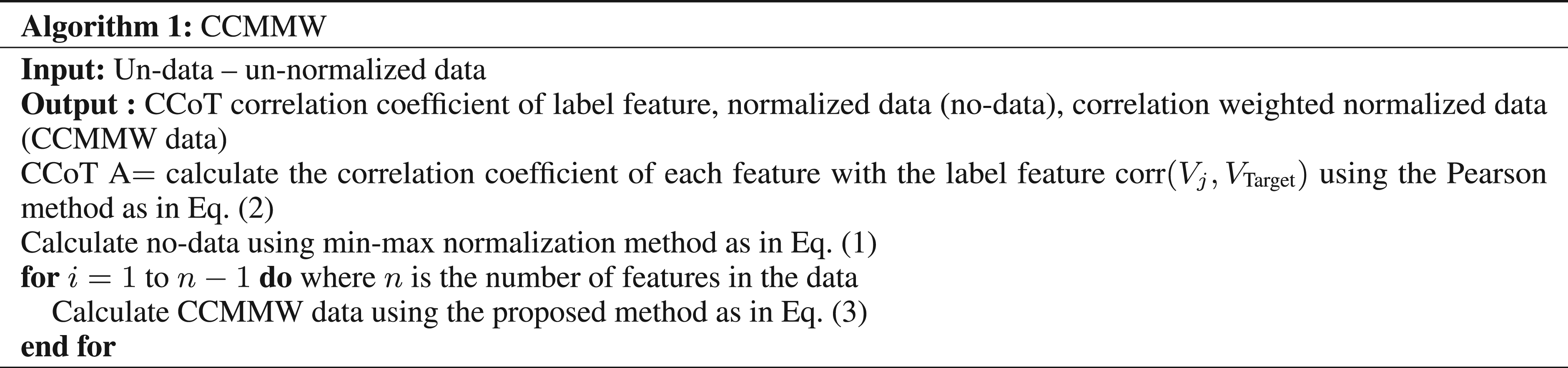
The proposed method is divided into two stages. The first stage is called CCMMW, which involves Weighting Feature values based on the Correlation Coefficient and Min-Max normalization method. CCMMW combines two preprocessing strategies to prepare the raw data and enhance its quality to achieve optimal output. First, it equalizes the contribution of features, and second, it weights the features based on the correlation among the dependent feature (label feature) and independent features (the rest of the features). Utilizing weighted feature values instead of raw data to build the estimator may enhance the model’s performance and reduce the error rate. The parameter C in CCMMW is proposed to adjust the new maximum value of features in the weighted values dataset. Algorithm 1 provides the pseudocode of CCMMW, and the primary mechanism of CCMMW is divided into three steps as follows:
Step 1: Normalize the original data to avoid any dominating features. For this step, the proposed method used min-max (0,1) to rescale feature values to a new range between 0 and 1. Equation (1) is used as the normalization method for this step.

Step 2: Calculate the correlation coefficient among the label feature and the independent features to use for weighting the values based on their correlation with the target. As in Eq. (2), The Pearson correlation coefficient has been chosen because of the numerical nature of the datasets involved in this study [55]. While normality is crucial for Pearson correlation, this study adopts a pragmatic approach by utilizing Pearson correlation without conducting individual normality tests for computational efficiency [56]. The decision is grounded in the acknowledgment that Pearson correlation is robust to deviations from normality, especially with large sample sizes. The analysis involves all available pairs in the datasets, recognizing the potential computational burden of testing each pair for normality. Future endeavors may include assessing individual pair normality and adjusting correlation methods accordingly, a step inspired by the overarching goal to understand and adapt to the intricacies of linear relationships between continuous variables [57, 58].

Step 3: Use Eq. (2) to weigh the values and create a new weighted dataset.

In the proposed work, we employed the CCMMW approach to impute missing values for each feature. After calculating the missing values across the entire dataset, features are arranged in descending order based on their correlation. We assume that the summation of the correlation for each feature serves as an indicator, where a higher correlation coefficient summation signifies a stronger correlation among features. An overview of the CCMMWI approach is provided before delving into each step of the proposed approach. As for the CCMMWI pseudocode as the Algorithm 2, assume that input
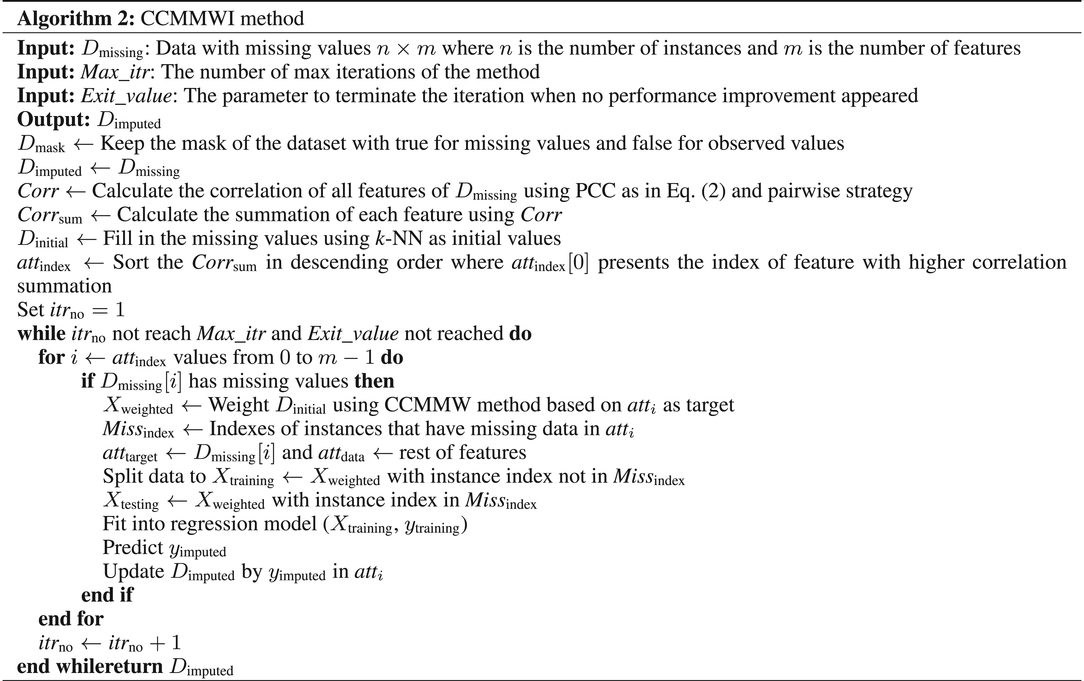

The flow of CCMMWI method.
Datasets
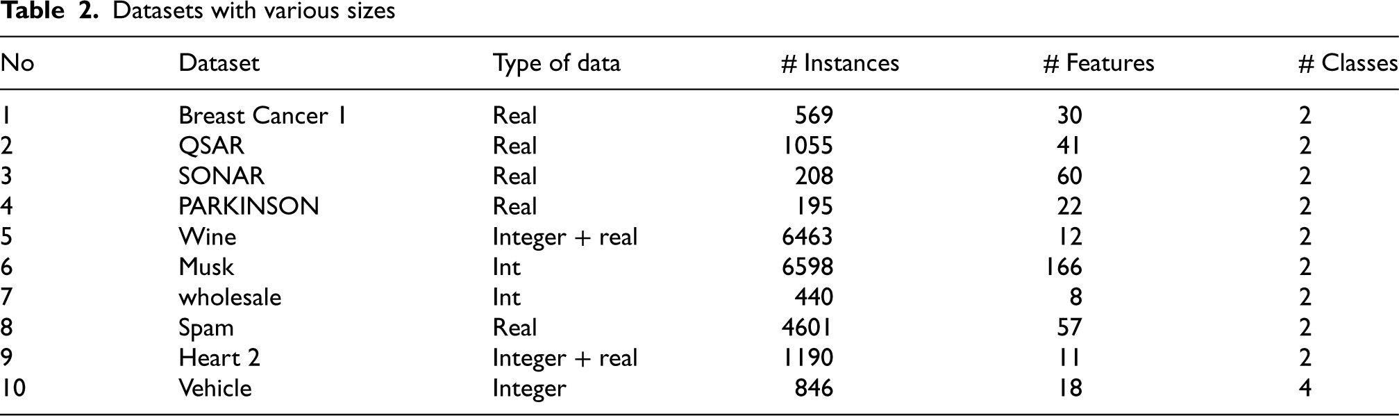
This study employed ten UCI datasets listed in Table 2 to assess the suggested imputation method’s effectiveness. Only numeric datasets are utilized, which are in integer and continuous values.
Datasets with various sizes
Datasets with various sizes
In this experiment, the proposed method is compared with MeanImp, k-NNI, EMI, and MICE imputation. Also, the evaluation section used three other imputation methods: CBRL, CBRC [53], and ExtraImpute [46]. The experiment steps are shown in Fig. 3.
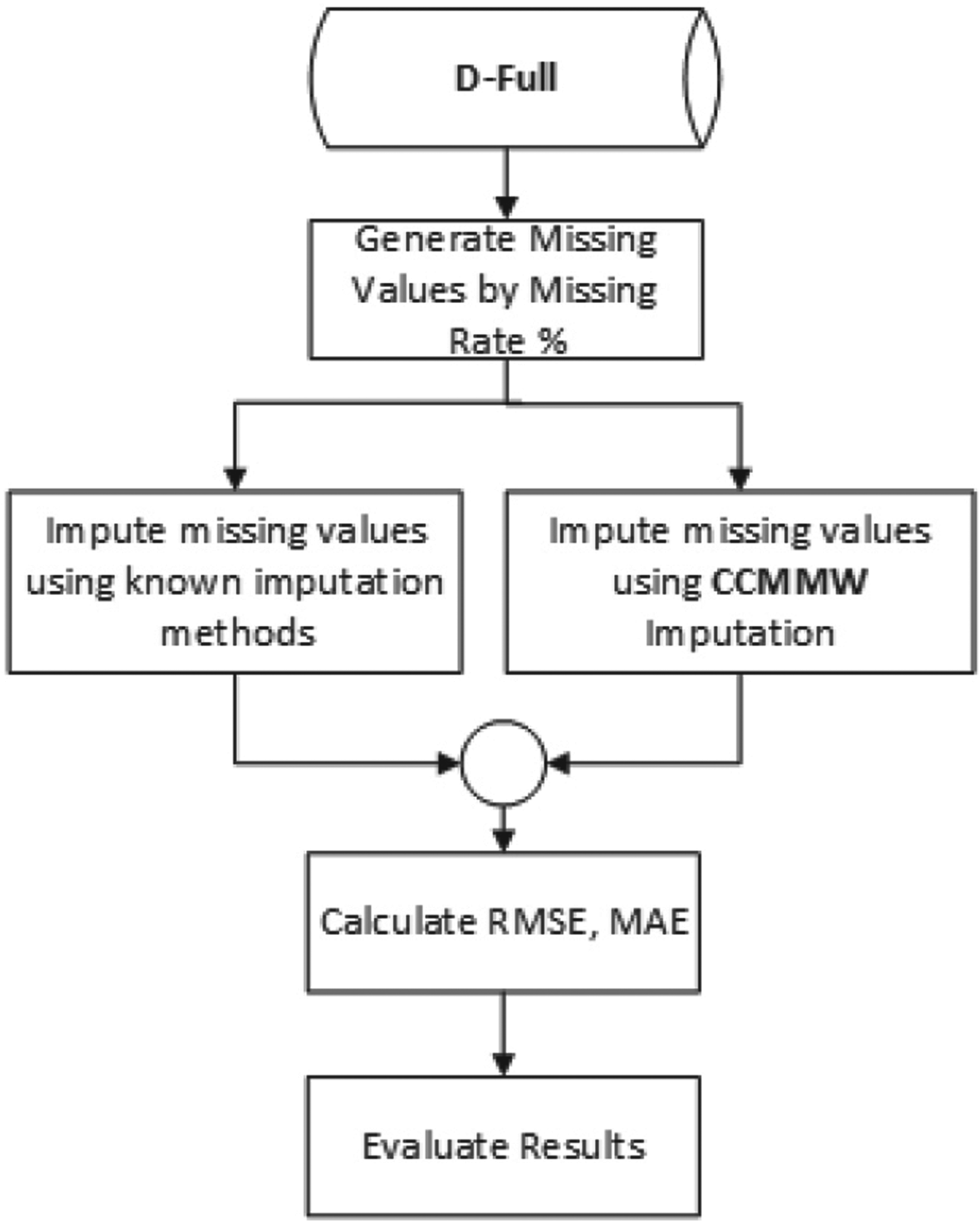
The experiment steps.
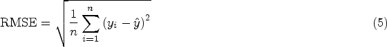
Based on Fig. 3, three evaluation metrics are considered to evaluate the generated imputed datasets. First, determine the error rate by using one error rate metric, to compare the original full dataset with the imputed dataset [59]. We evaluate the performance by calculating two statistics metrics, mean absolute error (MAE) and root mean squared error (RMSE), as in Eqs (4) and (5). MAE is the statistical error measure between paired observations that reflect the same phenomena. RMSE is the standard way in regression analysis to measure the quality of the model’s fit. Finally, the coefficient of determination (

In this experiment, all codes were written in Python 3.7. Jupyter (Anaconda 3), and SciKitLearn Library has been used to implement all the techniques. Finally, all experimental results were performed on numeric datasets. For all purposes, the result was evaluated by the RMSE, MAE, and
In this section, the results are categorized into two types. First, we present the outcomes of RMSE, MAE, and
Results based on RMSE
This section displays the results of applying various imputation techniques to datasets with varying levels of missing data, as measured by the RMSE. It reflects the discrepancy between the predicted and actual values in the data and is a commonly used metric for evaluating the performance of statistical models, including imputation techniques.
RMSE of each dataset
This section discusses the outcomes for each dataset where different missing rates are applied. The mean, EM, k-NNI, MICE, CBRL, CBRC, ExtraImpute (EXT.Imp), and CCMMWI techniques were used to impute the missing values.
Average RMSE based on datasets

Average RMSE based on datasets
As depicted in Table 3, CCMMWI yields a lower RMSE value in the Breast dataset compared to MICE, with both returning 0.0343. In QSAR, Sonar, Parkinson, Wine, Musk, and Vehicle datasets, CCMMWI demonstrates lower RMSE values than all other methods. Conversely, MICE exhibits a lower RMSE value in the Wholesale dataset, while CBRL and CBRC achieve lower RMSE values in the Spambase dataset. Additionally, CBRC provides the best value in the Heart dataset (i.e., 0.1445). Overall, CCMMWI outperforms seven out of ten datasets. MICE excels in the Wholesale dataset and performs similarly to CCMMWI in the Breast dataset. In Spambase, CBRL and CBRC outperform other methods, with CBRC surpassing all imputation methods in the Heart dataset. The EM method returns higher RMSE values in all datasets, indicating it is considered the least effective method.
Average RMSE based on missing rates
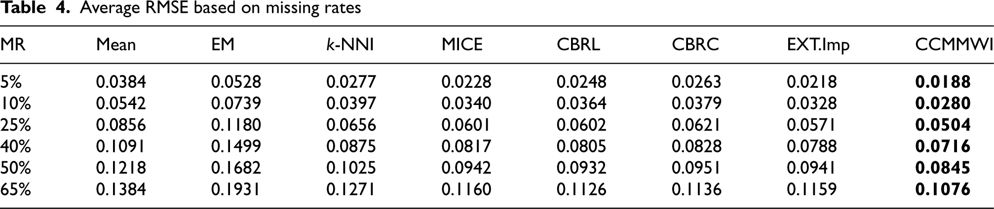
According to the findings in Table 4, the CCMMWI method performs better than the other imputation techniques in terms of RMSE across a variety of missing rates, including minor, moderate, high, and extremely high missing rates. In this instance, the CCMMWI consistently yields lower RMSE values than the other imputation methods, indicating that it might be more accurate at imputing missing values and generating statistical estimates. The results indicate that achieving a low error rate corresponds to estimating values that closely align with the original data. Despite MICE, CBRL, and CBRC utilizing the same estimator model, Bayesian ridge, variations in error rates arise due to the contribution of features, which has been adjusted based on their correlation with the label feature.
Based on MAE results
This section displays the results of applying various imputation techniques to datasets with varying levels of missing data, as measured by the MAE. The MAE measures the difference between a dataset’s predicted and observed values. It is commonly employed to evaluate the performance of statistical models, including those used for imputing missing data.
Average MAE based on datasets
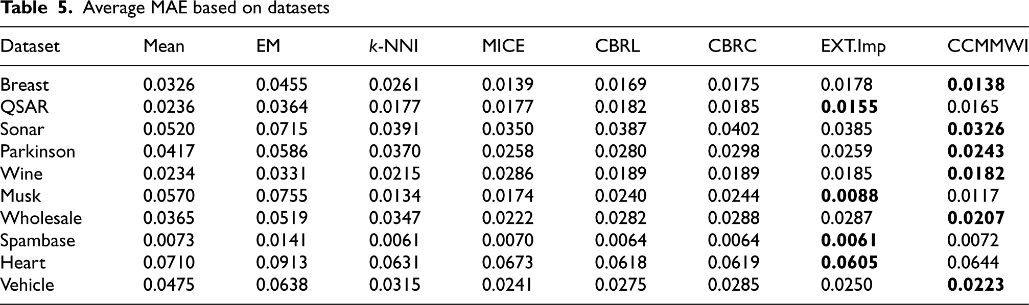
Average MAE based on datasets
According to Table 5, the CCMMWI consistently performs better than the other approaches in terms of MAE across various datasets. In this case, the CCMMWI consistently yields lower MAE values than the other imputation methods in six of ten datasets, indicating that it may be more accurate at imputing missing values and creating statistical estimates. Table 5 also shows that the EXT.Imp method outperforms the other methods in the QSAR, MUSK, Spambase, and Heart datasets. However, k-NNI provides the lower MAE in Spambase dataset sharing with ExtraImpute. In line with the RMSE results, the EM method consistently produces higher MAE values than the other methods in all datasets.
Average MAE based on missing rates

Average MAE based on missing rates
The results in Table 6 show the average MAE values for each imputation technique across the different missing rates in each dataset. Table 6 indicates that CCMMWI outperforms all other techniques under all missing-rate cases. Only with a 5% missing rate that EXT.Imp shows the lower MAE value sharing with CCMMWI.
Based on
results
R-squared (
Average
based on datasets
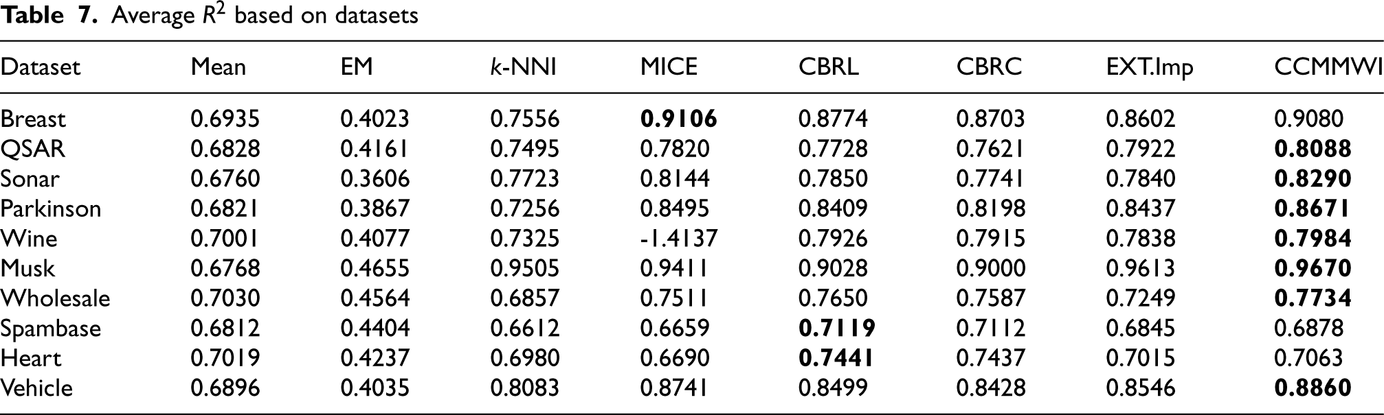
Average
According to Table 7, three of the evaluated methods obtained higher
Average
based on missing rates

Average
Table 8 presents the results of various imputation techniques applied to different datasets with different rates of missing data. The results show that the CCMMWI imputation method consistently produces the highest
Conclusions
In this study, addressing missing data emerges as a crucial aspect of real-world data analysis, with the primary objective being the preservation of all observed data for subsequent analysis. Employing effective strategies for estimating missing data is paramount in overcoming this challenge. The authors conducted a thorough examination of various previously published approaches aimed at handling missing data, evaluating their efficacy across diverse datasets characterized by varying levels of missing values. The study introduces CCMMWI, a novel algorithm utilizing normalized weighted values based on correlation coefficient values to impute missing data. This innovative weighting strategy seeks to optimize the contribution of features by considering their relationships with the target feature. The study’s findings underscore the superior performance of CCMMWI over alternative methods, including Mean, EM, k-NNI, MICE, CBRL, CBRC, and ExtraImpute, as evidenced by accuracy measures and error metrics such as RMSE and MAE. Notably, CCMMWI achieves higher
Footnotes
Acknowledgments
We are very grateful to Universiti Kebangsaan Malaysia for supporting this research, especially to the Data Mining and Optimization (DMO) Research Lab of Fakulti Teknologi dan Sains Maklumat (FTSM), Universiti Kebangsaan Malaysia. Massive appreciation to Universiti Kebangsaan Malaysia for providing grant code GGP-2020-032 for this research funding.