Multi-scale hierarchical model for long-term time series forecasting

Abstract

Long-term time series forecasting (LTSF) has become an urgent requirement in many applications, such as wind power supply planning. This is a highly challenging task because it requires considering both the complex frequency-domain and time-domain information in long-term time series simultaneously. However, existing work only considers potential patterns in a single domain (e.g., time or frequency domain), whereas a large amount of time-frequency domain information exists in real-world LTSFs. In this paper, we propose a multi-scale hierarchical network (MHNet) based on time-frequency decomposition to solve the above problem. MHNet first introduces a multi-scale hierarchical representation, extracting and learning features of time series in the time domain, and gradually builds up a global understanding and representation of the time series at different time scales, enabling the model to process time series over lengthy periods of time with lower computational complexity. Then, the robustness to noise is enhanced by employing a transformer that leverages frequency-enhanced decomposition to model global dependencies and integrates attention mechanisms in the frequency domain. Meanwhile, forecasting accuracy is further improved by designing a periodic trend decomposition module for multiple decompositions to reduce input-output fluctuations. Experiments on five real benchmark datasets show that the forecasting accuracy and computational efficiency of MHNet outperform state-of-the-art methods.

Keywords

Long-term series forecasting multi-scale modeling time-frequency representation time series decomposition

1. Introduction

Time series forecasting has been widely used in various fields such as electricity, energy, climate, and transportation [11,34,7]. Long-term time series forecasting (LTSF), in particular, is challenging due to the uncertainty of forecasting increasing as the forecast horizon extends [32,25,47]. It is crucial for many different types of applications, e.g., transportation participants’ long-term trajectory estimates, long-term renewable energy policies, planning for electricity consumption, environmental monitoring [29,27], etc. Factors like trend changes, structural changes, and external disturbances in long-term time series further complicate forecasting [5].

Making an accurate LTSF model is a difficult undertaking, as both time-domain information (i.e., the sensor data over time) and frequency-domain information (i.e., the information about each frequency component of the sensor data) need to be considered jointly. The equivalent transformation of the two is realized by the Fourier transform. To address this issue, conventional techniques, e.g., Seasonal Auto-Regressive Integrated Moving Average (SARIMA) [37], Gaussian Process (GP) [18], Bayesian Temporal Matrix Factorization (BTMF) [3], and Vector Autoregression Moving-Average with Exogenous Regressors (VARMAX) [12], often cling to the rigid stationary assumption and are unable to account for the non-linear relationships between variables. Over the past few years, deep learning-based methods like recurrent neural networks (RNNs) [21,19], long short-term memory networks (LSTMs) [16,35,48], and transformer-based methods [32,47,41,20,8,46] have made significant innovations in time series forecasting. However, transformer-based methods, due to their computational complexity and memory requirements, struggle with modeling long sequences. Recently, a linear model called DLinear [44] has shown competitive performance in transformer-based methods. However, PatchTST [32], a new transformer-based model to shorten sequence length by patch, achieves awesome results in long-term time series forecasting. Despite the success of various LTSF models, the existing work overlooks two crucial aspects.

Firstly, existing time-domain work [26,24,33] only takes into account time correlations at one time scale, which might not adequately capture the variations found in a wide range of real-world situations. In fact, long-term sequences often exhibit multiple time patterns at different time resolutions (e.g., seconds, minutes, hours), and different time scales are typically associated with different periodic patterns present in the data. For instance, in electricity load forecasting, different hours within a day exhibit different periodicities, and the load also varies from week to week, as shown in Fig. 1. Rich information is provided by these multiscale time patterns for LTSF modeling. Therefore, efficiently capturing long-term dependencies and decomposing multiscale time patterns in time series data is an important challenge for LTSF models.

Figure 1.

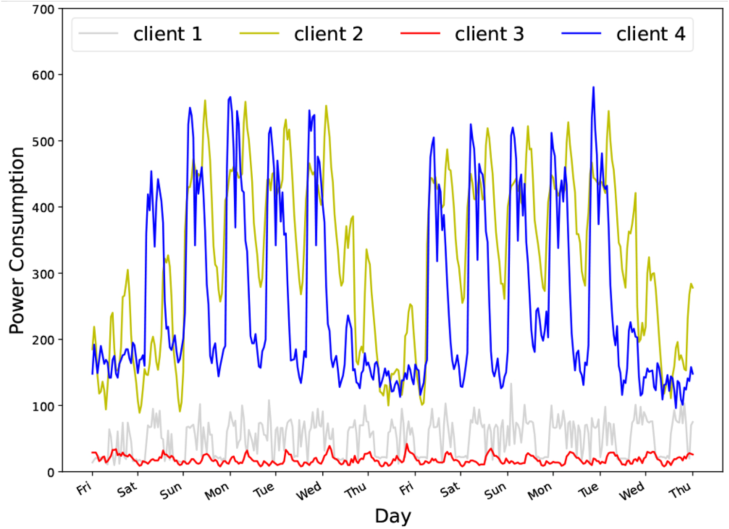
The pattern of power consumption was repeated daily and weekly for client 1 and 3 and weekly for client 2 and 4 in the Electricity dataset during the two-week period from 2:00 on Friday to 23:00 on Thursday.

Secondly, the time-frequency information of long-term time series has not been thoroughly researched. Most existing solutions focus on processing information in a single domain, such as the time domain or the frequency domain. For instance, Autoformer [41] and PatchTST [32] only consider time periodicity and perform semantic learning with an enhanced Transformer structure, while FiLM [46] and FEDformer [47] only focus on the frequency domain. In order to analyze and forecast time series, both time and frequency information are necessary. Time-related periodicity and correlations are captured in the time domain, while global features and potential time series changes are captured in the frequency domain. Thus, integrating time and frequency information in long-term time series to discover interactions between time patterns and frequency components at different time scales is another problem that needs to be urgently addressed in this paper.

In order to address the abovementioned challenges, this paper introduces a multi-scale hierarchical network (MHNet) based on time-frequency decomposition, dedicated to LTSF. MHNet consists of the frequency-enhanced information representation module and the multi-scale time-domain feature extraction module. In the multi-scale time-domain feature extraction module, we adopt a multi-scale hierarchical representation [9] of long-term time series in the time domain. We use window slicing to decompose the data into sub-sequences at multiple scales, extract features, and represent each sub-sequence. This not only allows for the gradual establishment of a global understanding and representation of the time series with different time scales but also enables handling long-term time series data with lower computational complexity and memory overhead. In the frequency-enhanced information representation module, we introduce a transformer based on frequency-enhanced decomposition [47]. It has two advantages: first, it employs a hybrid expert module for seasonal trend decomposition to extract features in the frequency domain, better capturing the global features of the time series. Multiple decompositions can also reduce input-output fluctuations, further improving forecasting accuracy. Second, it is also possible to lower the computational complexity of the transformer by choosing a fixed number of Fourier components at random. By integrating these two ideas, we design a multi-scale window mechanism in MHNet to capture time patterns at different time resolutions, achieving joint modeling of time and frequency domains in long-term time series. The main contributions of this paper are as follows:

Through joint processing of long-term time series in the time and frequency domains, we propose a multi-scale hierarchical network (MHNet) based on time-frequency decomposition for robust and efficient LTSF.

To improve the efficiency of transformers on long sequences, we introduce multi-scale hierarchical representation and Fourier component random selection mechanisms, significantly reducing the computational complexity and memory requirements of the model.

We use five actual benchmark datasets in our extensive experimentation. According to the experimental findings, MHNet performs better in terms of computational efficiency and forecasting accuracy than other methods.

The rest of this paper is arranged as follows:. In the second section, we introduce related work, and in the third section, we provide a detailed explanation of the proposed MHNet framework. In the fourth section, we present the experimental design and settings of the proposed framework. The fifth section concludes the paper.

2. Related work

Long-term time series forecasting (LTSF) [17] refers to the forecasting and analysis of data over an extended future time range, often involving forecasts spanning multiple quarters, years, or even longer timeframes. Such forecasts require consideration of various factors, including seasonal changes, trends, periodicity, and the possibility of outliers. In the following paragraphs, we first present the recent developments in the field of time series forecasting. Then, we describe existing research on multi-scale hierarchical representation strategies that are based on the information domains (such as time and frequency domains) and LTSF models.

2.1. Long-term time series forecasting

The effectiveness of LTSF depends on the capacity of the model to demonstrate significant predictive ability and accurately represent intricate interactions between input and output. Deep learning methods, a type of machine learning approach utilizing neural network models for advanced pattern recognition and automatic feature extraction, have achieved remarkable success in long-term forecasting in recent years.

Common deep learning models include RNN, CNN, Transformer, and hybrid models [5]. However, traditional RNN models may encounter challenges in capturing long-sequence dependencies due to training-related issues such as gradient vanishing and explosion. But variants of RNNs such as LSTM, BiLSTM [28], and GRU [30] can effectively mitigate the aforementioned issues. Convolution kernels, which are usually employed to learn local patterns, limit CNN models’ capacity to capture global trends and periodicity. According to current research, transformer-based forecasting approaches perform better when predicting long sequences. This superiority is mostly attributed to their self-attention mechanism, which dynamically apprehends remote dependencies and thereby enables them to proficiently navigate intricate patterns and protracted temporal relationships.

In the task of time series prediction, the Transformer model treats the time steps of the input sequence as location information, represents the features of each time step as vectors, and employs an encoder-decoder framework for forecasting. Reformer [15] enhances efficiency, accuracy, and scalability by introducing separable convolutional and invertible layers. LogTrans [31] proposes an improvement for Transformer-based time series prediction, addressing two main weaknesses: position-independent attention and memory bottlenecks. However, the computational costs of both aforementioned models still remain relatively high, especially when compared to some lightweight models. Informer [45] adopts a generative decoder, self-attention refinement, and ProbSparse self-attention mechanism, reducing computation time by calculating a portion of the attention matrix. However, it still exhibits significant errors in predicting the peaks and valleys of the curves, making it challenging to meet the increasingly high precision requirements for long sequences. Autoformer [41] introduces a time series decomposition module, enhancing the self-attention module with a self-correlation mechanism to explore data patterns more effectively. However, it overly relies on identifying the periodic characteristics of time series data, making it unsuitable for training on datasets with weak periodicity. FEDformer [47], a model designed from a time-frequency perspective. This model incorporates two attention modules that utilize Fourier and wavelet transforms to process time series data. By applying attention operations in the frequency domain, FEDformer enhances the transformer’s capability to capture features of time series data in the frequency domain.

This paper proposes a time series prediction method that leverages a hierarchical multi-scale representation, fully utilizing temporal and frequency information. The model is designed to capture both time and frequency domain features effectively, considering the importance of capturing features from both perspectives.

2.2. Representation in time-frequency domain

Time series analysis and forecasting heavily depend on time-related correlations and periodicity. In recent years, numerous transformer-based solutions have been put forth in an attempt to capture the temporal and long-range dependencies. For example, Informer [45] introduces the ProbSparse self-attention extractive technique based on KL divergence to reduce model complexity. Autoformer [41] changes the Transformer into a deep decomposition structure and designs self-correlation mechanisms to learn subsequence-level time periodicity. FEDformer [47] uses a Fourier-enhanced structure for linear complexity. Pyraformer [20] applies pyramid attention modules with both inter-scale and intra-scale connections, achieving linear complexity. Non-stationary transformers [22] propose the attention of series stationarity and de-stationarity to over-stabilization. TimesNet [40] analyzes temporal changes within 2D spatial regions across multiple periods. LogTrans [31] reduces spatial complexity by capturing local information through the use of LogSparse [15] design and convolutional self-attention layers.

Bais patterns in the frequency domain are also essential for time series forecasting as they can capture global features and underlying variation patterns within the time series [36]. Therefore, various methods have been developed in recent years that leverage frequency-enhanced structures for time series forecasting. For instance, FEDformer [47] uses a Fourier-enhanced structure for frequency domain mapping. ETSformer [39] replaces the self-attention mechanism in Transformers by using exponential smoothing attention and frequency attention. FiLM [46] utilizes Legendre polynomial projection, and [38] uses Fourier projection to approximate historical information, eliminating any external noise. To directly learn features in the frequency domain, STFNets [43] incorporate the short-time Fourier transform into data processing. Fredo [36] learns in the frequency domain based on the periodic AverageTile model. Floss [42] employs periodic offset and spectral density similarity measures to learn representations with consistent periodicity. To efficiently extract time dependencies, JTFT [4] makes use of the sparsity of time series in the frequency domain along with a limited number of learnable frequencies. However, all the above transformer-based solutions have certain limitations, since the majority of models concentrate on creating new mechanisms to simplify the original attention mechanism in an effort to improve forecasting performance, particularly over longer forecasting horizons. Nonetheless, most models only consider time correlations at a single time scale, overlooking the importance of multi-scale time patterns in time series data with complex periodicity.

2.3. Multi-scale hierarchical representation

In this section, we review various multi-scale hierarchical representation strategies in different domains. Unlike the symbols in language data processing with Transformers, language data are generated by humans, which are highly semantic and information-dense, whereas time series data are naturally redundant. In general, Transformers can only learn feature representation of a fixed scale, making it challenging to capture features at different scales in the time series. Therefore, the hierarchical structure of time series data has two advantages: firstly, multi-scale hierarchical processing can utilize information at different time scales to progressively extract and learn features of the time series, building up a global understanding and representation of the time series, and secondly, this hierarchical strategy significantly reduces the computation length in the encoder, saving a considerable amount of computation cost.

Recently, there has been a significant increase in methods that utilize hierarchical strategies for multi-scale feature extraction. Swin Transformer [23] introduces a universal Transformer backbone that constructs hierarchical feature maps. It starts with small-sized patches and progressively merge adjacent patches in deeper Transformer layers to construct hierarchical representation, and achieve linear computational complexity related to the image size. HiFormer [9] proposes a structure based on a CNN Transformer that effectively combines global and local information. It uses a new Transformer-based fusion method to maintain the richness and consistency of feature representation between different scales for the segmentation task of 2D medical images. By generating feature maps at different scales, MA-CNN [2] applies multi-scale convolution to capture information at different scales along the time axis, so as to capture short-term, medium-term, and long-term dependencies in time series. By learning representations for time series using various scales, Formertime [6] addresses the limitation of Transformer models that can only generate fixed-scale sequence input representations, and can extract local features of time series. Additionally, adopting hierarchical strategies can significantly reduce computational costs. Motivated by Formertime, this paper utilizes window slicing to decompose long-term time series data into sub-sequences at multiple scales and extract features and representations for each sub-sequence.

3. The proposed scheme

Figure 2 introduces the overall framework of the MHNet model. The model consists of two main components: one is the Frequency enhanced Information representation module (FI), inspired by FEDformer [47], and the other is the Multi-scale time-domain Feature Extraction module (MFE). The advantage of FI is its strong ability to capture global features of time series in the frequency domain. However, this module can only learn features at a fixed scale, which is not conducive to learning latent information in time series. MFE addresses such a limitation by progressively extracting and learning features of time series in the time domain with hierarchical multi-scale processing, gradually building a global understanding and representation of time series using information at different time scales.

Figure 2.

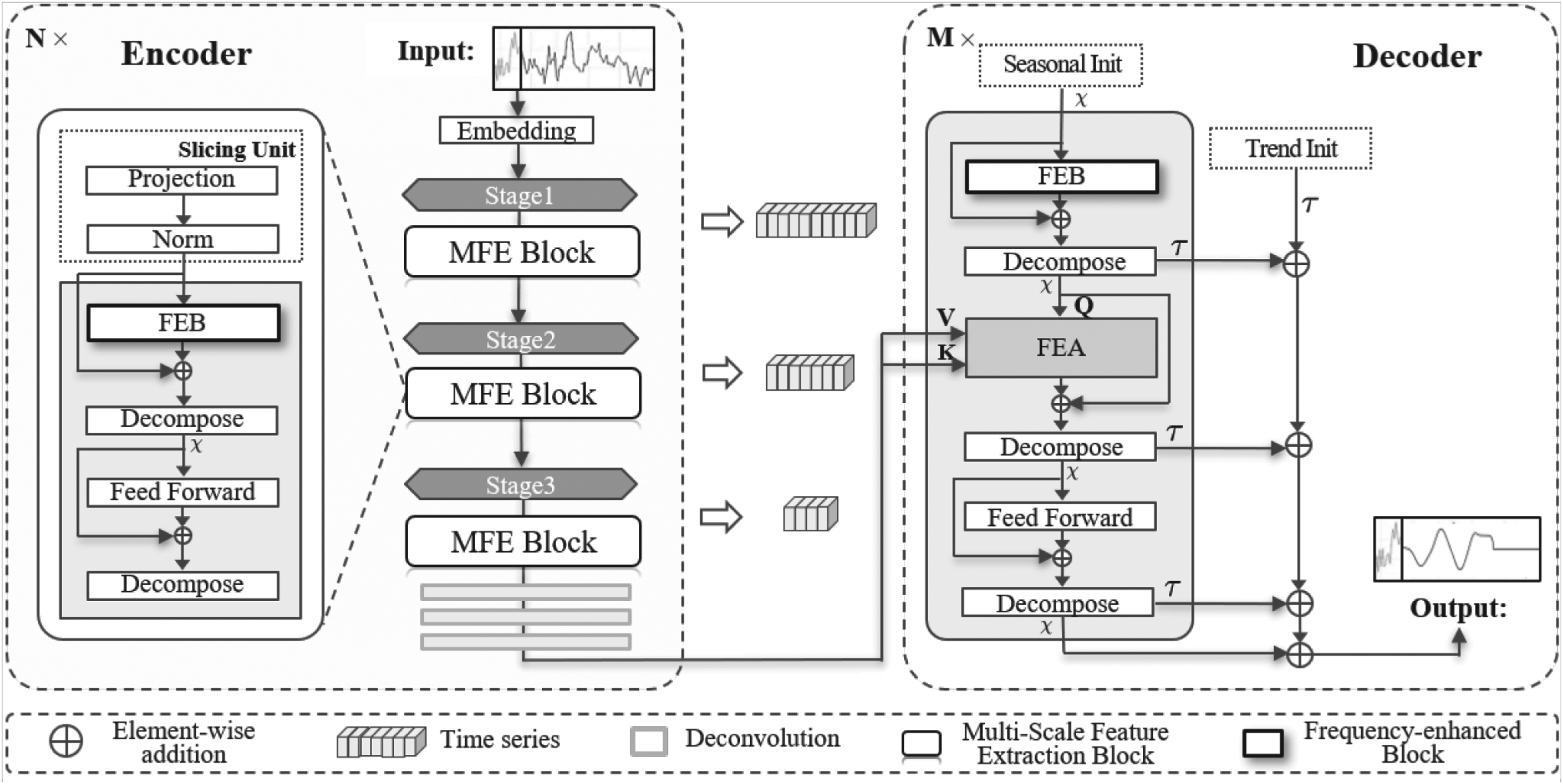
Illustration of the proposed Multi-scale Hierarchical Network (MHNet) based on time-frequency decomposition. MHNet has two primary sections: (a) a multi-scale hierarchical representation, extracting and learning features of time series in the time domain. (b) a Transformer based on frequency-enhanced decomposition to model global dependencies.

3.1. Multi-scale time-domain feature extraction

MFE is illustrated in Fig. 3. A collection of multivariate time series involving numerous channels makes up the model’s whole input. The time series have the same sequence length for every channel. To produce multi-scale representations of time series data, we utilize a hierarchical framework. Specifically, we partition the entire deep neural network architecture into multiple similar stages to generate features across different temporal scales. For the sake of simplicity, each stage’s architecture is analogous, composed of consecutive temporal slice processing operations and our designed time-frequency enhancement decomposition network. In the first stage, our method applies temporal slicing to multivariate time series, with the specific slicing method detailed in Section 3.1.1. Sliced data is then fed into the time-frequency enhancement decomposition module, and the processed data re-enters stage 2 for similar operations, repeating in stage 3 as well. This hierarchical structure enables the effective extraction of time series representations at different scales. Our proposed machine translation model comprises two components: data pre-processing and multi-scale feature extraction module.

Figure 3.

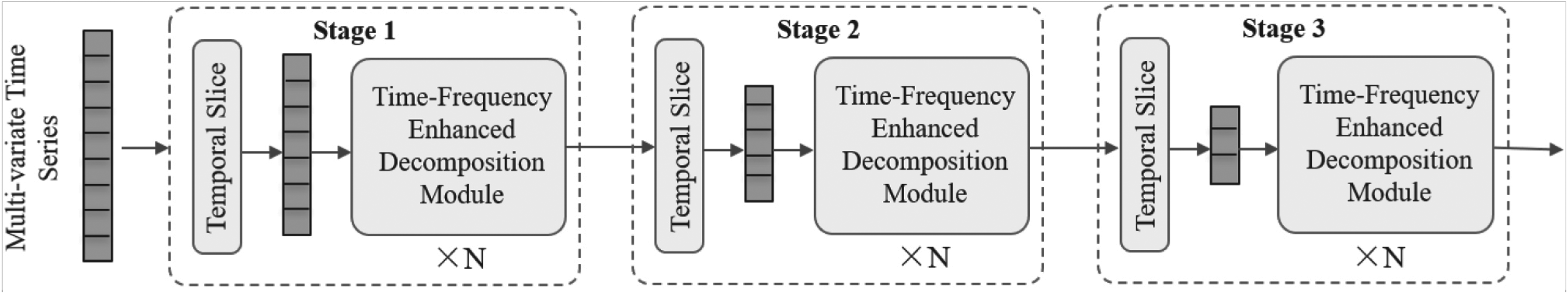
The detailed architecture of the multi-scale time-domain feature extraction module.

3.1.1. Data pre-processing

The data pre-processing phase primarily involves time series slicing, which is the aggregation of consecutive time points, facilitating subsequent operations. Suppose the time series input at stage j, where j is selected from the set 1, 2, 3, is presented as $X = {x_{1}, x_{2}, \dots, x_{l}}$ . Here, l is the length of the input sequence, and $x_{i}$ denotes the data at time point i in the context of the current stage j. If the window slice size is $s_{j}$ , then the aggregation encompasses data from $x_{i}$ to $x_{i} + s_{j}$ for a specific window. In detail, the preprocessing operation utilizes a linear projection layer to project the original sequence into a new channel, transforming the dimensionality of time series from $l * c_{j}$ to $l / s_{j} * C_{j}$ . Here, $c_{j}$ is the number of features in each time point, and $C_{j}$ signifies the new channel created during this stage. The formula is as follows:

\begin{aligned} X^{stage} = Project (X^{stage - 1}) \end{aligned}

(1)

After processing through the projection ction, the input for stage 1 is l*c1, the input for stage 2 is l/s1*C1, the input for stage 3 is l/s1/s2*C2, and the output is l/s1/s2/s3*C3.

This systematic procedure ensures an efficient transformation of the raw time series into a format suitable for subsequent stages, optimizing the representation of temporal information in the computational pipeline.

3.1.2. Multi-scale feature extraction

In the proposed approach, multi-scale feature extraction mainly focuses on the encoder part of the model, which divides the model into three stages. Each stage processes time series data at different scales and uses the output of the previous stage as input to extract features. For example, assuming the input sequence has a size of l in the first stage, we first aggregate $s_{j}$ data points in the time series data into a slice and extract features from this slice data. The output of this stage serves as the input for the next stage. After processing through the three stages, the final output is the extracted features. To maintain consistency with the processing, we apply three times of deconvolution of the features, to map them to the channels required for the decoder. By performing time slicing, different time scales of time series are processed in three stages, progressively extracting and learning time series features.

There are two advantages of introducing hierarchical multi-scale representation in time series forecasting: firstly, hierarchical multi-scale processing can make use of information at different time scales, progressively extract and learn time series features, and gradually build a global understanding and representation of time series. Secondly, through this hierarchical strategy, the length of the entire time series before input to the encoder can be significantly reduced, saving a considerable amount of computational costs.

3.2. Frequency enhanced information representation

This section provides a detailed explanation of a frequency-domain enhancement information representation method based on Transformer, mainly consisting of typical encoder-decoder structure, frequency-domain enhancement mechanism, and time series decomposition mechanism.

3.2.1. Encoder-decoder

Our approach uses a three-stage encoder to learn global feature representations, with each encoder applying the same processing procedure. The encoder adopts a multi-layer structure and can be represented as $X_{e n}^{l} = Encoder (X_{e n}^{l - 1})$ , where $l \in {1, \dots, N}$ represents the number of layers. $X_{e n}^{l}$ represents the output of the l-th encoder layer. The output of each encoder layer serves as the input for the next encoder layer, going through the frequency-domain enhancement module, decomposition module, and feedforward neural network module at one attempt. The specific computation is as follows:

\begin{aligned} S_{e n, -}^{l, 1} & = Decompose (FEB (X_{e n}^{l - 1}) + X_{e n}^{l - 1}) \end{aligned}

(2)

\begin{aligned} S_{e n, -}^{l, 2} & = Decompose (FeedForward (S_{e n}^{l, 1}) + S_{e n}^{l, 1}) \end{aligned}

(3)

\begin{aligned} X_{e n}^{l - 1} & = S_{e n}^{l, 2} \end{aligned}

(4)

In the above equation, $S_{e n}^{l, i}$ , $i \in {1, 2}$ stands for the seasonal components after the i-th time-series decomposition module in the l-th layer. − represents the discarded trend component, indicating that only features of seasonal components are retained in the encoder. The frequency enhancement module (FEB) in Eqs (2)–(4) can be achieved through discrete Fourier transform (DFT) mechanism and is an alternative to the Transformer’s self-attention module.

Additionally, the decoder also uses a multi-layer architecture to processes the seasonal components and trend components of the time series. The structure is represented as $X_{e n}^{l}, T_{d e}^{l} = Decoder (X_{e n}^{l - 1}, T_{d e}^{l - 1})$ , where $X_{e n}^{l}, T_{d e}^{l}$ are the outputs of the l-th layer decoder, $i \in {1, 2, \dots, M}$ . The computation process for the decoder is as follows:

\begin{aligned} S_{d e}^{l, 1}, T_{d e}^{l, 1} & = Decompose (FEB (X_{d e}^{l - 1}) + X_{d e}^{l - 1}) \end{aligned}

(5)

\begin{aligned} S_{d e}^{l, 2}, T_{d e}^{l, 2} & = Decompose (FEA (S_{d e}^{l, 1}, X_{d e}^{N}) + S_{d e}^{l, 1}) \end{aligned}

(6)

\begin{aligned} S_{d e}^{l, 3}, T_{d e}^{l, 3} & = Decompose (FeedForward (S_{d e}^{l, 2}) + S_{d e}^{l, 2}) \end{aligned}

(7)

\begin{aligned} X_{d e}^{l} & = S_{d e}^{l, 3} \end{aligned}

(8)

\begin{aligned} T_{d e}^{l} & = T_{d e}^{l - 1} + W_{l, 1} \cdot T_{d e}^{l, 1} + W_{l, 2} \cdot T_{d e}^{l, 2} + W_{l, 3} \cdot T_{d e}^{l, 3} \end{aligned}

(9)

where the seasonal components and trend components are represented by

S_{d e}^{l, i}

T_{d e}^{l, i}

i \in {1, 2, 3}

in the l-th layer following the i-th decomposition block. The linear weights for the i-th extracted trend

T_{d e}^{l, i}

are represented by

W_{l, i}

i \in {1, 2, 3}

Similar to FEB, FEA is also implemented using a discrete Fourier transform mechanism and can replace the cross-attention module. The final forecasting result is the sum of the two fine decomposition components, i.e., $T_{d e}^{M} + W_{S} \cdot X_{d e}^{M}$ , where $W_{S}$ projects the seasonal component $X_{d e}^{M}$ into the target channel.

3.2.2. Frequency enhanced mechanism

In our plan, the frequency-domain enhancement mechanism consists of two parts, as shown in Fig. 4: the Frequency Enhancement Block (FEB) on the left and the Frequency Enhancement Attention Block (FEA) on the right. They are explained as follows.

Figure 4.

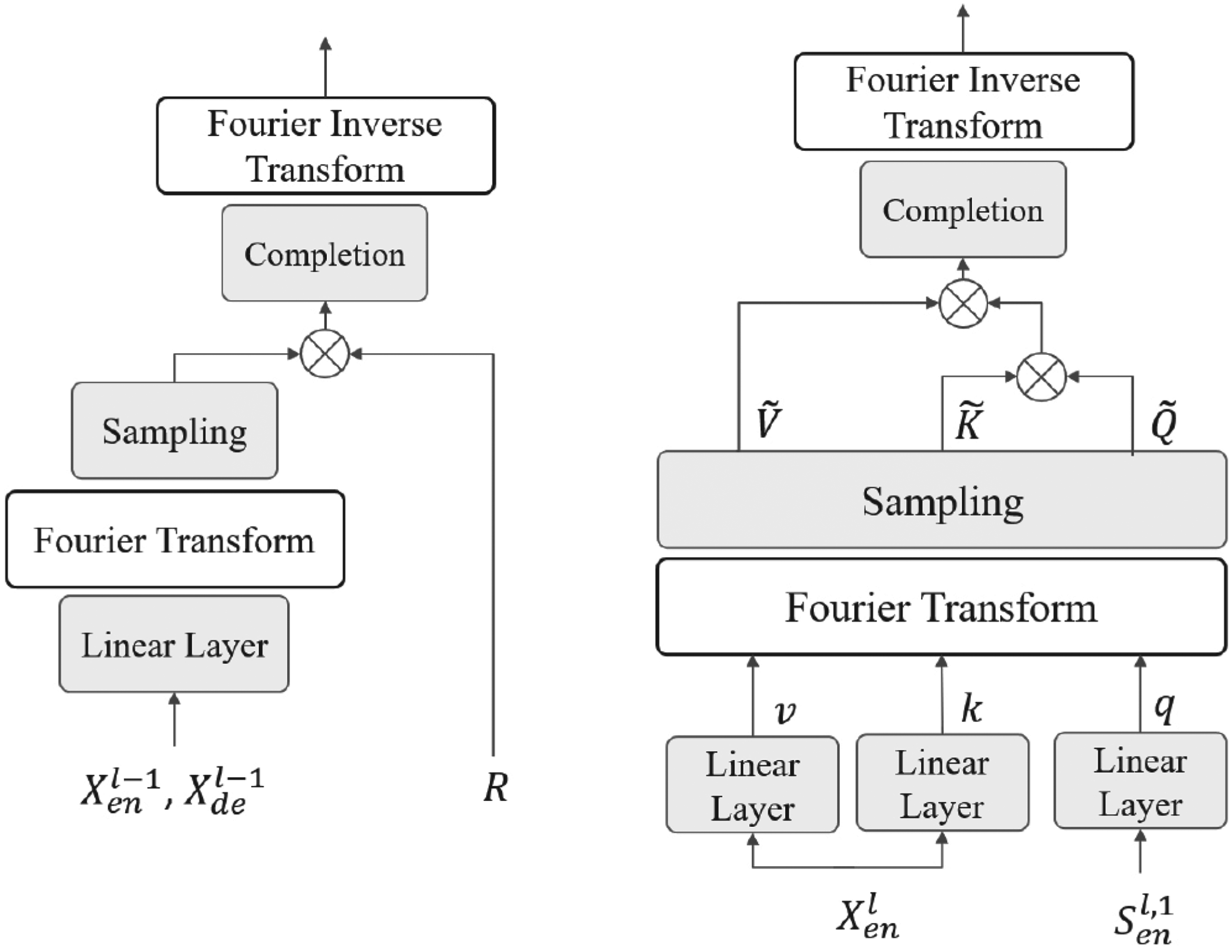
Left: The Frequency Enhancement Block (FEB), Right: The Frequency Enhancement Attention Block (FEA). In FEB, the Fourier transform is used to convert time series into the frequency domain, and the inverse Fourier transform is used to return the sequence to the time domain.

In the Frequency Enhancement Block (FEB), we use the Fourier transform to convert time series into the frequency domain, so as to enhance sequence information. Specifically, a one-dimensional Fourier transform is used to convert the sequence first into the frequency domain. Then, the frequencies are weighted to enhance the relevant information of the sequence. The enhanced sequence is then obtained by applying an inverse Fourier transform to the sequence to return it to the time domain. Replacing the self-attention module with the FEB module can better extract global features of time series. The calculation formula for FEB is as follows:

\begin{aligned} \tilde{Q} & = Select (Q) = Select (F (q)) \end{aligned}

(10)

\begin{aligned} FEB (q) & = F^{- 1} (Padding (\tilde{Q} ⊙ R)) \end{aligned}

(11)

In the above equation, represents the Fourier transform, and represents the inverse Fourier transform. The Fourier transform of q is represented as Q, $Select (\cdot)$ represents the sampling of frequency domain information, retaining M Fourier components ( $M ≪ N$ ). $Padding (\cdot)$ is used to pad the frequency domain information with zeros to fill M dimensions to N dimensions. $R \in C^{D \times D \times M}$ is a randomly initialized parameterized kernel used for frequency weighting.

The Frequency Enhancement Attention Block (FEA) is an attention mechanism that enhances sequence information using Fourier transform. Unlike traditional attention mechanisms, FEA maps the sequence to the frequency domain and calculates attention weights in that domain to enhance sequence information. Replacing the traditional cross-attention block with FEA can further improve sequence modeling capability. Specifically, we process the data in a way similar to FEB. The sequence is first transformed into the frequency domain using one-dimensional Fourier transform. Then, attention weights in the frequency domain are calculated, and then the sequence is transformed back into the time domain to obtain the enhanced sequence. The formula for calculating cross attention in the known Transformer is as follows:

\begin{aligned} Atten (q, k, v) = Softmax (\frac{q k^{⊤}}{\sqrt{d_{q}}}) v \end{aligned}

(12)

In the FEA module, we define the frequency domain enhanced attention module as follows:

\begin{aligned} \tilde{Q} & = Select (F (q)) \end{aligned}

(13)

\begin{aligned} \tilde{K} & = Select (F (k)) \end{aligned}

(14)

\begin{aligned} \tilde{V} & = Select (F (v)) \end{aligned}

(15)

\begin{aligned} FEA (q, k, v) & = F^{- 1} (Padding (σ (\tilde{Q} \cdot {\tilde{K}}^{⊤}) \cdot \tilde{V})) \end{aligned}

(16)

In the above equation, q, k, v represent query, key, and value, and $σ (\cdot)$ represents the activation function. We apply the activation function $σ$ to the output of each neuron. The choice of activation function depends on the dataset, and we typically adopt softmax or tanh, as their convergence performance varies on different datasets.

3.2.3. Time-series decomposition mechanism

Time series decomposition method has been a very useful method in time series analysis. This method assumes that a time series is often a superposition or coupling of various forms of changes: Secular Trend (T), which refers to the overall trend or state that develops and changes over a long period; Seasonal Variation (S), which refers to regular changes in a time series due to seasonal variations; Cyclical Variation (C), which refers to cyclist continuous variations with no strict regularity over several years or cycles; Irregular Variation (I), which is the influence of various accidental factors on the development of time series.

To learn complex time patterns in long-term time series, we introduce the concept of time series decomposition in this paper, where we decompose the input data into seasonal components and trend components, allowing us to process different parts of the data accordingly. When calculating the trend component, we can obtain:

\begin{aligned} X_{trend~} = Softmax (L (x)) * (F (x)) \end{aligned}

(17)

where we use a set of average-pooling filters

F (\cdot)

to extract multiple trend components from the input data, and then use

Softmax (L (x))

as weights to combine these extracted trends.

The above explanation covers the frequency-domain feature extraction based on FEDformer. The following section will provide a detailed explanation of the overall flow of the model.

3.3. Overall structure

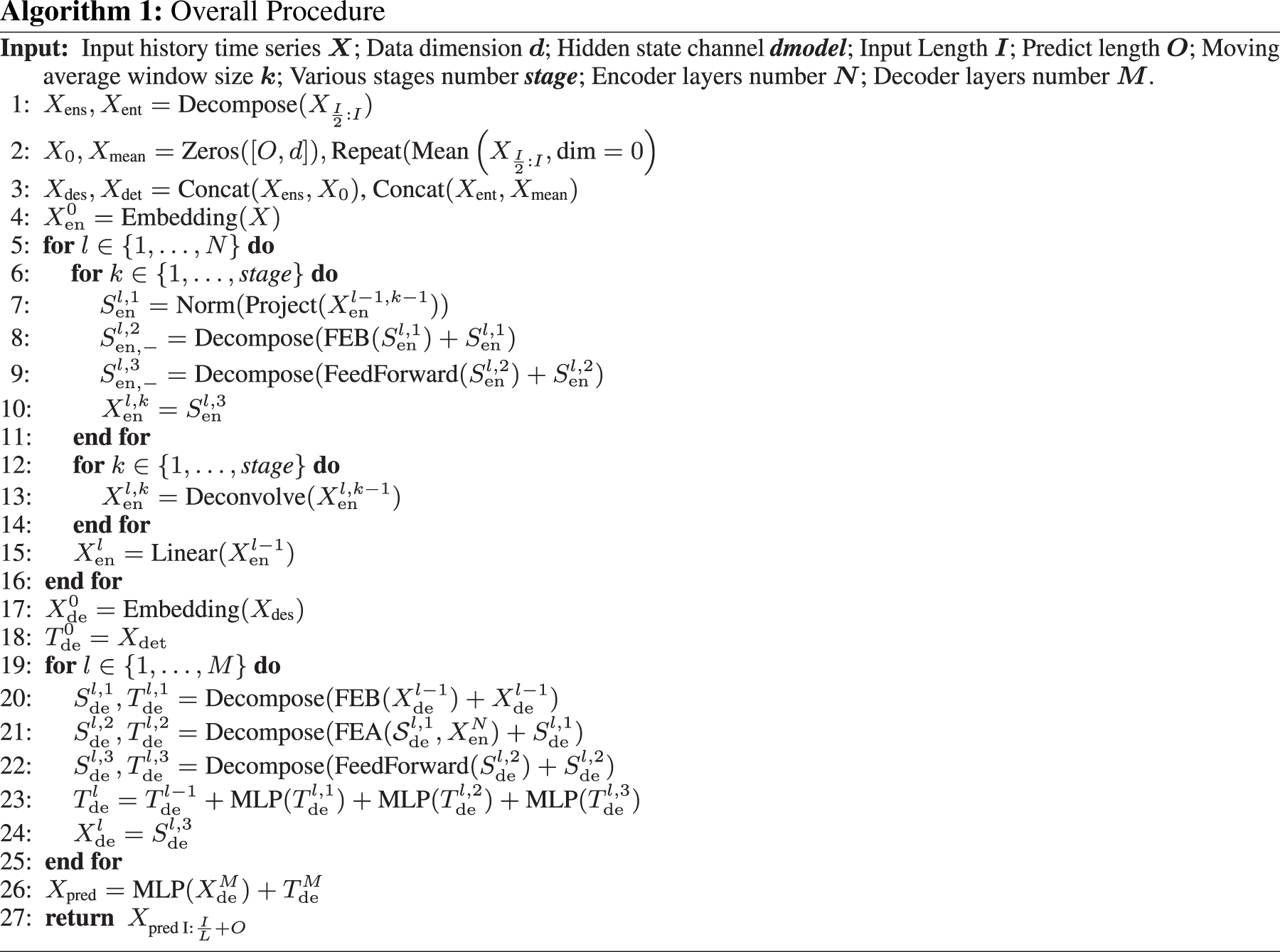
This section provides a detailed explanation of the overall architecture of our proposed MHNet, as shown in Algorithm 1. Assuming historical time series input data $X = {x_{1}, x_{2}, \dots, x_{l}}$ with a length of l, where each time vector $x_{t 1}$ of the t-th time step stands for a multivariate time point with the dimension of D (the multivariate time series’ number of channels), using to forecast time series $\hat{x} = [{\hat{x}}_{l + 1}, \dots, {\hat{x}}_{l + o}]$ , $\hat{x} \in R^{O \times D}$ for future O time steps ( $t > 1$ ).

First, MHNet performs feature extraction in the time domain based on multi-scale hierarchical representation. The consecutive $s_{j}$ data points in the sequence data are aggregated into a slice, and the original features are projected to a new channel $C_{j}$ using a trainable linear projection layer. The sequence data is segmented into three stages, and the fine-grained original time series is processed into a new fine-grained version, which include $l / s_{1}$ s slices, each of the size $s_{1} \times m$ . Then, the linear projection layer projects them into a new channel $C_{1}$ , and the output is constructed as the size $F_{1} \in R^{1 / s_{1} \times C_{1}}$ . Subsequently, the normalized embedding of each time slice and its position embedding are fed into the $l_{1}$ layer. In the same way, the output of the previous stage serves as the input for the next stage, efficiently learning time series representations at different scales by staged spread. Afterward, MHNet performs global feature extraction in the frequency domain based on FEDformer. The encoder first takes the sliced and normalized time sequence data $l \times D$ as input, decomposes the data into seasonal components and trend components through FEB and time series decomposition mechanism. During this process, seasonal components are retained, and trend components are discarded. After three consecutive stages of processing, the seasonal features of original data are obtained, and the data is input into the frequency domain enhancement attention module of the decoder. After three deconvolution operations, the process further continues. In the decoder part, both seasonal and trend components are initialized, and both input sizes are $(l / 2 + O) \times D$ . In the seasonal part, the input is successively processed through FEB and FEA to extract the seasonal features of the time series. After processing each module, all seasonal components and trend components are added together to obtain the final forecasting result.

3.4. Differences compared to FEDformer

As we employ FEDformer as the baseline architecture for the encoder-decoder framework, this section accentuates the divergences between our experiment and FEDformer. In FEDformer, the authors seamlessly integrate a seasonal trend decomposition method into the Transformer-based approach, merging Fourier analysis with Transformer-based methodologies to capture global features of time series in the frequency domain. However, FEDformer exclusively processes time series at a fixed scale, thereby falling short in capturing the local features inherent in time series data.

However, in addressing time series forecasting problems, an excessive emphasis on frequency domain features might result in the oversight of temporal information. In FEDformer, due to the model’s requirement for extracting frequency domain features, time series are trained with the original scale. However, the temporal redundancy of time points in time series poses challenges, and the information at the original scale may not always be conducive to effectively extracting features at various temporal scales. MHNet leverages a multi-scale hierarchical structure to comprehensively capture temporal features in the time domain, enabling us to better utilize information from different temporal scales and establish an effective representation of both global and local features in time series. This characteristic enhances the model’s performance on long sequences, while the hierarchical processing method significantly reduces computational costs. Specifically, the reduction in time series length during input decoding not only improves computational efficiency but also leads to substantial cost savings.

4. Performance evaluation

4.1. Datasets and settings

Dataset:

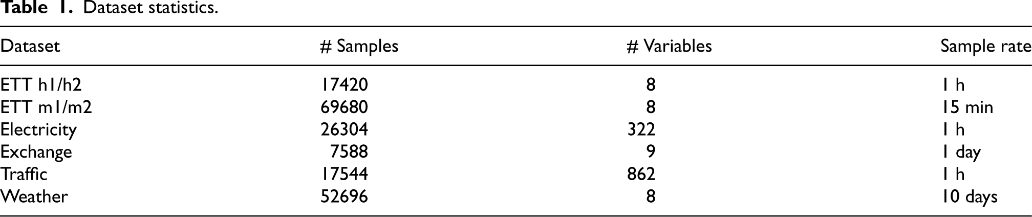
We experiment on five public benchmark datasets (ETT, electricity, exchange-rate, traffic, and weather) to assess MHNet’s performance. The dataset statistics are summarized in Table 1, and the following information is provided regarding the public benchmark datasets that have been fixed:

–
ETT: This dataset is a temperature dataset of electric power Transformers in a county in China collected by Beihang University. It is divided into four types of datasets, namely ETTm1/m2 and ETTh1/h2. Among them, ETTm1/m2 means collecting data once every 15 minutes, and ETTh1/h2 means collecting data once every hour. All datasets include records from July 1, 2016 to June 26, 2018. There are six electric load features and the target value “oil temperature” in each record.
–
Electricity: The dataset involves power consumption data from 321 users, including 26,304 data records from January 1, 2012 to December 31, 2014, with an interval of 1 hour.
–
Exchange-Rate: Exchange-Rate contains eight countries’ daily exchange rates between 1990 and 2016.
–
Traffic: The Traffic dataset records road occupancy rates. It gathers hourly data from 2015 to 2016 that was captured by sensors on San Francisco highways.
–
Weather: This dataset contains local climate data from nearly 1600 regions in the United States. It includes over 35,000 data records from January 1, 2010 to December 31, 2013, with an interval of 1 hour. Each record consists of the target value “wet bulb” and 11 climate features.

The five datasets are divided, in chronological order, into a training set (70%) and a validation set (10%), in accordance with previous works.

Table 1
Dataset statistics.

Dataset # Samples # Variables Sample rate

ETT h1/h2 17420 8 1 h

ETT m1/m2 69680 8 15 min

Electricity 26304 322 1 h

Exchange 7588 9 1 day

Traffic 17544 862 1 h

Weather 52696 8 10 days

Experimental Settings:

MHNet is trained on a single GPU (an NVIDIA GeForce RTX 3080 GPU) and implemented in Python using PyTorch 1.9.0. For experimental settings, the Using the Adam optimizer [13], back-propagation can be used to optimize any parameter that is trainable. The learning rate is set to 1e-3. The number of epochs is set to 10, the dropout rate is 0.05, and the GELU has been chosen as the activation function. To monitor training progress, we implemented an early stopping mechanism, terminating training if there was no evidence of loss degradation on the validation set for three consecutive epochs. To make a fair comparison, all these models are trained under similar settings.

Evaluation Metrics:

Mean Absolute Error (MAE), Mean Square Error (MSE) and R-squared ( $R^{2}$ ) are utilized as metrics for evaluation, which are defined as:
$\begin{aligned} MAE (y, \hat{y}) & = \frac{1}{m} \sum_{i = 1}^{m} (| y_{i} - {\hat{y}}_{i} |) \end{aligned}$
(18)

$\begin{aligned} MSE (y, \hat{y}) & = \frac{1}{m} \sum_{i = 1}^{m} {(y_{i} - {\hat{y}}_{i})}^{2} \end{aligned}$
(19)

$\begin{aligned} R^{2} (y, \hat{y}) & = 1 - \frac{\sum_{i = 1}^{m} {(y_{i} - {\hat{y}}_{i})}^{2}}{\sum_{i = 1}^{m} {(y_{i} - \bar{y})}^{2}} \end{aligned}$
(20)
where MSE can be calculated by first calculating the square of that difference before averaging the findings, in contrast to MAE, which is calculated by determining the absolute value of the difference between each sample’s true value and its predicted value. $R^{2}$ is calculatd as 1 minus the ratio of the sum of the squared differences between the actual and predicted values to the sum of the total squared differences as a measure of the extent to which the model explains the variability in the dependent variable.
4.2. Methods for comparison

Dataset	# Samples	# Variables	Sample rate
ETT h1/h2	17420	8	1 h
ETT m1/m2	69680	8	15 min
Electricity	26304	322	1 h
Exchange	7588	9	1 day
Traffic	17544	862	1 h
Weather	52696	8	10 days

The following are the techniques used in our comparative analysis and the search spaces of their important hyper-parameters:

Deep learning-based Methods:

–
LSTM [10]: It is based on RNN, LSTM establishes internal loops within the unit through input gates, output gates, and forget gates, which solves many problems of RNNs models.
–
LSTNet [14]: It finds long-term patterns of time series trends and extracts short-term local dependency patterns between variables using CNN and RNN. Additionally, it employs traditional Autoregressive (AR) model to address the scale insensitivity issue of neural network models.
–
TCN [1]: It is a CNN-based time convolutional network architecture. It introduces causal convolution and residual connections, which ensure the implementation of CNN in the field of time series prediction with lower memory consumption and parallelism.

Transformer-based Methods:
–
Reformer [15]: It uses LSH (Locality Sensitive Hashing) technology to accelerate the self-attention mechanism, which makes it more efficient and scalable in processing long sequence data
–
LogTrans [31]: It proposes a logarithmic sparse Transformer, which, in the case of a constrained memory budget, raises the time series’ prediction accuracy that have strong long-term dependencies. and fine granularity.
–
Informer [45]: It adopts the generative decoder, self-attention refinement, and ProbSparse self-attention mechanism.
–
Autoformer [41]: It adds a time series decomposition module. It modifies the self-attention module and proposes a self-correlation mechanism that can better explore data patterns.
–
FEDformer [47]: It is a frequency-enhanced decomposed Transformer with a mixed expert mechanism for decomposing periodic and trend components. It replaces the self-attention module and cross-attention module with Fourier-enhanced and Wavelet-enhanced modules. The module can better capture the global features of time series.
–
MHNet: It is our proposed method.

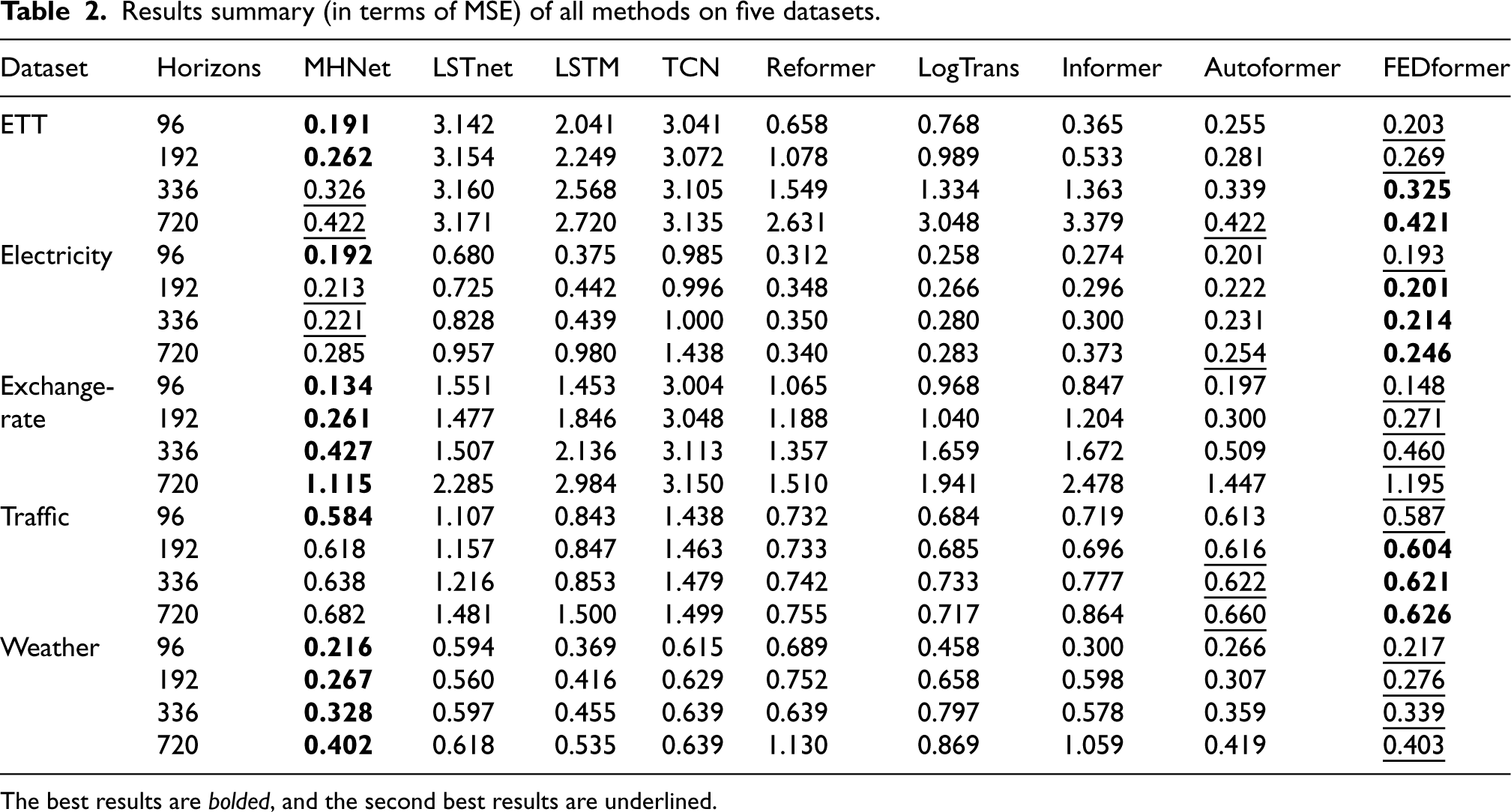
On ETT, Electricity, Exchange-Rate, Traffic and Weather, most baselines (LSTM, LSTNet, TCN, Reformer, Informer, Autoformer, and FEDformer) have been compared in the existing literature. The recurrent layers, convolutional layers, and recurrent-skip layers of LSTM and LSTNet are selected from ${32, 50, 100}$ for their hidden dimension sizes. The output length is selected from ${96, 192, 336, 720}$ , while the input length remains fixed at 96. And we have selected the ETTm2 dataset as the representative for the ETT dataset.
4.3. Main results

The experimental results of all the methods on the five datasets are reported in Tables 2–4, where the following tendencies are apparent.

Table 2
Results summary (in terms of MSE) of all methods on five datasets.

Dataset Horizons MHNet LSTnet LSTM TCN Reformer LogTrans Informer Autoformer FEDformer

ETT 96 0.191 3.142 2.041 3.041 0.658 0.768 0.365 0.255 0.203

192 0.262 3.154 2.249 3.072 1.078 0.989 0.533 0.281 0.269

336 0.326 3.160 2.568 3.105 1.549 1.334 1.363 0.339 0.325

720 0.422 3.171 2.720 3.135 2.631 3.048 3.379 0.422 0.421

Electricity 96 0.192 0.680 0.375 0.985 0.312 0.258 0.274 0.201 0.193

192 0.213 0.725 0.442 0.996 0.348 0.266 0.296 0.222 0.201

336 0.221 0.828 0.439 1.000 0.350 0.280 0.300 0.231 0.214

720 0.285 0.957 0.980 1.438 0.340 0.283 0.373 0.254 0.246

Exchange- 96 0.134 1.551 1.453 3.004 1.065 0.968 0.847 0.197 0.148

rate 192 0.261 1.477 1.846 3.048 1.188 1.040 1.204 0.300 0.271

336 0.427 1.507 2.136 3.113 1.357 1.659 1.672 0.509 0.460

720 1.115 2.285 2.984 3.150 1.510 1.941 2.478 1.447 1.195

Traffic 96 0.584 1.107 0.843 1.438 0.732 0.684 0.719 0.613 0.587

192 0.618 1.157 0.847 1.463 0.733 0.685 0.696 0.616 0.604

336 0.638 1.216 0.853 1.479 0.742 0.733 0.777 0.622 0.621

720 0.682 1.481 1.500 1.499 0.755 0.717 0.864 0.660 0.626

Weather 96 0.216 0.594 0.369 0.615 0.689 0.458 0.300 0.266 0.217

192 0.267 0.560 0.416 0.629 0.752 0.658 0.598 0.307 0.276

336 0.328 0.597 0.455 0.639 0.639 0.797 0.578 0.359 0.339

720 0.402 0.618 0.535 0.639 1.130 0.869 1.059 0.419 0.403

Dataset	Horizons	MHNet	LSTnet	LSTM	TCN	Reformer	LogTrans	Informer	Autoformer	FEDformer
ETT	96	0.191	3.142	2.041	3.041	0.658	0.768	0.365	0.255	0.203
	192	0.262	3.154	2.249	3.072	1.078	0.989	0.533	0.281	0.269
	336	0.326	3.160	2.568	3.105	1.549	1.334	1.363	0.339	0.325
	720	0.422	3.171	2.720	3.135	2.631	3.048	3.379	0.422	0.421
Electricity	96	0.192	0.680	0.375	0.985	0.312	0.258	0.274	0.201	0.193
	192	0.213	0.725	0.442	0.996	0.348	0.266	0.296	0.222	0.201
	336	0.221	0.828	0.439	1.000	0.350	0.280	0.300	0.231	0.214
	720	0.285	0.957	0.980	1.438	0.340	0.283	0.373	0.254	0.246
Exchange-	96	0.134	1.551	1.453	3.004	1.065	0.968	0.847	0.197	0.148
rate	192	0.261	1.477	1.846	3.048	1.188	1.040	1.204	0.300	0.271
	336	0.427	1.507	2.136	3.113	1.357	1.659	1.672	0.509	0.460
	720	1.115	2.285	2.984	3.150	1.510	1.941	2.478	1.447	1.195
Traffic	96	0.584	1.107	0.843	1.438	0.732	0.684	0.719	0.613	0.587
	192	0.618	1.157	0.847	1.463	0.733	0.685	0.696	0.616	0.604
	336	0.638	1.216	0.853	1.479	0.742	0.733	0.777	0.622	0.621
	720	0.682	1.481	1.500	1.499	0.755	0.717	0.864	0.660	0.626
Weather	96	0.216	0.594	0.369	0.615	0.689	0.458	0.300	0.266	0.217
	192	0.267	0.560	0.416	0.629	0.752	0.658	0.598	0.307	0.276
	336	0.328	0.597	0.455	0.639	0.639	0.797	0.578	0.359	0.339
	720	0.402	0.618	0.535	0.639	1.130	0.869	1.059	0.419	0.403

The best results are bolded, and the second best results are underlined.

Table 3

Results summary (in terms of MAE) of all methods on five datasets.

Dataset	Horizons	MHNet	LSTnet	LSTM	TCN	Reformer	LogTrans	Informer	Autoformer	FEDformer
ETT	96	0.283	1.365	1.073	1.330	0.619	0.642	0.453	0.339	0.287
	192	0.326	1.369	1.112	1.339	0.827	0.757	0.563	0.340	0.328
	336	0.364	1.369	1.238	1.348	0.972	0.872	0.887	0.372	0.366
	720	0.421	1.368	1.287	1.354	1.242	1.328	1.388	0.419	0.415
Electricity	96	0.307	0.645	0.437	0.813	0.402	0.357	0.368	0.317	0.308
	192	0.326	0.676	0.473	0.821	0.433	0.368	0.386	0.334	0.315
	336	0.335	0.727	0.473	0.824	0.433	0.380	0.394	0.338	0.329
	720	0.384	0.811	0.814	0.784	0.420	0.376	0.439	0.361	0.355
Exchange-	96	0.261	1.058	1.049	1.432	0.829	0.812	0.752	0.323	0.278
rate	192	0.370	1.028	1.179	1.444	0.906	0.851	0.895	0.369	0.380
	336	0.480	1.031	1.231	1.459	0.976	1.081	1.036	0.524	0.500
	720	0.818	1.243	1.427	1.458	1.016	1.127	1.310	0.941	0.841
Traffic	96	0.367	0.685	0.453	0.784	0.423	0.384	0.391	0.388	0.366
	192	0.387	0.706	0.453	0.794	0.420	0.390	0.379	0.382	0.373
	336	0.400	0.730	0.455	0.799	0.420	0.408	0.420	0.337	0.383
	720	0.428	0.805	0.805	0.804	0.423	0.396	0.472	0.408	0.382
Weather	96	0.284	0.587	0.406	0.589	0.596	0.490	0.384	0.336	0.296
	192	0.324	0.565	0.435	0.600	0.638	0.589	0.544	0.367	0.336
	336	0.367	0.587	0.454	0.608	0.596	0.652	0.523	0.395	0.380
	720	0.420	0.599	0.520	0.610	0.792	0.675	0.741	0.428	0.428

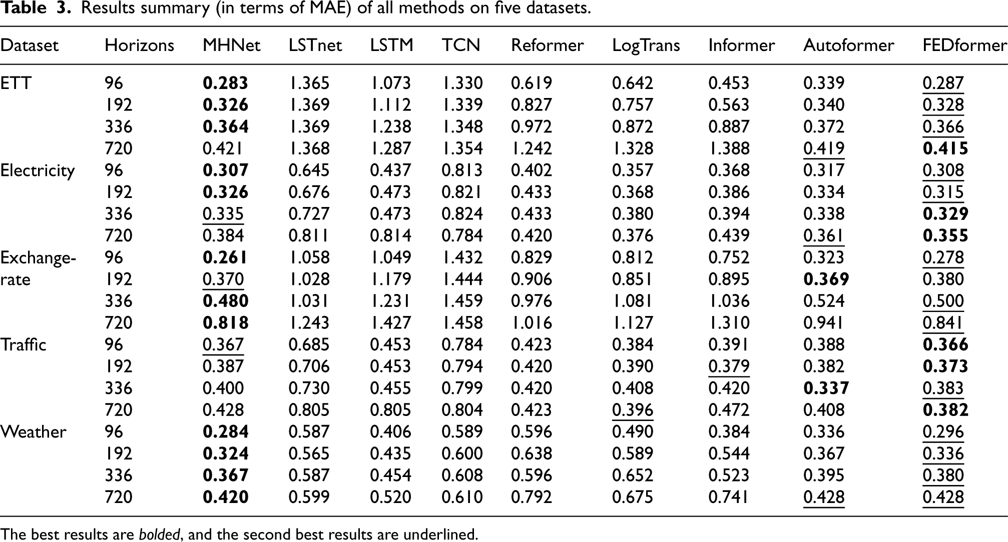
The best results are bolded, and the second best results are underlined.

Table 4

Results summary (in terms of R-squared) of all methods on five datasets.

Dataset	Horizons	MHNet	LSTnet	LSTM	TCN	Reformer	LogTrans	Informer	Autoformer	FEDformer
ETT	96	0.875	0.520	−1.181	−4.980	0.564	0.591	0.774	0.856	0.877
	192	0.831	0.505	−1.268	−5.424	0.421	0.464	0.566	0.821	0.833
	336	0.790	0.494	−1.403	−6.306	0.086	0.449	−1.338	0.785	0.788
	720	0.728	0.481	−0.938	−7.907	−0.964	0.320	−0.868	0.728	0.727
Electricity	96	0.790	0.773	−1.436	−1.309	0.682	0.601	0.522	0.787	0.789
	192	0.789	0.743	−2.169	−1.044	0.681	0.038	0.260	0.751	0.787
	336	0.748	0.685	−3.011	−0.935	0.654	0.026	0.113	0.732	0.769
	720	0.724	0.638	−4.301	−1.027	0.673	0.015	0.086	0.714	0.724
Exchange-	96	0.904	0.559	−1.936	−9.882	0.505	0.499	0.536	0.905	0.908
rate	192	0.837	0.522	−1.739	−10.347	0.157	0.331	0.397	0.837	0.836
	336	0.732	0.259	−3.428	−17.514	−0.237	0.218	0.151	0.663	0.726
	720	0.302	−0.655	−5.134	−18.783	−0.190	−0.197	−0.574	0.292	0.303
Traffic	96	0.592	0.465	−6.645	0.572	0.517	0.493	0.402	0.531	0.536
	192	0.581	0.519	−6.314	0.406	0.521	0.438	0.063	0.561	0.586
	336	0.572	0.474	−11.608	0.311	0.523	0.356	0.033	0.529	0.579
	720	0.551	0.463	−23.932	0.271	0.522	0.359	0.013	0.506	0.577
Weather	96	0.611	0.512	−4.923	0.218	0.159	0.171	−0.100	0.517	0.616
	192	0.465	0.409	−5.367	0.091	0.089	0.054	−0.239	0.474	0.532
	336	0.426	0.379	−6.051	−0.377	0.025	−0.043	−0.325	0.383	0.449
	720	0.283	0.247	−7.217	−1.574	−0.433	−0.186	−1.762	0.272	0.300

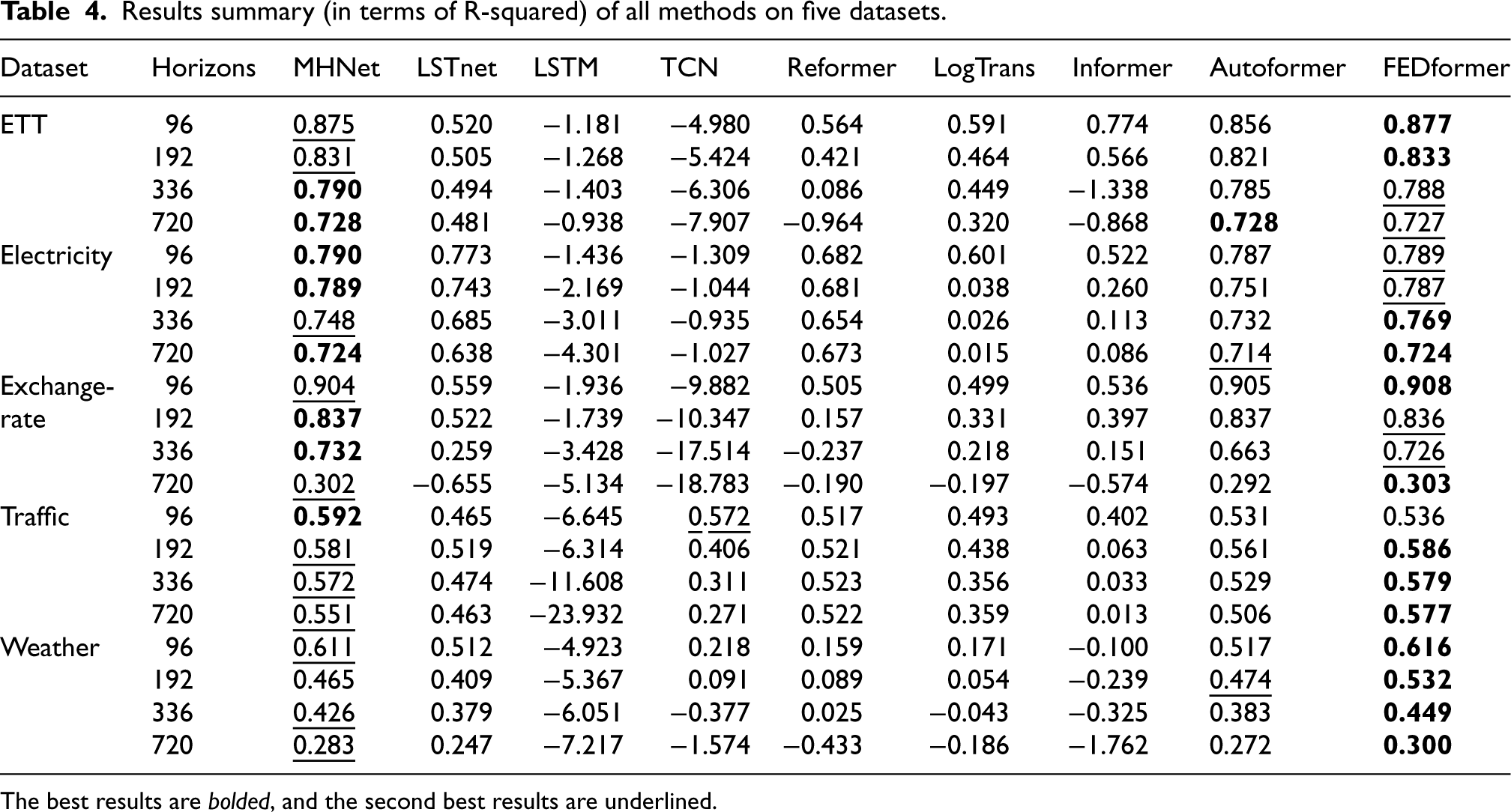
The best results are bolded, and the second best results are underlined.

Our method (MHNet) produces the state-of-the art results. Specifically, MHNet outperforms the current methods on all horizons and all metrics on the Exchange-Rate and Weather datasets. The Exchange-Rate and Weather data, which demonstrate an overall upward or downward trend change with multi-scale structural changes, may be the reason why they are so well suited for our assumption. One possible explanation for this could be the seasonal trend decomposition module. On the Traffic dataset, however, MHNet performs marginally worse than other approaches. The autocorrelation graphs of sample variables from the Exchange-Rate and Traffic datasets are displayed in Fig. 6 to help investigate the causes. We can plainly see the trend and structural changes in the Exchange-Rate dataset. In contrast, for Traffic dataset, we can hardly see the trend changes. In addition, as demonstrated in Table 4, our model exhibits strong performance in terms of the $R^{2}$ metric, consistently outperforming or equaling the results achieved by the baseline models. These findings offer empirical direction for MHNet’s successful modeling of LTSF.

Deep learning-based methods (LSTM, LSTNet, TCN) get worse results then Transformer-based methods, as they cannot capture long-term temporal dependencies. Specifically, when it comes to long-range feature capture ability, the RNN-based LSTM and LSTNet outperforms the CNN-based TCN model by a huge margin. This is due to CNN’s convolutional kernel and receptive filed, which limits its capacity to extract long-range features. Based on the frequency feature extraction ability, the Transformer models outperform the RNN- and CNN-based models by a significant margin.

Transformer-based methods (Reformer, LogTrans, Informer, Autoformer, FEDformer) are the state-of-the-art methods that extend attention modules to learn long-term temporal dependencies. Among them, FEDformer outperforms Informer in all the cases (5 datasets $\times$ 4 horizons) in terms of both MAE and MRE, and exceeds Autoformer in 18 out of 20 cases in terms of MAE metric.

4.4. Effect of multi-scale modeling

Figure 5.

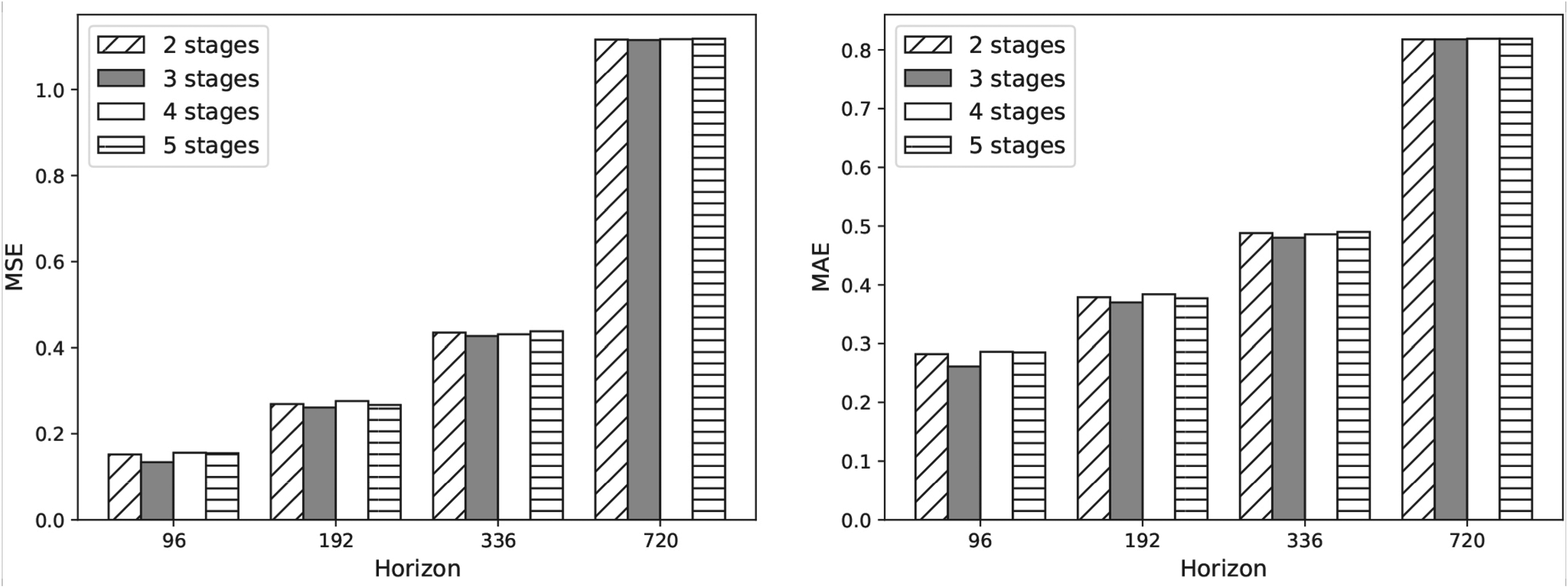
Visualization of results under ${2, 3, 4, 5}$ scales. The left graph represents the evaluation results based on MSE. The right graph depicts the evaluation results based on MAE.

In order to examine the impact of multi-scale modeling, we assess the performance of MHNet across a range of scales (i.e., 2 scales, 3 scales, 4 scales, and 5 scales), and the prediction length ranged from 96 to 720. The Exchange-Rate dataset’s MHNet results under various scale numbers are displayed in Fig. 5. It is evident that MHNet performs better than other scales when the number of scales is increased to three. This is due to MHNet’s increased capacity to identify a wider range of both short- and long-term patterns.

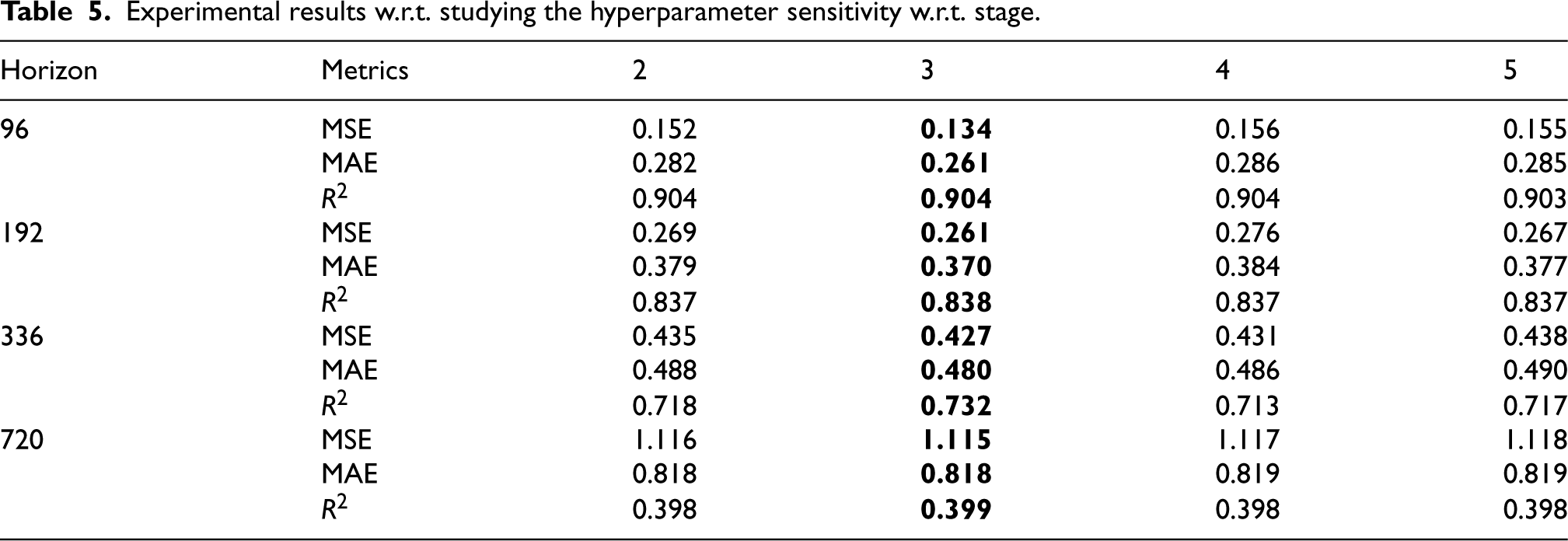
It demonstrates that feature extraction is performed properly using the three-level hierarchical structure. The accuracy of the predictions varies little between the various stages as the prediction length grows. Table 5 displays the specific evaluation values. It is clear that the addition of a hierarchical structure significantly increases the efficiency of the existing time series forecasting model, hence raising the forecasting results’ accuracy. The prediction performance is mediocre when the number of stages is 2, which may be because insufficient parameters will impede the effective information extraction. The performance of MHNet does not improve when the number of stages is increased to 4 or 5, which may be because the task’s requirements for the number of stages have already been satisfied, and over-fitting is easily caused by using too many parameters.

Table 5

Experimental results w.r.t. studying the hyperparameter sensitivity w.r.t. stage.

Horizon	Metrics	2	3	4	5
96	MSE	0.152	0.134	0.156	0.155
	MAE	0.282	0.261	0.286	0.285
	$R^{2}$	0.904	0.904	0.904	0.903
192	MSE	0.269	0.261	0.276	0.267
	MAE	0.379	0.370	0.384	0.377
	$R^{2}$	0.837	0.838	0.837	0.837
336	MSE	0.435	0.427	0.431	0.438
	MAE	0.488	0.480	0.486	0.490
	$R^{2}$	0.718	0.732	0.713	0.717
720	MSE	1.116	1.115	1.117	1.118
	MAE	0.818	0.818	0.819	0.819
	$R^{2}$	0.398	0.399	0.398	0.398

4.5. Parameter study

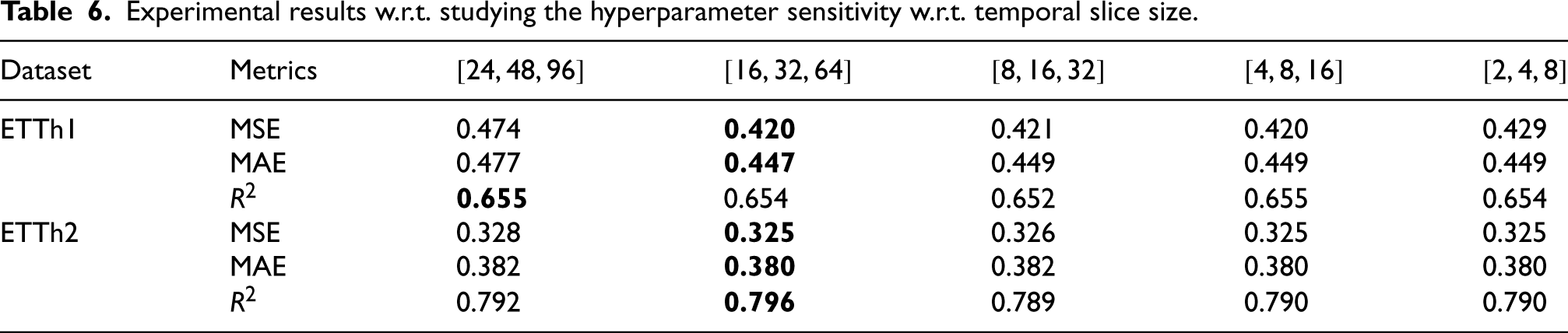
In this section, we examine the two crucial variables (i.e., window slice sizes and learning rate), which could influence the performance of MHNet. Firstly, through a sensitivity study of the hyperparameter window slice size, we validate the value of the multi-scale representation. The window slice sizes for the three stages were set to five different combinations using the ETTh1 and ETTh2 datasets. The predictive performance peaks with the middle three slice sizes, as shown in Table 6, and the highest performance is attained when the slice sizes are $[16, 32, 64]$ . As a result, we decided to use this as the experiment’s default slice option. We hypothesize that latent information cannot be extracted from the time series by using slices that are too big or too small.

Table 6
Experimental results w.r.t. studying the hyperparameter sensitivity w.r.t. temporal slice size.

Dataset Metrics $[24, 48, 96]$ $[16, 32, 64]$ $[8, 16, 32]$ $[4, 8, 16]$ $[2, 4, 8]$

ETTh1 MSE 0.474 0.420 0.421 0.420 0.429

MAE 0.477 0.447 0.449 0.449 0.449

$R^{2}$ 0.655 0.654 0.652 0.655 0.654

ETTh2 MSE 0.328 0.325 0.326 0.325 0.325

MAE 0.382 0.380 0.382 0.380 0.380

$R^{2}$ 0.792 0.796 0.789 0.790 0.790

Dataset	Metrics	$[24, 48, 96]$	$[16, 32, 64]$	$[8, 16, 32]$	$[4, 8, 16]$	$[2, 4, 8]$
ETTh1	MSE	0.474	0.420	0.421	0.420	0.429
	MAE	0.477	0.447	0.449	0.449	0.449
	$R^{2}$	0.655	0.654	0.652	0.655	0.654
ETTh2	MSE	0.328	0.325	0.326	0.325	0.325
	MAE	0.382	0.380	0.382	0.380	0.380
	$R^{2}$	0.792	0.796	0.789	0.790	0.790

Table 7

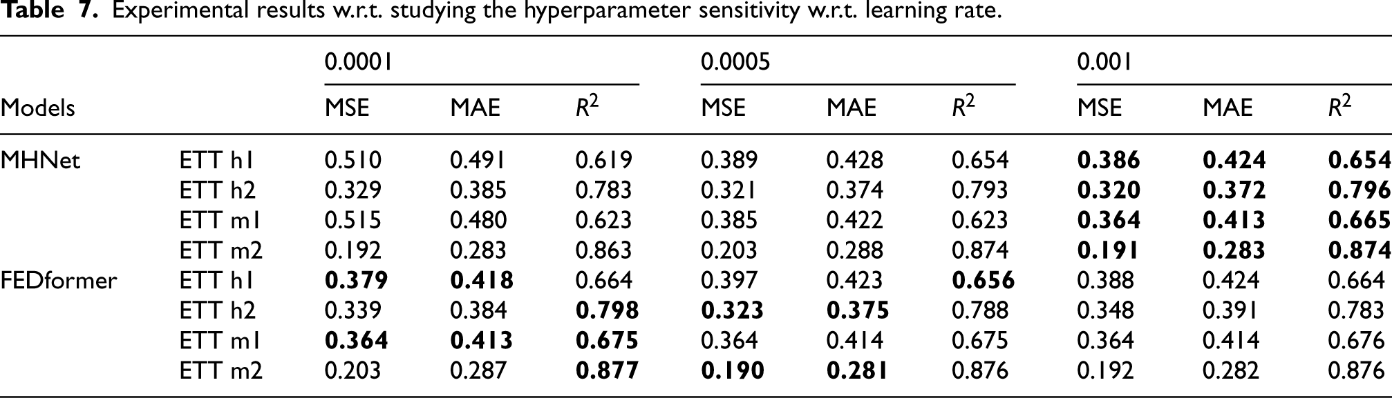
Experimental results w.r.t. studying the hyperparameter sensitivity w.r.t. learning rate.

		0.0001			0.0005			0.001
Models		MSE	MAE	$R^{2}$	MSE	MAE	$R^{2}$	MSE	MAE	$R^{2}$
MHNet	ETT h1	0.510	0.491	0.619	0.389	0.428	0.654	0.386	0.424	0.654
	ETT h2	0.329	0.385	0.783	0.321	0.374	0.793	0.320	0.372	0.796
	ETT m1	0.515	0.480	0.623	0.385	0.422	0.623	0.364	0.413	0.665
	ETT m2	0.192	0.283	0.863	0.203	0.288	0.874	0.191	0.283	0.874
FEDformer	ETT h1	0.379	0.418	0.664	0.397	0.423	0.656	0.388	0.424	0.664
	ETT h2	0.339	0.384	0.798	0.323	0.375	0.788	0.348	0.391	0.783
	ETT m1	0.364	0.413	0.675	0.364	0.414	0.675	0.364	0.414	0.676
	ETT m2	0.203	0.287	0.877	0.190	0.281	0.876	0.192	0.282	0.876

Figure 6.

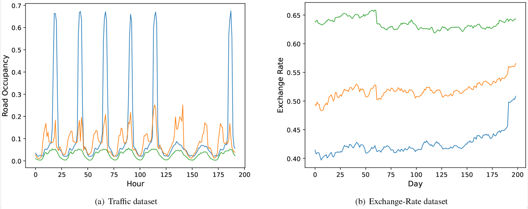
The autocorrelation graphs based on (a) Traffic dataset and (b) Exchange-Rate dataset.

The results of the experiments at various learning rates are then contrasted. We run experiments using the ETTh1 and ETTh2 benchmark datasets in order to assess the performance of MHNet. We discovered that our model operates most effectively when the learning rate is changed to 0.001, as indicated in Table 7, thus we made this choice. When the learning rate is 0.0001, the baseline model operates most effectively. As a result, we decided to use 0.0001 as the baseline model’s learning rate in the experiments.

4.6. Visualization of prediction results

Figure 7 presents a visualization of the prediction results produced by MHNet on five datasets. The ground truth is represented by the blue line, while our predictions are depicted by the orange line. It is observable that the predictive trend of MHNet largely aligns with the original trend analysis. Notably, there are fluctuations in the predictions for the dataset, which we hypothesize may be attributed to the time-frequency transformation mechanism employed in our approach.

4.7. Evaluation of model robustness to noise

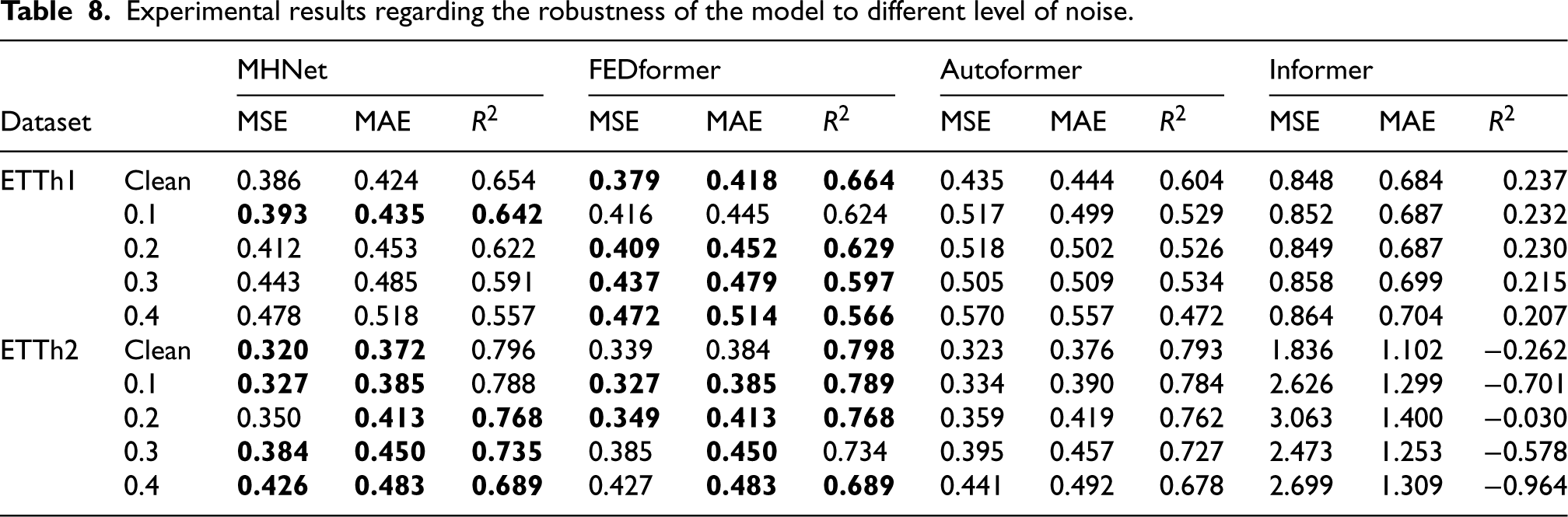
The noise robustness experiment was conducted using the ETTh1 and ETTh2 datasets. We added Gaussian noise to the original datasets, selecting four standard deviations [0.1, 0.2, 0.3, and 0.4] as the noise levels. A larger standard deviation indicates more noise added. The results, as shown in the Table 8, demonstrate that while the performance of our model declines with increasing noise levels, the overall change remains minimal. This indicates that our model is robust to noise. We hypothesize that transforming time series data into the frequency domain can more effectively capture the intrinsic frequency characteristics of the series, thereby enhancing the model’s ability to resist noise. We hypothesize that the model struggles to capture the overall trend of the weather data accurately. Nonetheless, MHNet demonstrated a level of performance that rivals the best models.

Figure 7.

Illustration of the prediction performance using MHNet on five datasets.

Table 8

Experimental results regarding the robustness of the model to different level of noise.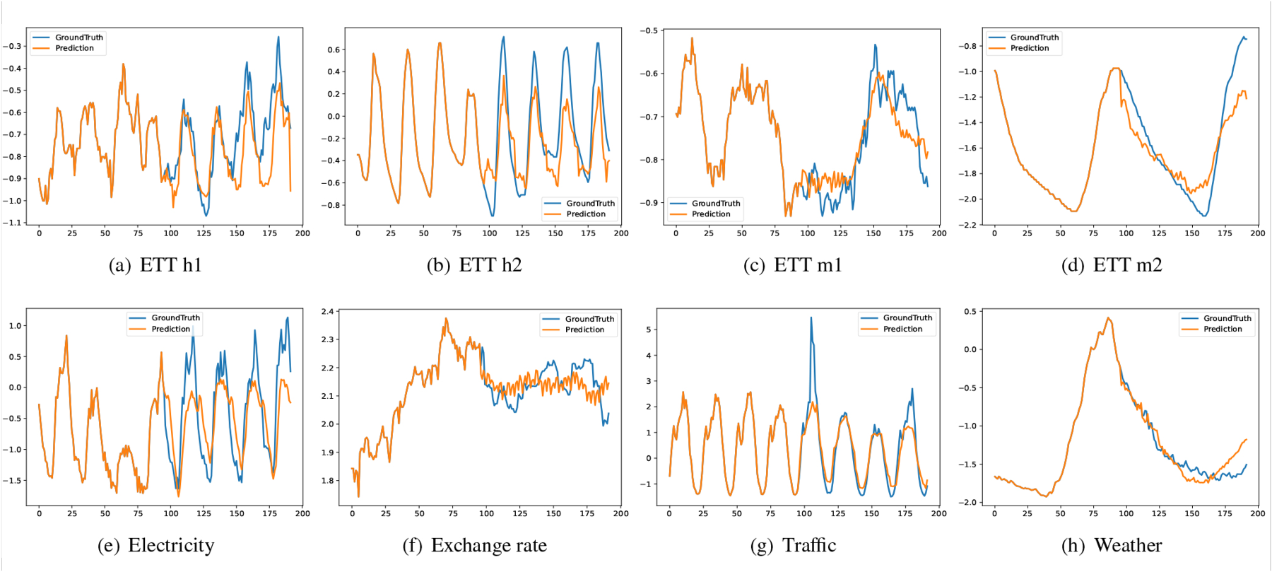

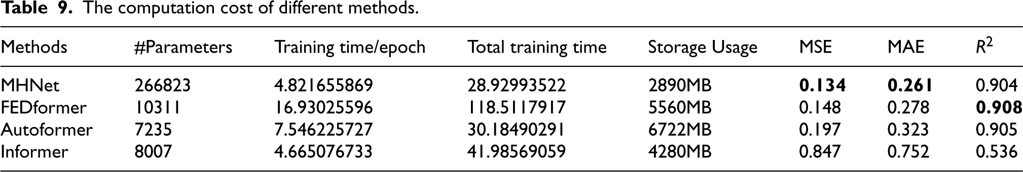
		MHNet			FEDformer			Autoformer			Informer
Dataset		MSE	MAE	$R^{2}$	MSE	MAE	$R^{2}$	MSE	MAE	$R^{2}$	MSE	MAE	$R^{2}$
ETTh1	Clean	0.386	0.424	0.654	0.379	0.418	0.664	0.435	0.444	0.604	0.848	0.684	0.237
	0.1	0.393	0.435	0.642	0.416	0.445	0.624	0.517	0.499	0.529	0.852	0.687	0.232
	0.2	0.412	0.453	0.622	0.409	0.452	0.629	0.518	0.502	0.526	0.849	0.687	0.230
	0.3	0.443	0.485	0.591	0.437	0.479	0.597	0.505	0.509	0.534	0.858	0.699	0.215
	0.4	0.478	0.518	0.557	0.472	0.514	0.566	0.570	0.557	0.472	0.864	0.704	0.207
ETTh2	Clean	0.320	0.372	0.796	0.339	0.384	0.798	0.323	0.376	0.793	1.836	1.102	−0.262
	0.1	0.327	0.385	0.788	0.327	0.385	0.789	0.334	0.390	0.784	2.626	1.299	−0.701
	0.2	0.350	0.413	0.768	0.349	0.413	0.768	0.359	0.419	0.762	3.063	1.400	−0.030
	0.3	0.384	0.450	0.735	0.385	0.450	0.734	0.395	0.457	0.727	2.473	1.253	−0.578
	0.4	0.426	0.483	0.689	0.427	0.483	0.689	0.441	0.492	0.678	2.699	1.309	−0.964

4.8. Computation cost

In models for forecasting time series using Transformers, computational cost has been a significant problem. A high number of parameters are needed for Transformer computing because of the unique characteristics of attention matrix calculation in Transformer models. In order to assess the computational expense, we evaluate the parameter numbers, training time, storage usage and prediction performances of MHNet, FEDformer, Autoformer and Informer on Exchange Rate dataset in Table 9. In these methods, the autoformer has the fewest parameters and operates quickly. However, the forecasting outcomes worsen. Compared with FEDformer and Informer, MHNet runs fastest and gets best forecasting performance improvement and the computation cost. This is because we model the original time series with a hierarchical structure, which greatly reduces the length of the sequence for attentional computation. MHNet demonstrates the superiority over existing methods.

Table 9
The computation cost of different methods.

Methods #Parameters Training time/epoch Total training time Storage Usage MSE MAE $R^{2}$

MHNet 266823 4.821655869 28.92993522 2890MB 0.134 0.261 0.904

FEDformer 10311 16.93025596 118.5117917 5560MB 0.148 0.278 0.908

Autoformer 7235 7.546225727 30.18490291 6722MB 0.197 0.323 0.905

Informer 8007 4.665076733 41.98569059 4280MB 0.847 0.752 0.536

Methods	#Parameters	Training time/epoch	Total training time	Storage Usage	MSE	MAE	$R^{2}$
MHNet	266823	4.821655869	28.92993522	2890MB	0.134	0.261	0.904
FEDformer	10311	16.93025596	118.5117917	5560MB	0.148	0.278	0.908
Autoformer	7235	7.546225727	30.18490291	6722MB	0.197	0.323	0.905
Informer	8007	4.665076733	41.98569059	4280MB	0.847	0.752	0.536

5. Conclusion and future work

In this paper, we propose a multi-scale hierarchical network (MHNet) based on time-frequency decomposition. In order to deal with long time series with lower computational complexity, MHNet first introduces multi-scale hierarchical representations. Then, through a gradual process of extraction and learning of the local dependencies of the time series, it uses the local information of different time scales to gradually build up the global understanding and representations of the time series. This makes it possible for the proposed model to reduce the computational burden of managing long time series. The Transformer then establishes the long-term dependence based on frequency-enhanced decomposition, and the periodic trend term decomposition module is meant to further increase prediction accuracy by reducing input and output fluctuation through numerous decompositions. To strengthen the robustness against noise, attention mechanisms are also used in the frequency domain. Tests conducted on five real-world datasets demonstrate that MHNet performs better in different scenarios than alternative Transformer-based and hybrid approaches. We believe that MHNet can accurately capture the trend changes and structural changes for long-term time series forecasting through theoretical analysis and experimental validation.

Currently, we are still working on extending the hierarchical multi-scale structure. However, adaptively selecting suitable segment sizes for different phases of time series remains a challenge. In our future work, we will further investigate adaptive selection of scales for different stages.

Footnotes

Acknowledgments

This work has been supported by the Jiangsu Provincial Program for Innovation & Entrepreneurship under Grant No.JSSCBS20220406, the Natural Science Research of Jiangsu Higher Education Institutions of China under Grant No.22KJD520004, the General Project of Philosophy and Social Science Research in Jiangsu Colleges and Universities under Grant No.2022SJYB0243.

References

Bai

Kolter

J.Z.

Koltun

, An empirical evaluation of generic convolutional and recurrent networks for sequence modeling, arXiv preprint arXiv:1803.01271, 2018.

Chen

Shi

, Multi-scale attention convolutional neural network for time series classification, Neural Networks 136 (2021), 126–140.

Chen

Sun

, Bayesian temporal factorization for multidimensional time series prediction, IEEE Transactions on Pattern Analysis and Machine Intelligence 44(9) (2021), 4659–4673.

Chen

Liu

Yang

Jing

Zhao

Yang

, A joint time-frequency domain transformer for multivariate time series forecasting, arXiv preprint arXiv:2305.14649, 2023.

Chen

Wang

, Long sequence time-series forecasting with deep learning: A survey, Information Fusion 97 (2023), 101819.

Cheng

Liu

Luo

Chen

, Formertime: Hierarchical multi-scale representations for multivariate time series classification, in: Proceedings of the ACM Web Conference 2023, 2023, pp. 1437–1445.

Di Mauro

Galatro

Postiglione

Song

Liotta

, Multivariate time series characterization and forecasting of voip traffic in real mobile networks, IEEE Transactions on Network and Service Management, 2023.

Wei

, Preformer: predictive transformer with multi-scale segment-wise correlations for long-term time series forecasting, in: ICASSP 2023–2023 IEEE International Conference on Acoustics, Speech and Signal Processing (ICASSP), IEEE, 2023, pp. 1–5.

Heidari

Kazerouni

Soltany

Azad

Aghdam

E.K.

Cohen-Adad

Merhof

, Hiformer: Hierarchical multi-scale representations using transformers for medical image segmentation, in: Proceedings of the IEEE/CVF Winter Conference on Applications of Computer Vision, 2023, pp. 6202–6212.

10.

Hochreiter

Schmidhuber

, Long short-term memory, Neural Computation 9(8) (1997), 1735–1780.

11.

Husnoo

M.A.

Anwar

Hosseinzadeh

Islam

S.N.

Mahmood

A.N.

Doss

, A secure federated learning framework for residential short term load forecasting, IEEE Transactions on Smart Grid, 2023.

12.

Jamdade

P.G.

Jamdade

S.G.

, Modeling and prediction of covid-19 spread in the philippines by october 13, 2020, by using the varmax time series method with preventive measures, Results in Physics 20 (2021), 103694.

13.

Kingma

D.P.

, Adam: A method for stochastic optimization, arXiv preprint arXiv:1412.6980, 2014.

14.

Lai

Chang

W.-C.

Yang

Liu

, Modeling long-and short-term temporal patterns with deep neural networks, in: The 41st International ACM SIGIR Conference on Research & Development in Information Retrieval, 2018, pp. 95–104.

15.

Jin

Xuan

Zhou

Chen

Wang

Y.-X.

Yan

, Enhancing the locality and breaking the memory bottleneck of transformer on time series forecasting, Advances in neural information processing systems, 2019, 32.

16.

Zhu

Kong

Han

Zhao

, Ea-lstm: Evolutionary attention-based lstm for time series prediction, Knowledge-Based Systems 181 (2019), 104785.

17.

Lim

Zohren

, Time-series forecasting with deep learning: A survey, Philosophical Transactions of the Royal Society A, 379(2194) (2021), 20200209.

18.

Lin

Chen

Liu

Lin

Liang

, Gaussian process regression-based forecasting model of dam deformation, Neural Computing and Applications 31 (2019), 8503–8518.

19.

Lin

Zhao

Zhang

, Segrnn: Segment recurrent neural network for long-term time series forecasting, arXiv preprint arXiv:2308.11200, 2023.

20.

Liu

Liao

Lin

Liu

A.X.

Dustdar

, Pyraformer: Low-complexity pyramidal attention for long-range time series modeling and forecasting, in: International Conference on Learning Representations, 2021.

21.

Liu

Gong

Yang

Chen

, Dstp-rnn: A dual-stage two-phase attention-based recurrent neural network for long-term and multivariate time series prediction, Expert Systems with Applications 143 (2020), 113082.

22.

Liu

Wang

Long

, Non-stationary transformers: Exploring the stationarity in time series forecasting, Advances in Neural Information Processing Systems 35 (2022), 9881–9893.

23.

Liu

Lin

Cao

Wei

Zhang

Lin

Guo

, Swin transformer: Hierarchical vision transformer using shifted windows, in: Proceedings of the IEEE/CVF International Conference on Computer Vision, 2021, pp. 10012–10022.

24.

Luo

Chen

Yoshioka

, Dual-path rnn: efficient long sequence modeling for time-domain single-channel speech separation, in: ICASSP 2020-2020 IEEE International Conference on Acoustics, Speech and Signal Processing (ICASSP), IEEE, 2020, pp. 46–50.

25.

Luo

Lyu

Huang

, Tfdnet: Time-frequency enhanced decomposed network for long-term time series forecasting, arXiv preprint arXiv:2308.13386, 2023.

26.

Madiraju

N.S.

, Deep temporal clustering: Fully unsupervised learning of time-domain features, PhD thesis, Arizona State University, 2018.

27.

Meena

Nandanwar

Pahl

Chauhan

, Iot based perceptive monitoring and controlling an automated irrigation system, in: 2020 11th International Conference on Computing, Communication and Networking Technologies (ICCCNT), IEEE, 2020, pp. 1–6.

28.

Meena

Nandanwar

Pahl

Chauhan

29.

Nandanwar

Chauhan

, Iot based smart environment monitoring systems: a key to smart and clean urban living spaces, in: 2021 Asian Conference on Innovation in Technology (ASIANCON), IEEE, 2021, pp. 1–9.

30.

Nandanwar

Katarya

, Deep learning enabled intrusion detection system for industrial iot environment, Expert Systems with Applications 249 (2024), 123808.

31.

Nie

Zhou

Wang

Lin

Tong

, Logtrans: Providing efficient local-global fusion with transformer and cnn parallel network for biomedical image segmentation, in: 2022 IEEE 24th Int Conf on High Performance Computing & Communications; 8th Int Conf on Data Science & Systems; 20th Int Conf on Smart City; 8th Int Conf on Dependability in Sensor, Cloud & Big Data Systems & Application (HPCC/DSS/SmartCity/DependSys), IEEE, 2022, pp. 769–776.

32.

Nie

Nguyen

N.H.

Sinthong

Kalagnanam

, A time series is worth 64 words: Long-term forecasting with transformers, in: The Eleventh International Conference on Learning Representations, 2022.

33.

Pandey

Wang

, Tcnn: Temporal convolutional neural network for real-time speech enhancement in the time domain, in: ICASSP 2019–2019 IEEE International Conference on Acoustics, Speech and Signal Processing (ICASSP), IEEE, 2019, pp. 6875–6879.

34.

Qin

Luo

Zhao

Fang

Tao

Wang

, Spatio-temporal hierarchical mlp network for traffic forecasting, Information Sciences 632 (2023), 543–554.

35.

Sagheer

Kotb

, Time series forecasting of petroleum production using deep lstm recurrent networks, Neurocomputing 323 (2019), 203–213.

36.

Sun

F.-K.

Boning

D.S.

, Fredo: frequency domain-based long-term time series forecasting, arXiv preprint arXiv:2205. 12301, 2022.

37.

Valipour

, Long-term runoff study using sarima and arima models in the united states, Meteorological Applications 22(3) (2015), 592–598.

38.

Voelker

Kajić

Eliasmith

, Legendre memory units: Continuous-time representation in recurrent neural networks, Advances in neural information processing systems, 2019, 32.

39.

Woo

Liu

Sahoo

Kumar

Hoi

, Etsformer: Exponential smoothing transformers for time-series forecasting, arXiv preprint arXiv:2202.01381, 2022.

40.

Liu

Zhou

Wang

Long

, Timesnet: Temporal 2d-variation modeling for general time series analysis, in: The Eleventh International Conference on Learning Representations, 2022.

41.

Wang

Long

, Autoformer: Decomposition transformers with auto-correlation for long-term series forecasting, Advances in Neural Information Processing Systems 34 (2021), 22419–22430.

42.

Yang

Chen

Sun

Yang

, Enhancing representation learning for periodic time series with floss: A frequency domain regularization approach, arXiv preprint arXiv:2308.01011, 2023.

43.

Yao

Piao

Jiang

Zhao

Shao

Liu

Wang

et al., Stfnets: Learning sensing signals from the time-frequency perspective with short-time fourier neural networks, in: The World Wide Web Conference, 2019, pp. 2192–2202.

44.

Zeng

Chen

Zhang

, Are transformers effective for time series forecasting? in: Proceedings of the AAAI Conference on Artificial Intelligence, Vol. 37, 2023, pp. 11121–11128.

45.

Zhou

Zhang

Peng

Zhang

Xiong

Zhang

, Informer: Beyond efficient transformer for long sequence time-series forecasting, in: Proceedings of the AAAI Conference on Artificial Intelligence, Vol. 35, 2021, pp. 11106–11115.

46.

Zhou

Wen

Sun

Yao

Yin

Jin

et al., Film: Frequency improved legendre memory model for long-term time series forecasting, Advances in Neural Information Processing Systems 35 (2022), 12677–12690.

47.

Zhou

Wen

Wang

Sun

Jin

, Fedformer: Frequency enhanced decomposed transformer for long-term series forecasting, in: International Conference on Machine Learning, PMLR, 2022, pp. 27268–27286.

48.

Zhu

Ding

Zhan

, Long-term time series forecasting with multi-linear trend fuzzy information granules for lstm in a periodic framework, IEEE Transactions on Fuzzy Systems, 2023.