Neurules and connectionist expert systems: Unexplored neuro-symbolic reasoning aspects

Abstract

Neuro-symbolic approaches combine neural and symbolic methods. This paper explores aspects regarding the reasoning mechanisms of two neuro-symbolic approaches, that is, neurules and connectionist expert systems. Both provide reasoning and explanation facilities. Neurules are a type of neuro-symbolic rules tightly integrating the neural and symbolic components, giving pre-eminence to the symbolic component. Connectionist expert systems give pre-eminence to the connectionist component. This paper explores reasoning aspects about neurules and connectionist expert systems that have not been previously addressed. As far as neurules are concerned, an aspect playing a role in conflict resolution (i.e., order of neurules) is explored. Experimental results show an improvement in reasoning efficiency. As far as connectionist expert systems are concerned, variations of the reasoning mechanism are explored. Experimental results are presented for them as well showing that one of the variations generally performs better than the others.

Keywords

Combinations of intelligent methods hybrid intelligent systems neuro-symbolic approaches reasoning hybrid expert systems explainable Artificial Intelligence

1. Introduction

A research direction in Artificial Intelligence concerns the combination of two or more intelligent approaches [1, 2, 3, 4]. Each intelligent approach has advantages as well as disadvantages. In certain domains, it is necessary to exploit the advantages of multiple intelligent approaches because the advantages of a single approach do not suffice to handle the tasks or problems involving the specific domains. However, this needs to be done in a way that deals with the individual disadvantages of the intelligent approaches. This is exactly the purpose of combinations of multiple intelligent approaches, i.e., exploitation of overall benefits by surpassing individual drawbacks.

The combination of various intelligent approaches has been researched for decades. Popular combinations concern neuro-symbolic approaches [5, 6, 7], combinations of fuzzy and neural methods [8, 9, 10], combinations of neural networks with genetic algorithms [11, 12, 13], combinations of fuzzy methods with genetic algorithms [14, 15, 16], combinations of rules and genetic algorithms [17, 18, 19] and approaches combining case-based reasoning with rule-based reasoning and other intelligent methods [20, 21]. Based on the aforementioned popular combinations, one may note that usually two approaches are combined. Nevertheless, the combination of more than two approaches has also been explored [21, 22, 23, 24, 25, 26].

Neuro-symbolic approaches intend to combine the complementary features of neural networks and symbolic approaches [5, 6]. Different symbolic approaches have been combined with neural networks. Neural networks provide advantages such as ability to learn from empirical knowledge, generalization and ability to produce outputs from partially known inputs. However, they lack naturalness as it is difficult to comprehend their encompassed knowledge, modularity and the ability to provide explanations for their outputs. Symbolic approaches provide naturalness and ability to provide explanations for the conclusions. However, knowledge acquisition may be difficult resulting in certain cases into incomplete or imperfect knowledge. Another drawback of symbolic approaches may be the difficulty in reaching conclusions from partially known inputs.

An interesting aspect in neuro-symbolic approaches is to retain advantages of the integrated approaches and to provide reasoning and explanation facilities. Examples of two neuro-symbolic approaches that provide reasoning and explanation facilities are neurules and connectionist expert systems.

Neurules constitute a neuro-symbolic approach combining neural networks (i.e., the adaline unit) with symbolic rules [27]. Neurules put emphasis on the symbolic component of the integration and retain to a large degree the modularity and naturalness of symbolic rules. The source knowledge of a neurule base is a symbolic rule base [27] or empirical knowledge (i.e., training examples) [28].

Connectionist expert systems put emphasis on the neural component of the integration. The connectionist knowledge base involves cells that correspond to domain concepts but also a number of random cells that are inserted in order to handle inseparability [29, 30]. Therefore, it lacks the naturalness and modularity of rule bases.

This paper addresses aspects involving the corresponding reasoning mechanisms of neurules and connectionist expert systems that have not been explored in previous publications. More specifically, a parameter involving conflict resolution in neurule-based reasoning is the order of neurules in the neurule base. In this paper, the order of neurules in neurule bases has been adjusted according to the source knowledge of the neurule base and taking into consideration the number of symbolic rules or training examples from which each neurule derives. The results show that with the new order of neurules the performance of the neurule-based reasoning mechanism is improved. As far as connectionist expert systems are concerned, variations of the reasoning mechanism are explored providing experimental results. This paper is an extended and revised version of one presented at the Twelfth International Conference on Information, Intelligence, Systems and Applications (IISA’21) [31].

This paper is structured as follows. Section 2 outlines main aspects about neurules. Section 3 discusses the new ordering of neurules in the neurule base and presents corresponding experimental results for the reasoning mechanism. Section 4 first outlines introductory aspects about connectionist expert systems and then discusses variations of the reasoning mechanism providing experimental results. Finally, Section 5 concludes.

2. Neurules

Neurules are a type of hybrid rules integrating symbolic rules with neurocomputing giving pre-eminence to the symbolic component. Neurocomputing is used within the symbolic framework to improve the inference performance of symbolic rules. The constructed knowledge base retains the modularity of production rules, since it consists of autonomous units (neurules), and also retains their naturalness in a great degree, since neurules look much like symbolic rules.

Figure 1.

(a) Form of a neurule, (b) a neurule as an adaline unit.

The form of a neurule is depicted in Fig. 1a. Each condition $C_{i}$ is assigned a number $sf_{i}$ , called its significance factor. Moreover, each rule itself is assigned a number $sf_{0}$ , called its bias factor. Internally, each rule is considered as an adaline unit (Fig. 1b). The inputs $C_{i}$ ( $i=1,\ldots,n$ ) of the unit are the conditions of the rule. The weights of the unit are the significance factors of the rule and its bias is the bias factor of the neurule. Each input takes a value from the following set of discrete values: [1 (true), $-$ 1 (false), 0 (unknown)]. This gives the opportunity to easily distinguish between the falsity and the absence of a condition in contrast to symbolic rules. The output $D$ , which represents the conclusion (decision) of the rule, is calculated via the formulas:

$\displaystyle D=f(\textbf{a})$ (1) $\displaystyle\textbf{a}=sf_{0}+\sum_{i=1}^{n}sf_{i}C_{i}$ (2) $\displaystyle f(\mbox{a})=\left\{{\begin{array}[]{ll}1&\text{if }\textbf{a}% \geqslant 0\\ -1&\text{otherwise}\\ \end{array}}\right.$ (3)

where a is the activation value and $f(x)$ the activation function, a threshold function. Hence, the output can take one of two values (‘ $-$ 1’, ‘1’) representing failure and success of the rule, respectively. The general syntax of a condition $C_{i}$ and the conclusion $D$ is:

where <variable> denotes a variable, that is, a symbol representing a concept in the domain, e.g., ‘fever’, ‘pain’, etc, in a medical domain. <l-predicate> denotes a symbolic or a numeric predicate. The symbolic predicates are {is, isnot} whereas the numeric predicates are {<, >, =}. <r-predicate> can only be a symbolic predicate. <value> denotes a value. It can be a symbol or a number. The significance factor of a condition represents the significance (weight) of the condition in drawing the conclusion(s).

Variables are discerned to input, intermediate or output ones. An input variable takes values from the user (input data), whereas intermediate or output variables take values through inference since they represent intermediate and final (output) conclusions, respectively. We distinguish between intermediate and output neurules. An intermediate (output) neurule is a neurule having an intermediate (output) variable in its conclusion.

Table 1 presents an example neurule, from a medical domain. The neurule includes five conditions. Three variables are involved in the conditions. Two of them (i.e., ‘pain’, ‘fever’) are input variables and the other one (i.e., ‘patient-class’) is an intermediate variable. The conclusion contains the output variable ‘disease-type’. All variables take symbolic values.

Table 1

An example neurule from a medical domain

Example neurule

(

-

0.6) if pain is continuous (3.4), patient-class is human0-20 (2.9), fever is medium (2.7), fever is high (2.7), patient-class is human21-35 (2.6) then disease-type is inflammation

Neurules can be constructed either from symbolic rules thus exploiting existing symbolic rule bases [27] or from empirical data (i.e., training examples) [28]. In each process, an adaline unit is initially assigned to each intermediate and final conclusion and the corresponding training set is determined. Each unit is individually trained via the Least Mean Square (LMS) algorithm (e.g., [30]). When the training set is inseparable, more than one neurule having the same conclusion are produced. Neurules having the same conclusions are called sibling neurules. In neurule bases constructed from symbolic rule bases, each neurule usually merges two or more symbolic rules.

The conditions of each neurule are organized according to the descending order of the absolute value of their significance factors. This corresponds to the order that conditions are considered during inference. This affects positively the performance of the inference mechanism [32].

Two different inference mechanisms have been presented for neurules, that is, the symbolism-oriented process [32] and the connectionism-oriented process [28]. The symbolism-oriented process gives pre-eminence to symbolic reasoning (i.e., backward chaining) whereas the connectionism-oriented process gives pre-eminence to neurocomputing. Neurule-based inference is more efficient in terms of required computations than the inference mechanisms of symbolic rules [27] and connectionist expert systems [28]. Explanations in the form of if-then rules can be produced for the reached conclusions [32].

For each neurule, two sums are recorded during inference, that is, the ‘known sum’ and the ‘remaining sum’. The remaining sum is the sum of the absolute values of the significance factors of conditions whose value has not been determined. It represents the largest possible absolute value of the contribution of unevaluated conditions. The known sum is the sum of the product of the value of each evaluated condition and the corresponding significance factor. The output of a neurule may be determined if the absolute value of the known sum exceeds the value of the remaining sum. This means that not all conditions of a neurule need to be evaluated in order to determine its output. A neurule is fired (blocked) if its output takes the value ‘1’ (‘ $-$ 1’).

The symbolism-oriented inference process is based on a backward chaining strategy. There are two stacks used, a goal stack (GS) containing the goal facts, where the current goal (Gc) is always on its top, and a rule stack (RS) containing the rules involved in the current inference session, where the current rule (Rc) under evaluation is always on its top. In addition, the working memory (WM) contains facts deriving through inference. The conflict resolution strategy, due to backward chaining and the neurules, is based on the order of neurules in the neurule base. Inference stops successfully, when one or more output rules have fired and the goal stack is empty. It stops unsuccessfully, when there are no facts (conclusions) in WM containing goal variables assigned the TRUE value and no further action can be taken.

The main steps of the symbolism-oriented process are as follows:

Set the goal(s) on GS, the initial facts in the WM and compute the initial sums for each neurule.

For each goal in GS:

2.1.

Find all neurules whose conclusions match Gc and put them on RS.

2.2.

For each neurule on RS:

2.2.1.

Evaluate each condition of the neurule.

2.2.2.

If the variable of the condition has got a value, just update the sums of the neurule.

2.2.3.

Otherwise, the value of the variable of the condition needs to be obtained. In case of an input variable, ask the user for a value and update the sums of the neurule. In case of an intermediate variable, make it the current goal (Gc) and go to step 2.1.

2.3.

After evaluation of each condition, check if the neurule is fired or blocked and update accordingly the GS and WM.

If WM contains any goal facts assigned a true value, return those goal facts; otherwise return failure.

3. Order of neurules in the neurule base

In rule-based expert systems, the inference process includes conflict resolution strategies. These strategies are necessary because the inference process may need to select a specific rule from multiple applicable rules which constitute the conflict set [33]. For instance, the rule base may contain multiple rules having the same conclusion. Therefore, when pursuing a goal, conflict resolution needs to select a specific rule from the ones having the corresponding conclusion.

Various conflict resolution strategies may be applied [33, 34, 35]. They may take into consideration aspects such as the following: (i) the order of rules in the rule base [33, 35], (ii) possible priorities assigned to rules [33] or rule conclusions [35], (iii) the specificity of rules (i.e., more specific rules may be selected) [33, 34, 35], (iv) the recency of working memory items (i.e., the rule corresponding to most recent items is selected) [33, 34, 35], (v) the number of rule conditions not yet evaluated [33] and (vi) random choice of rules [34].

Conflict resolution in the symbolism-oriented process is based on the order of neurules in the neurule base. This means that from the applicable neurules in each step, the neurule preceding the others is selected.

In the experiments done in previous publications, the sibling neurules corresponding to each conclusion were ordered in the neurule base according to the order they were created from the corresponding creation mechanism. More specifically, the neurule creation mechanisms work with (sub)sets of symbolic rules [27] or training examples [28]. Whenever the corresponding training set may be successfully trained, the created neurule is inserted into the neurule base.

The order of neurules containing an output variable in their conclusion also takes into consideration the textual order of the corresponding variable value as given in the variable declaration file. For instance, in case of neurules created from available datasets, the order of variable values is according to the description files of the corresponding datasets. In backward chaining, the order of output variable values in the variable declaration file determines the order of goals in the GS and therefore, the order of examined goals.

In this paper, the order of output variable values is set according to specific criteria. In case of neurule bases constructed from symbolic rule bases, the order of output variable values is defined according to the descending order of the number of symbolic rules containing the corresponding conclusions. In case of neurule bases constructed from datasets, the order of output variable values is defined according to the descending order of the number of training examples with the corresponding output values. Note that the order of intermediate variable values does not play a role because they correspond to intermediate goals pursued when necessary. The order of neurules for each intermediate and output conclusion has also changed. In case of neurule bases constructed from symbolic rule bases, neurules are ordered for each conclusion according to the descending order of the number of symbolic rules they merge. In case of neurule bases constructed from datasets, neurules are ordered according to the descending order of the number of success examples in their training set. A success example in the training set of a neurule is a training example whose output value corresponds to the conclusion of the neurule. Two examples will be given to explain these aspects.

Let us suppose that a neurule base is constructed from a symbolic rule base in a medical domain and the output variable ‘disease’ takes, among others, the values ‘primary-malignant’, ‘arthritis’ and ‘secondary-malignant’. The symbolic rule base contained ten, five and three symbolic rules with the conclusions ‘disease is primary-malignant’, ‘disease is arthritis’ and ‘disease is secondary-malignant’, respectively. For each of these three conclusions, two neurules are produced. This means that six neurules are produced from the eighteen symbolic rules. The neurules containing the conclusion ‘disease is primary-malignant’ appear before the neurules containing the other two conclusions. They are followed by the neurules containing the conclusion ‘disease is arthritis’ and after them appear the neurules containing the conclusion ‘disease is secondary-malignant’. Two neurules are created from the ten symbolic rules with the conclusion ‘disease is primary-malignant’. One of them merges six symbolic rules and the other one merges four symbolic rules. The former neurule appears before the latter. Neurules corresponding to the other two conclusions mentioned in this example are ordered similarly. Table 2 depicts the neurules produced from the aforementioned symbolic rules along with neurules whose conclusions contain the intermediate variable ‘patient-class’. The numbering in the names of the neurules whose conclusions contain the output variable ‘disease’ (i.e., NR ${}_{1}$ , NR ${}_{2}$ , NR ${}_{3}$ , NR ${}_{4}$ , NR ${}_{5}$ and NR ${}_{6}$ ) corresponds to their order in the neurule base according to this paper. NR ${}_{3}$ and NR ${}_{5}$ merge four and two symbolic rules, respectively. NR ${}_{4}$ and NR ${}_{6}$ correspond to single symbolic rules that were converted to neurules. Table 3 depicts the corresponding conclusions ordered as specified in this paper, the neurule names ordered as specified in this paper and the number of symbolic rules used to produce each one of these neurules. The order of the five neurules with the intermediate conclusions is as in previous work because there is only one neurule for each intermediate conclusion.

Table 2
Neurules produced from the symbolic rules in the example

NR ${}_{\text{a-int}}$ ( $-$ 3.8) if gender is woman (3.3), age $>$ 0 (2.9), gender is man (2.7), age $<$ 21 (2.6) then patient-class is human0-20	NR ${}_{\text{b-int}}$ ( $-$ 2.2) if sex is woman (1.6), gender is man (1.5), age $<$ 36 (1.5), age $>$ 20 (1.3) then patient-class is human21-35
NR ${}_{\text{c-int}}$ ( $-$ 1.0) if age $>$ 35 (3.3), gender is woman (3.3), age $<$ 56 (3.1), gender is man (3.1) then patient-class is human36-55	NR ${}_{\text{d-int}}$ ( $-$ 0.4) if gender is man (2.8), gender is woman (2.7), age $>$ 55 (2.6) then patient-class is human56
NR ${}_{\text{e-int}}$ ( $-$ 2.1) if gender is woman (1.2), age $<$ 56 (1.1), age $>$ 35 (1.0) then patient-class is woman36-55
NR ${}_{1}$ (1.4) if fever is low (5.2), fever is medium (5.1), patient-class is human0-20 (5.0), pain is night (4.9), patient-class is human36-55 (4.6), fever is high (4.6) then disease-type is primary-malignant	NR ${}_{2}$ ( $-$ 7.9) if antinflam-reaction is none (10.5), pain is night (10.4), patient-class is human21-35 (7.0), pain is continuous (6.9), patient-class is human0-20 (6.7), fever is no-fever (6.4) then disease-type is primary-malignant
NR ${}_{3}$ ( $-$ 7.6) if antinflam-reaction is medium (10.4), pain is night (7.0), patient-class is human21-35 (7.0), pain is continuous (6.8), patient-class is human0-20 (6.3), fever is no-fever (3.4) then disease-type is arthritis	NR ${}_{4}$ ( $-$ 7.9) if pain is continuous (3.4), antinflam-reaction is high (3.4), patient-class is woman36-55 (3.0), joints-pain is no (2.7) then disease-type is arthritis
NR ${}_{5}$ ( $-$ 6.1) if antinflam-reaction is none (5.2), pain is night (4.6), patient-class is human56 (4.6), patient-class is human36-55 (1.4), fever is no-fever (0.9) then disease-type is secondary-malignant	NR ${}_{6}$ ( $-$ 8.0) if patient-class is woman36-55 (3.3), joints-pain is no (2.9), antinflam-reaction is none (2.9), pain is continuous (2.6) then disease-type is secondary-malignant

Table 3

The conclusions, neurules and number of success examples for neurules in Table 2 (order as specified in this paper)

Conclusions (order as specified in this paper)	Neurules (order as specified in this paper)	Number of merged symbolic rules
Disease-type is primary-malignant	NR ${}_{1}$	6
	NR ${}_{2}$	4
Disease-type is arthritis	NR ${}_{3}$	4
	NR ${}_{4}$	1
Disease-type is secondary-malignant	NR ${}_{5}$	2
	NR ${}_{6}$	1

Note that for the output variable ‘disease’, the textual order of the corresponding variable values as given in the variable declaration file is as follows: (i) ‘arthritis’, (ii) ‘primary-malignant’ and (iii) ‘secondary-malignant’. Therefore, according to the previous order of neurules, the two neurules containing the conclusion ‘disease is arthritis’ would appear before the other four neurules. They are followed by the two neurules containing the conclusion ‘disease is primary-malignant’ and last appear the two neurules containing the conclusion ‘disease is secondary-malignant’. The actual order of each couple of neurules as produced from the conversion mechanism does not differ from the previous case. Therefore, according to the previous order and using the aforementioned rule names, the specific neurules would appear in the neurule base as follows: NR ${}_{3}$ , NR ${}_{4}$ , NR ${}_{1}$ , NR ${}_{2}$ , NR ${}_{5}$ and NR ${}_{6}$ .

Let us consider another example concerning the lenses dataset of the Machine Learning repository [36] consisting of twenty-four training examples. The specific dataset is used to determine if a patient should be fitted with hard contact lenses or soft contact lenses or if no contact lenses are needed. The dataset consists of four input variables and an output variable. The input variables are the age of the patient (i.e., young, pre-presbyopic, presbyopic), the spectacle prescription (i.e., myope, hypermetrope), whether the person is astigmatic or not and the tear production rate (i.e., normal, reduced). The output variable (lenses-class) takes three values: ‘hard-lenses’, ‘soft-lenses’ and ‘no-lenses’. One neurule is constructed for each one of the conclusions ‘lenses-class is hard-lenses’ and ‘lenses-class is soft-lenses’ (i.e., the corresponding training sets are separable). Two neurules are constructed for the conclusion ‘lenses-class is no-lenses’ (i.e., the corresponding initial training set is inseparable). The number of training examples in the dataset having the first, second and third output value is four, five and fifteen, respectively. This means that the neurules containing the conclusion ‘lenses-class is no-lenses’ appear first followed by the neurule containing the conclusion ‘lenses-class is soft-lenses’. Last appears the neurule containing the conclusion ‘lenses-class is hard-lenses’. Two neurules are created for conclusion ‘lenses-class is no-lenses’ after splitting the initial training set into two subsets, subset1 and subset2. Subset1 contains four success examples and subset2 contains eleven success examples [37]. Therefore, the neurule created from subset2 appears before the neurule created from subset1. Table 4 depicts the corresponding neurules. The numbering in the names of the neurules (i.e., NR ${}_{1}$ , NR ${}_{2}$ , NR ${}_{3}$ and NR ${}_{4}$ ) corresponds to their order in the neurule base according to this paper. Table 5 depicts the corresponding conclusions and neurule names ordered as specified in this paper and the number of success examples in the training set used to produce each one of these neurules.

Table 4

Neurules produced from the lenses dataset (order as specified in this paper)

NR ${}_{1}$ ( $-$ 2.2) if tear-rate is normal ( $-$ 9.5), tear-rate is reduced (8.1), astigmatic is yes ( $-$ 6.2), astigmatic is no (5.1), age is presbyopic (5.0), age is young ( $-$ 2.6), age is pre-presbyopic (-2.5), spectacle is hypermetrope ( $-$ 2.5), spectacle is myope (1.0) then lenses-class is no-lenses	NR ${}_{2}$ ( $-$ 4.6) if tear-rate is normal ( $-$ 8.0), tear-rate is reduced (6.5), astigmatic is no ( $-$ 4.5), age is young ( $-$ 4.4), spectacle is myope ( $-$ 4.2), spectacle is hypermetrope (3.4), astigmatic is yes (3.3), age is presbyopic (3.2), age is pre-presbyopic (2.6) then lenses-class is no-lenses
NR ${}_{3}$ ( $-$ 14.6) if tear-rate is reduced ( $-$ 7.9), astigmatic is yes ( $-$ 7.4), astigmatic is no (6.9), age is pre-presbyopic (6.9), age is young (6.4), tear-rate is normal (6.2), spectacle is myope ( $-$ 3.9), spectacle is hypermetrope (3.1), age is presbyopic ( $-$ 0.4) then lenses-class is soft-lenses	NR ${}_{4}$ ( $-$ 13.1) if age is young (8.8), astigmatic is no ( $-$ 6.1), tear-rate is reduced ( $-$ 5.7), tear-rate is normal (4.6), astigmatic is yes (4.4), spectacle is hypermetrope ( $-$ 2.7), spectacle is myope (1.6), age is pre-presbyopic (1.5), age is presbyopic (1.2) then lenses-class is hard-lenses

Table 5

The conclusions, neurules and number of success examples for neurules in Table 4 (order as specified in this paper)

Conclusions (order as specified in this paper)	Neurules (order as specified in this paper)	Number of success examples
Lenses-class is no-lenses	NR ${}_{1}$	11
	NR ${}_{2}$	4
Lenses-class is soft-lenses	NR ${}_{3}$	5
Lenses-class is hard-lenses	NR ${}_{4}$	4

The previous order of the specific neurules created from the lenses dataset would have taken into account the order of output variable values mentioned in the available description for the specific dataset in the Machine Learning repository [36]. More specifically, the order of the output variable values mentioned in the available description in the repository is the following: (i) ‘hard-lenses’, (ii) ‘soft-lenses’ and (iii) ‘no-lenses’. This means that according to the previous order, the neurule containing the conclusion ‘lenses-class is hard-lenses’ would appear first, second would appear the neurule containing the conclusion ‘lenses-class is soft-lenses’ and then would appear the two neurules containing the conclusion ‘lenses-class is no-lenses’. As far as the order of the last two neurules is concerned, the neurule produced from the aforementioned subset1 would precede the neurule produced from subset2. Therefore, using the rule names in Table 4, the order of the produced neurules would have been the following: NR ${}_{4}$ , NR ${}_{3}$ , NR ${}_{2}$ and NR ${}_{1}$ . The specific order of these neurules is shown in [37]. Table 6 depicts the corresponding conclusions according to the previous order, the neurule names and the number of success examples in the training set used to produce each one of these neurules.

Table 6

The conclusions, neurules and number of success examples for neurules in Table 4 (previous order)

Conclusions (previous order)	Neurules (previous order)	Number of success examples
Lenses-class is hard-lenses	NR ${}_{4}$	4
Lenses-class is soft-lenses	NR ${}_{3}$	5
Lenses-class is no-lenses	NR ${}_{1}$	11
	NR ${}_{2}$	4

Experiments were run to examine how the new order of neurules in the neurule base affects reasoning performance compared to the previous order of neurules. The experiments were run in nine neurule bases constructed using a neurule-based expert system tool [38]. Information about these neurule bases is given in the following.

Two neurule bases (i.e., NRB1, NRB2) were created through conversion of two equivalent symbolic rule bases involving a medical domain. NRB1 contains 39 neurules created from 68 symbolic rules. NRB2 contains 85 neurules created from 134 symbolic rules. NRB1 includes intermediate and output conclusions whereas NRB2 includes only output conclusions.

The other seven neurule bases were created from datasets available in the Machine Learning repository [36]. The datasets used were car, lenses, monks-1-train, monks-2-train, monks-3-train, nursery and tic-tac-toe. All of them have input variables, one output variable and no intermediate variables. For the creation of the specific neurule bases, the clustering approach with the settings giving the best results was used as described in [37].

Table 7

Characteristics of rule bases or datasets used to construct the neurule bases

Dataset/rule base	Characteristics
	Input variables	Total input conditions	Total intermediate conclusions	Total output conclusions
RB1	14	40	12	17
RB2	5	21	–	59
Car (1728)	6	21	–	4
Lenses (24)	4	9	–	3
Monks-1-train (124)	6	17	–	2
Monks-2-train (169)	6	17	–	2
Monks-3-train (122)	6	17	–	2
Nursery (12960)	8	27	–	5
Tic-tac-toe (958)	9	27	–	2

Table 8

Results for performance of neurule-based symbolism-oriented inference (set {1, $-$ 1, 0})

NRB	Results
	Asked variables	Computations	Visited rules	Conv. rate
NRB1	6.32 (6.48)	44.93 (47.07)	14.93 (16.02)	0.752 (0.733)
NRB2	5 (5)	79.73 (81.54)	32.47 (34.40)	0.996 (0.996)
Car	5.10 (5.23)	75.42 (86.88)	8.26 (9.74)	0.914 (0.852)
Lenses	3.42 (3.83)	10.63 (12.46)	2.08 (2.63)	0.793 (0.707)
Monks-1-train	4.25 (5.35)	24.87 (42.72)	3.68 (5.26)	0.769 (0.726)
Monks-2-train	6 (6)	41.62 (53.31)	4.77 (6.27)	0.847 (0.849)
Monks-3-train	4.85 (5.43)	28.30 (31.59)	3.68 (4.14)	0.682 (0.644)
Nursery	5.38 (5.66)	230.54 (328.00)	20.06 (29.14)	0.821 (0.817)
Tic-tac-toe	8.95 (8.96)	78.60 (79.16)	4.01 (4.13)	0.673 (0.677)

Table 7 outlines the characteristics of datasets and symbolic rule bases used to create the neurule bases. “RB1” and “RB2” denote the two medical symbolic rule bases. For each dataset or symbolic rule base, Table 7 shows the number of input variables, the total number of conditions containing input variables, the total number of discrete values of the intermediate variables (i.e., number of intermediate conclusions) and the total number of discrete values of the output variable (i.e., number of output conclusions). Right after the name of each dataset, the corresponding number of training examples of the dataset is shown within parentheses.

Table 8 presents results for the symbolism-oriented inference process concerning the set {1, $-$ 1, 0} of values. The initials “NRB” stand for neurule base. The numbers within parentheses involve neurule bases having neurules ordered as in previous work. The rest involve results for neurules ordered in neurule bases as in this paper. The experiments were run for the different combinations of input variables and the mean values of each parameter were computed. “Asked variables” represents the mean number of required inputs. “Computations” represents the mean number of required computations (i.e., the mean number of times that a product of a significance factor and a corresponding condition value were added to the known sum of a neurule). “Visited rules” represents the mean number of rules visited during inference. “Conv. rate” represents the mean convergent rate, that is, the ratio of the number of necessary (i.e., the least required) inputs and the total number of asked inputs. This last parameter was introduced in [39] and is used in the experiments although it is not always effective. According to the results, there is an improvement in all the involved parameters.

The set {1 (true), 0 (false), 0.5 (unknown)} of input values may be used besides the set {1, $-$ 1, 0} [32]. Table 9 shows the corresponding results for the set {1, 0, 0.5} of values. For the specific set of values, the positive and negative sums introduced in [32] were used in the experiments because previous results showed that they contributed in decreasing the required computations. These sums correspond to conditions positively or negatively contributing in the output of a neurule. As in Table 8, the numbers within parentheses in Table 9 correspond to results in which the neurules in the neurule base are ordered as in previous work. The results show that there is an improvement in the mean number of asked variables, computations and visited rules. As far as the convergent rate is concerned, none of the two orderings outperforms the other in all cases.

Table 9

Results for performance of neurule-based symbolism-oriented inference (set {1, 0, 0.5})

NRB	Results
	Asked variables	Computations	Visited rules	Conv. rate
NRB1	5.75 (5.73)	36.25 (34.84)	13.93 (13.95)	0.826 (0.829)
NRB2	5 (5)	67.75 (71.31)	31.90 (33.88)	0.996 (0.996)
Car	5.18 (5.23)	66.08 (75.93)	8.24 (9.90)	0.964 (0.966)
Lenses	3.88 (3.88)	11.25 (11.46)	2.13 (2.67)	0.882 (0.849)
Monks-1-train	5.31 (5.90)	36.64 (42.48)	5.60 (5.86)	0.901 (0.914)
Monks-2-train	6 (6)	35.93 (40.45)	4.73 (6.38)	0.899 (0.901)
Monks-3-train	4.79 (5.30)	23.04 (26.09)	3.49 (4.02)	0.872 (0.864)
Nursery	7.27 (7.35)	164.56 (237.18)	20.11 (29.99)	0.953 (0.962)
Tic-tac-toe	9 (9)	73.95 (78.83)	4.57 (4.90)	0.703 (0.752)

4. Connectionist expert systems

Connectionist expert systems as introduced in [29, 30] put emphasis on the neural component. The connectionist knowledge base is constructed from available training examples and dependency information. Dependency information determines the input/intermediate concepts each intermediate/output concept depends on. Training is done for each intermediate/output concept separately using training sets that are created according to the available dependency information. Random cells are introduced in cases of inseparability. Therefore, the overall connectionist knowledge base includes cells that correspond to input/intermediate/output domain concepts and random cells that do not correspond to domain concepts and have no meaning to the user.

As an example, a part of a connectionist knowledge base is given as well as its construction. Let us suppose that a connectionist knowledge base is to be constructed corresponding to the neurules shown in Table 2. The specific connectionist knowledge base contains three output cells, five intermediate cells and input cells corresponding to the domain concepts and based on the available dependency information. The output cells correspond to the output conclusions ‘disease-type is primary-malignant’, ‘disease-type is arthritis’ and ‘disease-type is secondary-malignant’. The five intermediate cells correspond to the intermediate conclusions ‘patient-class is human0-20’, ‘patient-class is human21-35’, ‘patient-class is human36-55’, ‘patient-class is woman36-55’ and ‘patient-class is human56’. The input cells correspond to the conditions containing the input variables ‘fever’, ‘pain’, ‘antinflam-reaction’, ‘joints-pain’, ‘gender’ and ‘age’.

The training sets for each intermediate/output cells were created from training sets derived in the construction process of neurules from symbolic rules. More specifically, the training examples of the combined truth table for each intermediate/output conclusion were used [27]. A simple example will be given to explain this. Let us suppose that there are only two symbolic rules R ${}_{1}$ and R ${}_{2}$ in the symbolic rule base containing a specific conclusion. R ${}_{1}$ consists of the conjunction of four conditions C ${}_{1}$ , C ${}_{2}$ , C ${}_{3}$ and C ${}_{4}$ whereas R ${}_{2}$ consists of the conjunction of three conditions C ${}_{5}$ , C ${}_{2}$ and C ${}_{4}$ . The combined truth table for the specific conclusion consists of training examples corresponding to the following truth function: F $=$ (C ${}_{1}$ AND C ${}_{2}$ AND C ${}_{3}$ AND C ${}_{4}$ ) OR (C ${}_{5}$ AND C ${}_{2}$ AND C ${}_{4}$ ). Certain training examples that may be invalid are omitted from the training set [27]. For instance, two specific conditions containing the same single-valued variable may not be simultaneously true [27].

Figure 2.

A graphical depiction of a part of a connectionist knowledge base.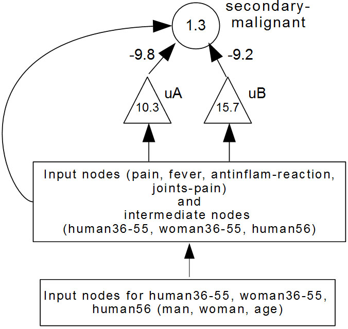

Due to inseparability, random cells need to be inserted among each of the three output cells and the corresponding inputs. The inputs to each output cell are its corresponding inputs as defined in the dependency information of the domain along with the corresponding random cells [29, 30]. Figure 2 graphically depicts the part of the connectionist knowledge base including the output cell ‘disease-type is secondary-malignant’, the two random cells and their corresponding inputs. Table 10 depicts in the form of a matrix the corresponding part of the connectionist knowledge base. The first row of the table depicts the names of intermediate and output cells whereas the first column depicts the names of input and intermediate cells. The names ‘Int. var1 (uA)’ and ‘Int. var1 (uB)’ correspond to random cells and have no meaning to the user.

Table 10

A part of a connectionist knowledge base depicted in the form of a matrix (corresponding to Fig. 2)

	Human-36-55	Woman-36-55	Human56	Int. var1 (uA)	Int. var2 (uB)	Secondary-malignant
Bias	$-$ 1.0	$-$ 2.1	$-$ 0.4	10.3	15.7	1.3
Man	3.1	0	2.8	0	0	0
Woman	3.3	1.2	2.7	0	0	0
Age $>$ 35	3.3	1.0	0	0	0	0
Age $<$ 56	3.1	1.1	0	0	0	0
Age $>$ 55	0	0	2.6	0	0	0
Pain-night	0	0	0	$-$ 0.3	$-$ 12.9	1.5
Pain-continuous	0	0	0	$-$ 4.6	0.8	0.8
Ant-reaction-none	0	0	0	$-$ 3.8	$-$ 12.8	5.2
Joints-pain-no	0	0	0	$-$ 3.9	1.5	1.5
Fever-no-fever	0	0	0	$-$ 0.6	$-$ 6.0	1.2
Human-36-55	0	0	0	$-$ 3.8	$-$ 9.2	1.6
Woman-36-55	0	0	0	$-$ 7.9	$-$ 2.5	1.1
Human56	0	0	0	$-$ 0.9	$-$ 13.5	0.9
Int. var1 (uA)	0	0	0	0	0	$-$ 9.8
Int. var2 (uB)	0	0	0	0	0	$-$ 9.2

The following two sections present alternative inference mechanisms for connectionist expert systems already introduced in literature and unexplored aspects involving them along with experimental results.

4.1 Alternative inference mechanisms for connectionist expert systems

Two alternative inference mechanisms for connectionist expert systems have been presented. These involve MACIE presented by Gallant in [29, 30] and the recency inference engine (RIE) presented by Ghalwash in [39]. Both inference mechanisms use a goal stack to store pursued goals and the working memory to store facts. For each intermediate/output cell, the known and remaining sums are recorded.

The main steps of these inference mechanisms are as follows. The user is asked to provide input data prior the beginning of inference and when necessary during inference. When the value of an input/intermediate cell becomes known during reasoning, the known and remaining sums of all affected cells in the knowledge base are updated accordingly. The goal stack and working memory are also updated. After updates are done and output goals remain in the goal stack, the mechanisms focus on a specific intermediate/output cell and pursue the corresponding goal (backward chaining). The two mechanisms differ in how to determine the cell for which backward chaining will be performed. For this purpose, MACIE uses the ‘confidence measure’ [29, 30] whereas RIE uses the ‘firing ratio’ [39]. These aspects will be explained in the following.

For cells with known outputs, the confidence measure is equal to their actual output. For unknown input cells, the confidence measure is equal to zero. The confidence measure for each unevaluated (intermediate or output) cell is computed based on the confidence measures of their inputs and the corresponding weights. More specifically, it is equal to the ratio of: (a) the sum of the product of the confidence measure of each input and the corresponding weight to (b) the sum of the absolute values of all input weights corresponding to cells whose value has not been determined. MACIE checks only the unevaluated output cells to find the one with the maximum absolute value of the confidence measure. Backward chaining is performed based on the specific output cell.

The firing ratio for each cell is defined as the ratio of the absolute value of the known sum to the remaining sum. All unevaluated intermediate and output cells are checked to find the one with the maximum firing ratio. Therefore, MACIE focuses only on output cells to start backward chaining whereas RIE focuses on both intermediate and output cells. The firing ratio may be computed independently for each cell whereas the confidence measure requires the computation of the confidence measures of all input cells.

The performance of MACIE and RIE were compared by Ghalwash in [39] using two small connectionist knowledge bases. The comparison was done in terms of the convergent rate. In [28], MACIE and RIE were compared in terms of the required computations to produce the output and the convergent rate. Six connectionist knowledge bases created from datasets and symbolic rule bases were used for this comparison. The set of input values used in these experiments was {1, $-$ 1, 0}. The experiments showed that RIE required fewer computations than MACIE in order to produce the output. This was due to the fact that the confidence measure used in MACIE resulted in computations not required in RIE. MACIE and RIE had the same performance in terms of the convergent rate in all but one knowledge base in which MACIE performed better. Note that the used knowledge bases were dense meaning that the output concepts depended on all or most of the input concepts. It should be mentioned that according to the discussion in [39], RIE performs clearly better than MACIE in case of sparse knowledge bases.

4.2 Unexplored aspects regarding the inference mechanisms of connectionist expert systems

In this section, various unexplored aspects regarding the reasoning mechanisms of connectionist expert systems are discussed. Corresponding experimental results are given. For these experiments, six connectionist knowledge bases were constructed following the procedure described in [29, 30]. Six corresponding datasets were used for these experiments. It should be mentioned that the same datasets were also used in [28] in the experiments involving MACIE and RIE. This enables a comparison with the results presented in this paper.

Two datasets were derived from the two medical rule bases used in the previous section. These datasets were created from training sets derived in the construction process of neurules from symbolic rules. More specifically, the training examples of the combined truth table for each intermediate/output conclusion were used [27].

A further dataset involves the acute dataset introduced in [29, 30]. The specific dataset involves six input variables, two intermediate conclusions and three output conclusions. The other three datasets are the lenses, car and nursery datasets from the Machine Learning repository [36]. For the car and nursery datasets dependency information provided by their donators was also used [40]. This facilitates the creation of the connectionist knowledge bases which is not a straightforward process. The knowledge bases for the car and nursery datasets using the dependency information are named ‘Car-dep’ and ‘Nursery-dep’ in the remaining part of this paper. The dependency information for the car dataset involves three intermediate variables each one taking four symbolic values. This results into twelve intermediate conclusions. The dependency information for the nursery dataset involves four intermediate variables. One of them takes four symbolic values whereas each one of the other three intermediate variables takes three symbolic values. This results into thirteen intermediate conclusions.

An unexplored aspect is to provide experimental results comparing MACIE and RIE for the alternative set of input values {1, 0, 0.5}. For this purpose, experiments were run for this set of input values. The connectionist knowledge bases were constructed using the {1, 0, 0.5} set of values. The inference mechanisms used this set of values to produce outputs.

Experimental results for the {1, 0, 0.5} set of values are presented in Tables 11 and 12. The initials “CKB” stand for connectionist knowledge base. The experimental results involve the mean number of required computations, the mean number of required inputs and the convergent rate. Computations involve the mean number of times that a product of a weight and a corresponding input value were added to the known (weighted) sum of a node The additional computations required in MACIE for the calculation of confidences are displayed besides the “ $+$ ” symbol in each case. The results show that RIE requires fewer computations to produce outputs as in the case of the {1, $-$ 1, 0} set of values [28]. Therefore, for the two alternative sets of values {1, $-$ 1, 0} and {1, 0, 0.5} it is verified that RIE requires less computations than MACIE to produce outputs. Comparing the corresponding results in [28] involving the {1, $-$ 1, 0} set of values and the results in Tables 11 and 12, it can be seen that more computations are required to produce outputs for the {1, 0, 0.5} set of values.

Table 11
Results for performance of MACIE (set {1, 0, 0.5})

CKB	Results
	Asked variables	Computations	Conv. rate
KB1	5.43	190.14 $+$ 110.83	0.934
KB2	5	668.10 $+$ 332.16	1
Acute	5.31	19.35 $+$ 15.92	0.732
Car-dep	5.83	242.57 $+$ 74.92	0.986
Lenses	3.67	48.92 $+$ 20.08	0.965
Nursery-dep	6.58	226.51 $+$ 80.25	0.973

Table 12

Results for performance of RIE (set {1, 0, 0.5})

CKB	Results
	Asked variables	Computations	Conv. rate
KB1	5.48	189.86	0.934
KB2	5	669	1
Acute	5.23	18.19	0.735
Car-dep	5.97	245.36	0.987
Lenses	3.71	46.17	0.966
Nursery-dep	7.22	220.18	0.963

The results concerning the convergent rate show that the performance of the two mechanisms is close. The convergent rate was computed using the number of given inputs and the number of input concepts in produced explanation rules. MACIE performs slightly better in one knowledge base. These results show that in certain cases, MACIE may perform better than RIE in terms of the convergent rate for the {1, 0, 0.5} set of values. In this aspect, the results are similar to the ones reported in [28] for the {1, $-$ 1, 0} set of values.

We run experiments for variations of MACIE to record how the performance is affected. To the best of our knowledge, four of these variations have not been mentioned by other researchers whereas the other one was mentioned in [29] but not tested.

As already mentioned, MACIE focuses on the output cells to find the one with the maximum confidence and then perform a type of backward chaining. Two variations were tested regarding the aforementioned aspect, that is, which cells will be checked to find the one with the maximum confidence. The former, named henceforth ‘MACIE-variation-1’, checks all unevaluated intermediate and output cells. The latter, named henceforth ‘MACIE-variation-2’, checks only the recently triggered intermediate and output cells. Therefore, MACIE-variation-2 resembles RIE but uses the confidence measure instead of the firing ratio.

Tables 13 and 14 provide results for MACIE-variation-1 and MACIE-variation-2, respectively for the {1, 0, 0.5} set of values. One may note that the results for MACIE and MACIE-variation-1 are close. MACIE-variation-1 requires slightly less computations in three knowledge bases (i.e., acute, lenses, nursery-dep) and slightly more computations in two knowledge bases (i.e., kb1, car-dep). In one knowledge base (i.e., kb2), the results are essentially the same. MACIE-variation-2 gives the same results as MACIE-variation-1 in four knowledge bases and almost the same results in the other two knowledge bases. Compared to MACIE, MACIE-variation-2 gives similar results as MACIE-variation-1. As far as the convergent rate is concerned, all three approaches provide almost the same results in five knowledge bases and in one knowledge base (i.e., kb1), MACIE is slightly better. Therefore, none of the three approaches outperforms the other two in all the knowledge bases. An interesting aspect is to compare the results for MACIE-variation-2 and RIE because MACIE-variation-2 resembles RIE. One may note that the results for these two methods are identical in four knowledge bases if the computations for the confidence measure are not taken into account. In the other knowledge bases, the results are very close for both methods.

Table 13

Results for performance of MACIE-variation-1 (set {1, 0, 0.5})

CKB	Results
	Asked variables	Computations	Conv. rate
KB1	5.76	194.24 $+$ 111.67	0.905
KB2	5	668.79 $+$ 332.92	1
Acute	5.23	18.19 $+$ 16.04	0.735
Car-dep	5.97	245.44 $+$ 75.79	0.987
Lenses	3.71	46.17 $+$ 20.29	0.966
Nursery-dep	7.22	220.18 $+$ 85.98	0.963

Table 14

Results for performance of MACIE-variation-2 (set {1, 0, 0.5})

CKB	Results
	Asked variables	Computations	Conv. rate
KB1	5.57	194.98 $+$ 114.74	0.923
KB2	5	668.79 $+$ 332.92	1
Acute	5.23	18.19 $+$ 16.04	0.735
Car-dep	5.97	245.36 $+$ 75.74	0.987
Lenses	3.71	46.17 $+$ 20.29	0.966
Nursery-dep	7.22	220.18 $+$ 85.98	0.963

Table 15

Results for performance of MACIE-variation-1 (set {1, $-$ 1, 0})

CKB	Results
	Asked variables	Computations	Conv. rate
KB1	5.07	177.14 $+$ 109.14	0.901
KB2	5	598.54 $+$ 313.58	1
Acute	4.59	17.48 $+$ 15.11	0.710
Car-dep	4.44	158.96 $+$ 68.26	0.987
Lenses	3.71	42.04 $+$ 18.67	0.944
Nursery-dep	6.48	197.70 $+$ 84.29	0.720

Table 16

Results for performance of MACIE-variation-2 (set {1, $-$ 1, 0})

CKB	Results
	Asked variables	Computations	Conv. rate
KB1	5.02	177.16 $+$ 108.93	0.910
KB2	5	598.54 $+$ 313.58	1
Acute	4.96	17.85 $+$ 15.19	0.660
Car-dep	4.47	159.40 $+$ 68.12	0.981
Lenses	3.71	42.04 $+$ 18.67	0.944
Nursery-dep	6.28	195.81 $+$ 83.08	0.720

Tables 15 and 16 provide results for MACIE-variation-1 and MACIE-variation-2, respectively for the {1, $-$ 1, 0} set of values. By comparing the results in these two tables and the results involving MACIE presented in [28], one may note that the results for all three approaches are close. None of them outperforms the others in all the knowledge bases. MACIE-variation-1 requires the same computations as MACIE in two knowledge bases (i.e., acute, lenses), essentially the same in one knowledge base (i.e., car-dep), slightly more in two knowledge bases (i.e., kb1 and nursery-dep) and slightly less in one knowledge base (i.e., kb2). MACIE-variation-2 gives essentially the same results as MACIE-variation-1 in five knowledge bases and slightly the same results in one knowledge base. The results are similar for the convergent rate.

A further variation of MACIE was mentioned but not tested in [29]. This involves the following aspect. As mentioned above, during inference MACIE checks the output cells to find the one with the maximum absolute value of the confidence measure. A variation is to examine the mere value of each confidence measure and not the absolute value. For this variation it is mentioned in [29] that the results will not be very different compared to the typical approach. This variation of MACIE will be henceforth named ‘MACIE-variation-3’. We run experiments for MACIE-variation-3 using the aforementioned six connectionist knowledge bases.

Table 17

Results for performance of MACIE-variation-3 (set {1, $-$ 1, 0})

CKB	Results
	Asked variables	Computations	Conv. rate
KB1	5.07	178.98 $+$ 102.23	0.937
KB2	5	589.01 $+$ 295.04	1
Acute	4.59	17.41 $+$ 15.81	0.710
Car-dep	4.32	156.43 $+$ 66.24	0.986
Lenses	3.71	42.04 $+$ 18.67	0.944
Nursery-dep	4.67	137.01 $+$ 66.55	0.980

Table 17 presents results for MACIE-variation-3 for the {1, $-$ 1, 0} set of values. One may note that compared to the performance of MACIE [28], the performance of MACIE-variation-3 is better in three knowledge bases (i.e., nursery-dep, car-dep, kb2), exactly the same in one knowledge base (i.e., lenses), roughly the same in one knowledge base (i.e., acute) and worse in one knowledge base (i.e., kb1). Compared to the performance of MACIE-variation-1 and MACIE-variation-2, the performance of MACIE-variation-3 is better in four knowledge bases (i.e., kb2, acute, car-dep and nursery-dep), the same in one knowledge base (i.e., lenses) and worse in one knowledge base (i.e., kb1). These results mean that MACIE-variation-3 is a more promising variation of MACIE compared to MACIE-variation-1 and MACIE-variation-2 for the {1, $-$ 1, 0}.

Table 18

Results for performance of MACIE-variation-3 (set {1, 0, 0.5})

CKB	Results
	Asked variables	Computations	Conv. rate
KB1	5.64	194.98 $+$ 113.69	0.928
KB2	5	659.57 $+$ 323.28	0.993
Acute	5.31	19.35 $+$ 15.92	0.732
Car-dep	5.83	241.64 $+$ 75.40	0.986
Lenses	3.67	48 $+$ 20.38	0.966
Nursery-dep	6.29	202.39 $+$ 80.11	0.978

Table 18 presents results for MACIE-variation-3 for the {1, 0, 0.5} set of values. Compared to the performance of MACIE, the performance of MACIE-variation-3 is better in two knowledge bases (i.e., kb2 and nursery-dep), the same in one knowledge base (i.e., acute), roughly the same in two knowledge bases (i.e., car-dep, lenses) and worse in one knowledge base (i.e., kb1). Compared to the performance of MACIE-variation-1 and MACIE-variation-2, the performance of MACIE-variation-3 is better in three knowledge bases (i.e., nursery-dep, car-dep, kb2), roughly the same in two knowledge bases (i.e., kb1, acute) and slightly worse in one knowledge base (i.e., lenses). Once again, from the results it seems that MACIE-variation-3 is a more promising variation of MACIE compared to MACIE-variation-1 and MACIE-variation-2.

The basic idea of MACIE-variation-3 may be used in combination with the main ideas of MACIE-variation-1 and MACIE-variation-2. Henceforth, MACIE-variation-1b and MACIE-variation-2b will be named the respective variations of MACIE. In MACIE-variation-1b, all intermediate/output cells will be checked to find the one with the maximum value of the confidence measure. In MACIE-variation-2b, the recently triggered cells will be examined to find the one with the maximum value of the confidence measure. We run experiments for MACIE-variation-1b and MACIE-variation-2b for both sets of input values.

Table 19

Results for performance of MACIE-variation-1b (set {1, $-$ 1, 0})

CKB	Results
	Asked variables	Computations	Conv. rate
KB1	5.25	175.80 $+$ 110.14	0.879
KB2	5	588.84 $+$ 294.04	1
Acute	4.59	17.48 $+$ 15.11	0.710
Car-dep	5.79	201.61 $+$ 75.84	0.789
Lenses	3.71	42.04 $+$ 18.67	0.944
Nursery-dep	6.21	190.95 $+$ 86.40	0.720

Table 19 presents results involving MACIE-variation-1b for the set of {1, $-$ 1, 0} values. Compared to the performance of MACIE-variation-1, the performance of MACIE-variation-1b is better in two knowledge bases (i.e., kb2, nursery-dep), exactly the same in two knowledge bases (i.e., acute, lenses), roughly the same in one knowledge base (i.e., kb1) and worse in one knowledge base (i.e., car-dep). The last finding (i.e., worse performance of MACIE-variation-1b in a knowledge base) is an interesting aspect. Compared to MACIE, MACIE-variation-1b requires exactly the same computations in acute and lenses knowledge bases, less computations in nursery-dep and kb2, slightly more computations in kb1 and clearly more computations in car-dep.

Table 20

Results for performance of MACIE-variation-1b (set {1, 0, 0.5})

CKB	Results
	Asked variables	Computations	Conv. rate
KB1	5.93	194.60 $+$ 116.05	0.892
KB2	5	668.10 $+$ 333.85	1
Acute	5.23	18.19 $+$ 16.04	0.735
Car-dep	5.83	242.36 $+$ 73.84	0.986
Lenses	3.67	48.92 $+$ 20.08	0.966
Nursery-dep	7.49	225.27 $+$ 82.11	0.964

Table 20 presents results involving MACIE-variation-1b for the set of {1, 0, 0.5} values. Compared to MACIE-variation-1, the results for MACIE-variation-1b are exactly the same in one knowledge base (i.e., acute), roughly the same in three knowledge bases (i.e., kb2, lenses, nursery-dep), slightly better in one knowledge base (i.e., car-dep) and slightly worse in one knowledge base (i.e., kb1).

Table 21

Results for performance of MACIE-variation-2b (set {1, $-$ 1, 0})

CKB	Results
	Asked variables	Computations	Conv. rate
KB1	5.23	175.52 $+$ 110.11	0.883
KB2	5	588.84 $+$ 294.04	1
Acute	4.59	17.37 $+$ 15.22	0.710
Car-dep	5.81	202.13 $+$ 76.43	0.793
Lenses	3.71	42.04 $+$ 18.67	0.944
Nursery-dep	6.14	192.21 $+$ 85.35	0.718

Table 21 presents results involving MACIE-variation-2b for the set of {1, $-$ 1, 0} values. Compared to MACIE-variation-2, the results are better in two knowledge bases (i.e., kb2, nursery-dep), exactly the same in one knowledge base (i.e., lenses) and roughly the same in two knowledge bases (i.e., kb1, acute).

Table 22

Results for performance of MACIE-variation-2b (set {1, 0, 0.5})

CKB	Results
	Asked variables	Computations	Conv. rate
KB1	5.88	193.60 $+$ 115.88	0.887
KB2	5	668.10 $+$ 333.85	1
Acute	5.46	19.69 $+$ 16.50	0.725
Car-dep	5.83	240.46 $+$ 73.14	0.986
Lenses	3.67	48.92 $+$ 20.08	0.966
Nursery-dep	7.49	225.27 $+$ 82.11	0.964

Table 22 presents results involving MACIE-variation-2b for the set of {1, 0, 0.5} values. Compared to MACIE-variation-2, the results are better in one knowledge base (i.e., car-dep), worse in one knowledge base (i.e., nursery-dep) and roughly the same in three knowledge bases (i.e., kb1, kb2, acute, lenses).

Table 23

Results for performance of all MACIE approaches (set {1, $-$ 1, 0})

CKB	Results
	Asked variables	Computations	Conv. rate
KB1 (MACIE)	5.27	172.43 $+$ 100.77	0.934
KB1 (MC-V1)	5.07	177.14 $+$ 109.14	0.901
KB1 (MC-V2)	5.02	177.16 $+$ 108.93	0.910
KB1 (MC-V3)	5.07	178.98 $+$ 102.23	0.937
KB1 (MC-V1B)	5.25	175.80 $+$ 110.14	0.879
KB1 (MC-V2B)	5.23	175.52 $+$ 110.11	0.883
KB2 (MACIE)	5	603.96 $+$ 310.16	1
KB2 (MC-V1)	5	598.54 $+$ 313.58	1
KB2 (MC-V2)	5	598.54 $+$ 313.58	1
KB2 (MC-V3)	5	589.01 $+$ 295.04	1
KB2 (MC-V1B)	5	588.84 $+$ 294.04	1
KB2 (MC-V2B)	5	588.84 $+$ 294.04	1
Acute (MACIE)	4.59	17.48 $+$ 15.11	0.709
Acute (MC-V1)	4.59	17.48 $+$ 15.11	0.710
Acute (MC-V2)	4.96	17.85 $+$ 15.19	0.660
Acute (MC-V3)	4.59	17.41 $+$ 15.19	0.710
Acute (MC-V1B)	4.59	17.48 $+$ 15.11	0.710
Acute (MC-V2B)	4.59	17.37 $+$ 15.22	0.710
Car-dep (MACIE)	4.44	158.05 $+$ 68.07	0.987
Car-dep (MC-V1)	4.44	158.96 $+$ 68.26	0.987
Car-dep (MC-V2)	4.47	159.40 $+$ 68.12	0.981
Car-dep (MC-V3)	4.32	156.43 $+$ 66.24	0.986
Car-dep (MC-V1B)	5.79	201.61 $+$ 75.84	0.789
Car-dep (MC-V2B)	5.81	202.13 $+$ 76.43	0.793
Lenses (MACIE)	3.71	42.04 $+$ 18.67	0.944
Lenses (MC-V1)	3.71	42.04 $+$ 18.67	0.944
Lenses (MC-V2)	3.71	42.04 $+$ 18.67	0.944
Lenses (MC-V3)	3.71	42.04 $+$ 18.67	0.944
Lenses (MC-V1B)	3.71	42.04 $+$ 18.67	0.944
Lenses (MC-V2B)	3.71	42.04 $+$ 18.67	0.944
Nursery-dep (MACIE)	6.06	195.50 $+$ 84.18	0.733
Nursery-dep (MC-V1)	6.48	197.70 $+$ 84.29	0.720
Nursery-dep (MC-V2)	6.28	195.81 $+$ 83.08	0.718
Nursery-dep (MC-V3)	4.67	137.01 $+$ 66.55	0.980
Nursery-dep (MC-V1B)	6.21	190.95 $+$ 86.40	0.720
Nursery-dep (MC-V2B)	6.14	192.21 $+$ 85.35	0.718

Table 23 presents results involving all MACIE approaches for the set of {1, $-$ 1, 0} values. The initials ‘MC-V’ stand for ‘MACIE-variation’. Results shown in italics correspond to the best ones for the specific knowledge bases. The results for lenses are exactly the same and are not highlighted. Multiple instances that correspond to the best result in a single knowledge base are also not highlighted. On average, one may note that MACIE-variation-3 gives better results than the other approaches. More specifically, as far as the mean number of computations is concerned, MACIE-variation-3 gives the best results in three knowledge bases and in two other knowledge bases its performance is very close to the best ones. Furthermore, in all knowledge bases, MACIE-variation-3 gives the best results as far as the convergent rate is concerned. As far as the mean number of asked variables is concerned, MACIE-variation-3 gives the best results in five knowledge bases (i.e., kb2, acute, car-dep, lenses, nursery-dep) and is very close to the best result in the other knowledge base (i.e., kb1).

Table 24

Average results for all MACIE approaches (set {1, $-$ 1, 0})

CKB	Average results
	Asked variables	Computations	Conv. rate
MACIE	4.85	198.24 $+$ 99.49	0.885
MC-V1	4.88	198.64 $+$ 101.51	0.877
MC-V2	4.91	198.47 $+$ 101.26	0.869
MC-V3	4.56	186.81 $+$ 93.99	0.926
MC-V1B	5.09	202.79 $+$ 100.03	0.840
MC-V2B	5.08	203.02 $+$ 99.97	0.841

Table 24 presents the average results for all MACIE approaches for the {1, $-$ 1, 0} set of values. MACIE-variation-3 gives the best results followed by MACIE-variation-2.

Table 25

Results for performance of all MACIE approaches (set {1, 0, 0.5})

CKB	Results
	Asked variables	Computations		Conv. rate
KB1 (MACIE)	5.43	190.14	$+$ 110.83	0.934
KB1 (MC-V1)	5.76	194.24	$+$ 111.67	0.905
KB1 (MC-V2)	5.57	194.98	$+$ 114.74	0.923
KB1 (MC-V3)	5.64	194.98	$+$ 113.69	0.928
KB1 (MC-V1B)	5.93	194.60	$+$ 116.05	0.892
KB1 (MC-V2B)	5.88	193.60	$+$ 115.88	0.887
KB2 (MACIE)	5	668.10	$+$ 332.16	1
KB2 (MC-V1)	5	668.79	$+$ 332.92	1
KB2 (MC-V2)	5	668.79	$+$ 332.92	1
KB2 (MC-V3)	5	659.57	$+$ 323.28	0.993
KB2 (MC-V1B)	5	668.10	$+$ 333.85	1
KB2 (MC-V2B)	5	668.10	$+$ 333.85	1
Acute (MACIE)	5.31	19.35	$+$ 15.92	0.732
Acute (MC-V1)	5.23	18.19	$+$ 16.04	0.735
Acute (MC-V2)	5.23	18.19	$+$ 16.04	0.735
Acute (MC-V3)	5.31	19.35	$+$ 15.92	0.732
Acute (MC-V1B)	5.23	18.19	$+$ 16.04	0.735
Acute (MC-V2B)	5.46	19.69	$+$ 16.50	0.725
Car-dep (MACIE)	5.83	242.57	$+$ 74.92	0.986
Car-dep (MC-V1)	5.97	245.44	$+$ 75.79	0.987
Car-dep (MC-V2)	5.97	245.36	$+$ 75.74	0.987
Car-dep (MC-V3)	5.83	241.64	$+$ 75.40	0.986
Car-dep (MC-V1B)	5.83	242.36	$+$ 73.84	0.986
Car-dep (MC-V2B)	5.83	240.46	$+$ 73.14	0.986
Lenses (MACIE)	3.67	48.92	$+$ 20.08	0.965
Lenses (MC-V1)	3.71	46.17	$+$ 20.29	0.966
Lenses (MC-V2)	3.71	46.17	$+$ 20.29	0.966
Lenses (MC-V3)	3.67	48	$+$ 20.38	0.966
Lenses (MC-V1B)	3.67	48.92	$+$ 20.08	0.966
Lenses (MC-V2B)	3.67	48.92	$+$ 20.08	0.966
Nursery-dep (MACIE)	6.58	226.51	$+$ 80.25	0.973
Nursery-dep (MC-V1)	7.22	220.18	$+$ 85.98	0.963
Nursery-dep (MC-V2)	7.22	220.18	$+$ 85.98	0.963
Nursery-dep (MC-V3)	6.29	202.39	$+$ 80.11	0.978
Nursery-dep (MC-V1B)	7.49	225.27	$+$ 82.11	0.964
Nursery-dep (MC-V2B)	7.49	225.27	$+$ 82.11	0.964

Table 25 presents results involving all MACIE approaches for the set of {1, 0, 0.5} values. The picture is not clear as in the case of the results involving the {1, $-$ 1, 0} set of values. As far as the mean number of computations is concerned, MACIE gives the best results in one knowledge base (i.e., kb1), MACIE-variation-3 in two knowledge bases (i.e., kb2, nursery-dep), MACIE-variation-1 and MACIE-variation-2 in two knowledge bases (i.e., acute, lenses) and MACIE-variation-2b in one knowledge base.

Table 26

Average results for all MACIE approaches (set {1, 0, 0.5})

CKB	Average results
	Asked variables	Computations	Conv. rate
MACIE	5.30	232.60 $+$ 105.69	0.932
MC-V1	5.48	232.17 $+$ 107.12	0.926
MC-V2	5.45	232.28 $+$ 107.62	0.929
MC-V3	5.29	227.66 $+$ 104.80	0.931
MC-V1B	5.53	232.91 $+$ 107.00	0.924
MC-V2B	5.56	232.67 $+$ 106.93	0.921

Table 26 presents the average results for all MACIE approaches for the {1, 0, 0.5} set of values. On average, MACIE-variation-3 gives the best results for mean number of computations and mean asked inputs followed by MACIE. On average, MACIE gives the best result for the convergent rate closely followed by MACIE-variation-3. The average performance of MACIE-variation-3 is affected by its performance in nursery-dep in which it clearly outperforms the other approaches.

5. Conclusions

This paper discusses aspects regarding the reasoning mechanisms of neurules and connectionist expert systems. These aspects had not been previously explored. More specifically, the order of each neurule is adjusted according to the number of symbolic rules or training examples constituting its source knowledge. This plays a role in conflict resolution during backward chaining. The experimental results show that the performance of the reasoning mechanism is improved.

As far as connectionist expert systems are concerned, five variations of MACIE are explored. More specifically, two variations are presented in this work for the first time. The third one was mentioned in [29] without providing experimental results. The fourth and fifth variations, also presented in this work for the first time, combine the ideas of the first two variations and the third one. To the best of our knowledge, the four of the five variations have not been mentioned in the work of other researchers whereas the other one was mentioned and not tested in previous work.

The experiments showed that none of the alternative versions of MACIE outperforms the others in all cases. However, the third variation performs better than the others in most cases. The experiments were performed using two alternative set of values (i.e., {1, $-$ 1, 0} and {1, 0, 0.5}). Furthermore, results for the alternative set of {1, 0, 0.5} values are given comparing RIE [39] and MACIE [29, 30]. The previous comparison of these two mechanisms was based on results using the {1, $-$ 1, 0} set of values [28].

There are two main directions for future research. One direction concerns the use of combined intelligent approaches in medicine. Combined approaches may be used in various medical domains due to the existence of symbolic and empirical knowledge. The other direction concerns the use of combined intelligent approaches in the construction of an intelligent educational system addressed to early childhood. Few intelligent educational systems addressed to early childhood have been developed [41]. Combined intelligent approaches satisfy the knowledge representation requirements of intelligent educational systems [42, 43].

References

Medsker

. Hybrid intelligent systems. 2nd Printing. Dordrecht: Kluwer Academic Publishers; 1998.

Hatzilygeroudis

Perikos

Grivokostopoulou

, eds. Advances in integrations of intelligent methods, Smart Innovations, Systems and Technologies, vol. 170. Singapore: Springer; 2020. doi: 10.1007/978-981-15-1918-5.

Melin

Castillo

Kacprzyk

, eds. Recent advances of hybrid intelligent systems based on soft computing, Studies in Computational Intelligence, vol. 915. Cham: Springer. doi: 10.1007/978-3-030-58728-4.

Bhoi

Mallick

Mohanty

de Albuquerque

VHC

. Hybrid Artificial Intelligence and IoT in healthcare, Intelligent Systems Reference Library, vol. 209. 2021; Singapore: Springer Nature. doi: 10.1007/978-981-16-2972-3.

Hatzilygeroudis

Prentzas

. Neuro-symbolic approaches for knowledge representation in expert systems. Int. J. Hybrid Intell. Syst.2004; 1(3–4): 111–126. doi: 10.3233/HIS-2004-13-401.

Sarker

Zhou

Eberhart

Hitzler

. Neuro-symbolic artificial intelligence. AI Commun. (in press). doi: 10.3233/AIC-210084.

Sitton

Alonso

Hernandez-Nieves

Rodriguez-Gonzalez

. Neuro-symbolic hybrid systems for Industry 4.0: A systematic mapping study. In: Uden

Ting

Corchado

, eds. Proceedings of the 14th International Conference on Knowledge Management Organizations, Communications in Computer and Information Science, vol. 1027. Cham: Springer; 2019, pp. 455–465. doi: 10.1007/978-3-030-21451-7_39.

Nauck

Klawonn

Kruse

. Foundations of neuro-fuzzy systems. New York: John Wiley & Sons; 1997.

de Campos Souza

. Fuzzy neural networks and neuro-fuzzy networks: A review the main techniques and applications used in the literature. Appl. Soft Comput.2020; 92: 106275. doi: 10.1016/j.asoc.2020.106275.

10.

Shihabudheen

Pillai

. Recent advances in neuro-fuzzy system: A survey. Knowl Based Syst.2018; 152: 136–162. doi: 10.1016/j.knosys.2018.04.014.

11.

Tang

Wang

Tao

. Fouling potential prediction and multi-objective optimization of a flue gas heat exchanger using neural networks and genetic algorithms. Int. J. Heat Mass Transf.2020; 152: 119488. doi: 10.1016/j.ijheatmasstransfer.2020.119488.

12.

Liu

Zhang

Zhao

Wang

Sun

. Neural network control system of cooperative robot based on genetic algorithms. Neural. Comput. Appl.2021; 33: 8217–8226. doi: 10.1007/s00521-020-04952-1.

13.

Nguyen

Kim

. Genetic convolutional neural network for intrusion detection systems. Future Gener. Comput. Syst.2020; 113: 418–427. doi: 10.1016/j.future.2020.07.042.

14.

Hamamoto

Carvalho

Sampaio

LDH

Abrao

Proenca Jr

. Network anomaly detection system using genetic algorithm and fuzzy logic. Expert Syst. Appl.2018; 92: 390–402. doi: 10.1016/j.eswa.2017.09.013.

15.

Gola

Kłosowski

. Development of computer-controlled material handling model by means of fuzzy logic and genetic algorithms. Neurocomputing.2019; 338: 381–392. doi: 10.1016/j.neucom.2018.05.125.

16.

Varzaneh

Rafsanjani

. Intrusion detection system using a new fuzzy rule-based classification system based on genetic algorithm. Intell. Decis. Technol.2021; 15(2): 231–237. doi: 10.3233/IDT-200036.

17.

Beligiannis

Hatzilygeroudis

Koutsojannis

Prentzas

. A GA driven intelligent system for medical diagnosis. In: Gabrys

Howlett

Jain

, eds. Proceedings of the 10th International Conference on Knowledge-Based Intelligent Information and Engineering Systems, Lecture Notes in Artificial Intelligence, vol. 4251. Heidelberg: Springer; 2006, pp. 968–975. doi: 10.1007/11892960_116.

18.

Jaithunbi

Sabena

SaiRamesh

. Trust evaluation of public cloud service providers using genetic algorithm with intelligent rules. Wirel. Pers. Commun. (in press). doi: 10.1007/s11277-021-08876-4.

19.

Ospina-Mateus

Jiménez

LAQ

Lopez-Valdes

Garcia

Barrero

Sana

. Extraction of decision rules using genetic algorithms and simulated annealing for prediction of severity of traffic accidents by motorcyclists. J. Ambient Intell. Humaniz. Comput. 2021; 10051–10072. doi: 10.1007/s12652-020-02759-5.

20.

Prentzas

Hatzilygeroudis

. Combinations of case-based reasoning with other intelligent methods. Int. J. Hybrid Intell. Syst.2009; 6(4): 189–209. doi: 10.3233/HIS-2009-0096.

21.

Prentzas

Hatzilygeroudis

. Assessment of life insurance applications: An approach integrating neuro-symbolic rule-based with case-based reasoning. Expert Syst.2016; 33: 145–160. doi: 10.1111/exsy.12137.

22.

Zaranezhad

Mahabadi

Dehghani

. Development of prediction models for repair and maintenance-related accidents at oil refineries using artificial neural network, fuzzy system, genetic algorithm, and ant colony optimization algorithm. Process Saf Environ Prot.2019; 131: 331–348. doi: 10.1016/j.psep.2019.08.031.

23.

Zhang

Liu

Rao

Zhao

. Optimal design of building environment with hybrid genetic algorithm, artificial neural network, multivariate regression analysis and fuzzy logic controller. Build Environ.2020; 175: 106810. doi: 10.1016/j.buildenv.2020.106810.

24.

Wang

Gao

. Parallel conjugate gradient-particle swarm optimization and the parameters design based on the polygonal fuzzy neural network. J. Intell. Fuzzy Syst.2019; 37(1): 1477–1489. doi: 10.3233/JIFS-182882.

25.

Varela-Santos

Melin

. A new modular neural network approach with fuzzy response integration for lung disease classification based on multiple objective feature optimization in chest X-ray images. Expert Syst. Appl.2021; 168: 114361. doi: 10.1016/j.eswa.2020.114361.

26.

Prado

Minutolo

Kristjanpoller

. Forecasting based on an ensemble autoregressive moving average-adaptive neuro-fuzzy inference system-neural network-genetic algorithm framework. Energy.2020; 197: 117159. doi: 10.1016/j.energy.2020.117159.

27.

Hatzilygeroudis

Prentzas

. Neurules: Improving the performance of symbolic rules. Int J Artif Intell Tools.2000; 9(1): 113–130. doi: 10.1142/S0218213000000094.

28.

Hatzilygeroudis

Prentzas

. Integrated rule-based learning and inference. IEEE Trans Knowl Data Eng.2010; 22(11): 1549–1562. doi: 10.1109/TKDE.2010.79.

29.

Gallant

. Connectionist expert systems. Commun. ACM.1988; 31(2): 152–169. doi: 10.1145/42372.42377.

30.

Gallant

. Neural network learning and expert systems. Boston: MIT Press; 1993.

31.

Prentzas

Hatzilygeroudis

. Exploring Aspects of Reasoning in NeuroSymbolic Rules and Connectionist Expert Systems. In: Proceedings of the 12th International Conference on Information, Intelligence, Systems and Applications. IEEE; 2021. doi: 10.1109/IISA52424.2021.9555527.

32.

Hatzilygeroudis

Prentzas

. Symbolic-neural rule based reasoning and explanation. Expert Syst. Appl.2015; 42: 4595–4609. doi: 10.1016/j.eswa.2015.01.068.

33.

Lucas

van der Gaag

. Principles of expert systems. Chatham: Addison-Wesley Publishers; 1991.

34.

Forgy

. OPS5 User’s Manual, Report No. CMU-CS-81-135. Pittsburg: Carnegie Mellon University; 1981.

35.

Russell

Norvig

. Artificial Intelligence: A modern approach. 4th ed. Hoboken: Pearson; 2020.

36.

UCI Machine Learning Repository [http://archive.ics.uci.edu/ml]. Irvine: University of California, School of Information and Computer Science; 2019. Available from: http://archive.ics.uci.edu/ml.

37.

Prentzas

Hatzilygeroudis

. Using clustering algorithms to improve the production of symbolic-neural rule bases from empirical data. Int J Artif Intell Tools.2018; 27: 1850002-1–1850002-36. doi: 10.1142/S0218213018500021.

38.

Hatzilygeroudis

Prentzas

. HYMES: A HYbrid Modular Expert System with efficient inference and explanation. In: Manolopoulos

Evripidou

, eds. Proceedings of the 8th Panhellenic Conference on Informatics. Athens: Antonis Livanis Publications; 2001, pp. 422–431.

39.

Ghalwash

. A recency inference engine for connectionist knowledge bases. Appl. Intell.1998; 9(3): 201–215. doi: 10.1023/A:1008311702940.

40.

Car and nursery datasets with concept hierachy. Ljubljana: Faculty of Computer and Information Science, University of Ljubljana; 1997. Available from: https://file.biolab.si/biolab/app/hint/datasets.html.

41.

Prentzas

. Artificial Intelligence methods in early childhood education. In: Yang

S-X

, ed. Artificial Intelligence, Evolutionary Computation and Metaheuristics, Studies in Computational Intelligence, vol. 427. Heidelberg: Springer-Verlag; 2013, pp. 169–199. doi: 10.1007/978-3-642-29694-9_8.

42.

Hatzilygeroudis

Prentzas

. Knowledge representation in intelligent educational systems. In: Ma

, ed. Web-based intelligent e-learning systems: Technologies and applications. Hershey: IGI Global; 2006, pp. 175–192. doi: 10.4018/978-1-59140-729-4.ch009.

43.

Prentzas

Hatzilygeroudis

Koutsojannis

. A Web-based ITS controlled by a hybrid expert system. In: Okamoto

Hartley

, Kinshuk Klus

, eds. Proceedings of the IEEE International Conference on Advanced Learning Technologies. New York: IEEE Computer Society; 2001, pp. 239–240. doi: 10.1109/ICALT.2001.943910.

Neurules and connectionist expert systems: Unexplored neuro-symbolic reasoning aspects

Abstract

Keywords

1. Introduction

2. Neurules

Table 2 Neurules produced from the symbolic rules in the example

4.2 Unexplored aspects regarding the inference mechanisms of connectionist expert systems

Table 11 Results for performance of MACIE (set {1, 0, 0.5})

References

Table 2
Neurules produced from the symbolic rules in the example

Table 11
Results for performance of MACIE (set {1, 0, 0.5})