
Abstract
This study performed a comparative analysis of various imputations for NULL values in the dataset, namely, mean, median, and mode. We implemented eleven regression models, including Linear and Support Vector Regression and tree-based regression models, such as decision tree, Surrogate tree, and random forest, with five different pre-processing techniques, providing different types of results. The core objective of this study is to compare these results and reach an interpretation as to why certain imputation technique produces a certain output. The interpretation of this result is helpful in the selection of the regression model. The experimental results of the proposed technique were evaluated and validated for the performance and quality analysis of life expectancy prediction using various quality parameters. Among the results, the highest accuracy was produced by random forest regression with an accuracy of 96.8%, which proves the significance of random forest in comparison to other state-of-the-art regression methods for life expectancy prediction.
Keywords
Introduction
Life Expectancy is a measure of how long a person can live under certain conditions [1,2]. These conditions include several socio-economic factors such as BMI, Income composition, schooling, and status of development [3,4,5]. Usually, developed countries tend to have higher life expectancies than developing or underdeveloped countries. The global average life expectancy of human beings has been rising, indicating that standards of living are improving and the mortality rate of diseases has been decreasing day by day [6,7,8,9]. Life expectancy also acts as an important indicator of how well the region’s population is doing in terms of social and economic development [10,11].
Regression models are used in various fields of research such as medicine, engineering, and economics to predict continuous values by establishing relationships between several variables. The accuracy of a model also depends on the data used for its training, and the quality of pre-processing techniques also plays a major role in the outcome of the model [12,13,14]. These data can be improved by replacing the NULL values with the mean, median, mode, and interpolation, or by completely dropping them. This study aimed to determine how algorithms respond to various pre-processing techniques by analyzing their impact on target life expectancy predictions [15,16]. This will help in determining the appropriate pre-processing techniques for specific algorithms [17].
The evaluation criteria to understand each result is to record their error metrics to determine the extent of error and problems arising while running statistical models, such as underfitting, overfitting, and other problems that might generate wrong results. Since different pre-processing techniques can result in different results in each model, understanding what techniques work best on an algorithm becomes essential. Some hyper-parameter changes were also made via trial and error for further improvement in results.
The outcome of this study can enhance our cognition about what factors severely impact life expectancy, and this information could be used to develop the standard of living further. We will also understand what regression methods give the best result and why. We have also tracked various performance metrics to understand how the model behaves with different inputations. We conclude that the Random Forest model has the best outcome compared to Linear Regression and Support Vector regression.
The paper briefs, as illustrated, are the literature review discussed in Section 2, materials and method in Section 3, results and discussion in Section 4, and finally, Section 5, which gives the conclusion and future scope of the proposed system.
Litearture review
In a study by Bali et al. [18] to find out suitable model for predicting Life Expectancy they used techniques such as ridge regression, linear regression, random forest, and decision tree regression. The NaN values were replaced with 0 and the fields ‘country’ and ‘year’ were dropped, as they did not analyze a specific country’s data. In their findings, Random Forest Regression performed the best, with an accuracy of 96%.
Another study by Lipesa et al. [10] implemented XGBoost, Random Forest, and Artificial Neural Networks. Their findings were analyzed based on the MAE and RMSE values. The best-performing model was XGBoost with an MAE of 1.554 and an RMSE of 2.402. The data used for this study were obtained from the World Health Organization (WHO). However, some of the data were found to be incorrect and were then replaced by new values taken from the development indicators’ dataset from the World Bank. Kavitha et al. [19] presented a comparison between ‘linear regression’ and ‘support vector regression’. They used different kernels for SVM, namely, linear and non-linear support vector regression. In this study, linear regression with the least squares method performed better than SVM.
Aydin and Bulut [20] used even more kernels in the support vector regression (SVR) namely, radial basis, linear, polynomial, and sigmoid functions. They use data from 32 countries and compared the results using graphical methods. Ali et al. [21] utilized additional algorithms and models, such as the classification model, recursive feature elimination, logistic regression model, and cirrhosis mortality model, to predict the life expectancy of people suffering from Hepatitis B. The Area Under-curve method was used to assess the model’s performance.
In a recent study by Tuj et al. [22] to find out the best accurate regression model they used 8 different types of techniques which include models like “K-neighbors”, “Stacking Regressor”, “Random Forest”, “Decision Tree”. The most accurate result was obtained by an extreme gradient boosting regressor with an accuracy of 99%, followed by gradient boosting, which produced an accuracy of 96%. For change, they separately collected data from rural and urban sources [23].
Several techniques were applied on a WHO dataset which includes “Linear Regression”, “Decision Tree” and “K-neighbour Regression” along with Correlation Features Selection and Mutual Information Features Selection methods to get the desired result i.e., of R2 and RMSE. The Decision Tree produced the best results with mutual information features producing the best result and correlation feature selection had a k values of 15 and 10 respectively [24].
A study by Lakshmanrao et al. [25] examined the feasibility of life expectancy on a WHO dataset of 15 years by applying machine-learning models. In this study, they applied logistic regression, SVM, random forest, and decision tree to achieve a good r-squared value of 0.81 by Multiple Linear Regression, 0.56 by Support Vector Regression, 0.91 by Decision Tree, and 0.96 by Random Forest.
In a study conducted by Faisal et al. [26], the WHO dataset was used to identify statistically significant factors for life expectancy using machine-learning models. Random Forest regression and Linear regression models were used. Furthermore, they used an ensemble voting regressor and a decision tree. In the results, it was found that schooling has a positive impact of 0.71, and the best model was the Random Forest regressor, which achieved the lowest MSE of 1.93, and the lowest MAE of 1.24.
Fransiska et al. [27] used geographically weighted regression (GWR) and Random Forest Regression (RFR) to compare life expectancy prediction with RMSE, the RMSE value of GWR was found to be 64.99 with significant influence variables X3 (percentage of proper sanitation households), X5 (number of doctors), and X7 (average years of schooling) denoting several socio-economic statistical values. The RMSE of the RFR was found to be 84.04 with significant influence variables X3, X5, and X7.
In a recent study by Yifan Wang [28], to find the strongest factors that affect life expectancy across several countries and continents, 24 different variables were considered from 2000 to 2015 in nearly 200 countries and six continents. Various factors include the Adult Mortality Rate, Income, and HIV/AIDS. North America was found to be the least affected by these factors, while Asia was found to be the most affected. On Applying the Random Forest Model, it was found that every continent has different affecting factors: the XGboost model had the lowest SHAP value in the regions of Haiti in North America and Sierra Leone in Africa, with Life Expectancy below 42 years, and the highest SHAP values were found for Canada, Germany, and Ireland, with an average life of 80 years and above.
In conclusion, HIV/AIDS was found to be negatively correlated with income and adult mortality, more schooling, higher SHAP values, higher income, and lower adult mortality. Xinyang He et al. [29] performed a recent study to find out the factors Affecting Life Expectancy, they considered the “Multiple Linear Regression” model to predict Life Expectancy. 18 Different factors are considered in the regression model, such as GDP, Schooling, Disease, etc.
When applying the MLR Model it was found that Disease, Income, and Schooling were the most influential factors, with an RMSE of 3.818. Furthermore, they bifurcated their study into two parts, developing nations, and developed nations, and found that for developing nations the most important factors were medical and schooling, and the RMSE was 3.99, for developed nations, the RMSE was 2.57.
The gap identified was that pre-processing techniques were not mentioned in some studies. In addition, one of the studies [18] replaced NULL values with 0. Considering real-life parameters, such as Adult Mortality and BMI to be zero, is unrealistic.
Therefore, the need for a study to perform an extensive comparative analysis across various models and pre-processing techniques was identified to understand how different models behave based on different imputations.
This study has been done with eleven different algorithms namely ‘Linear Regression (LR)’, ‘Support Vector Regression (SVR)’, ‘Random Forest (RF)’, ‘Decision Tree (DT)’, ‘Polynomial Regression (POLY)’, ‘Logistic Regression (LOGI)’, ‘Principal Regression (PRIN)’, ‘Gradient Boosting (GB)’, ‘Surrogate Tree (ST)’, ‘Ridge Regression (RIDG)’, and Multi-Layer Perceptron (MLP) Regressor’, and five different pre-processing techniques which lead to 40 different combinations of results.
Each result was evaluated based on several error metrics to analyze the extent of error, under-fitting, over-fitting, and other problems that can lead to inaccurate predictions by the model. As each error metric has a different behavior from pre-processing changes, it is important to analyze how it behaves to fine-tune the model properly to find the best pre-processing technique for each algorithm. Specific hyper-parameters were changed using the trial-and-error method to further improve the results.
Materials and methods
Dataset’s composition used in the study.
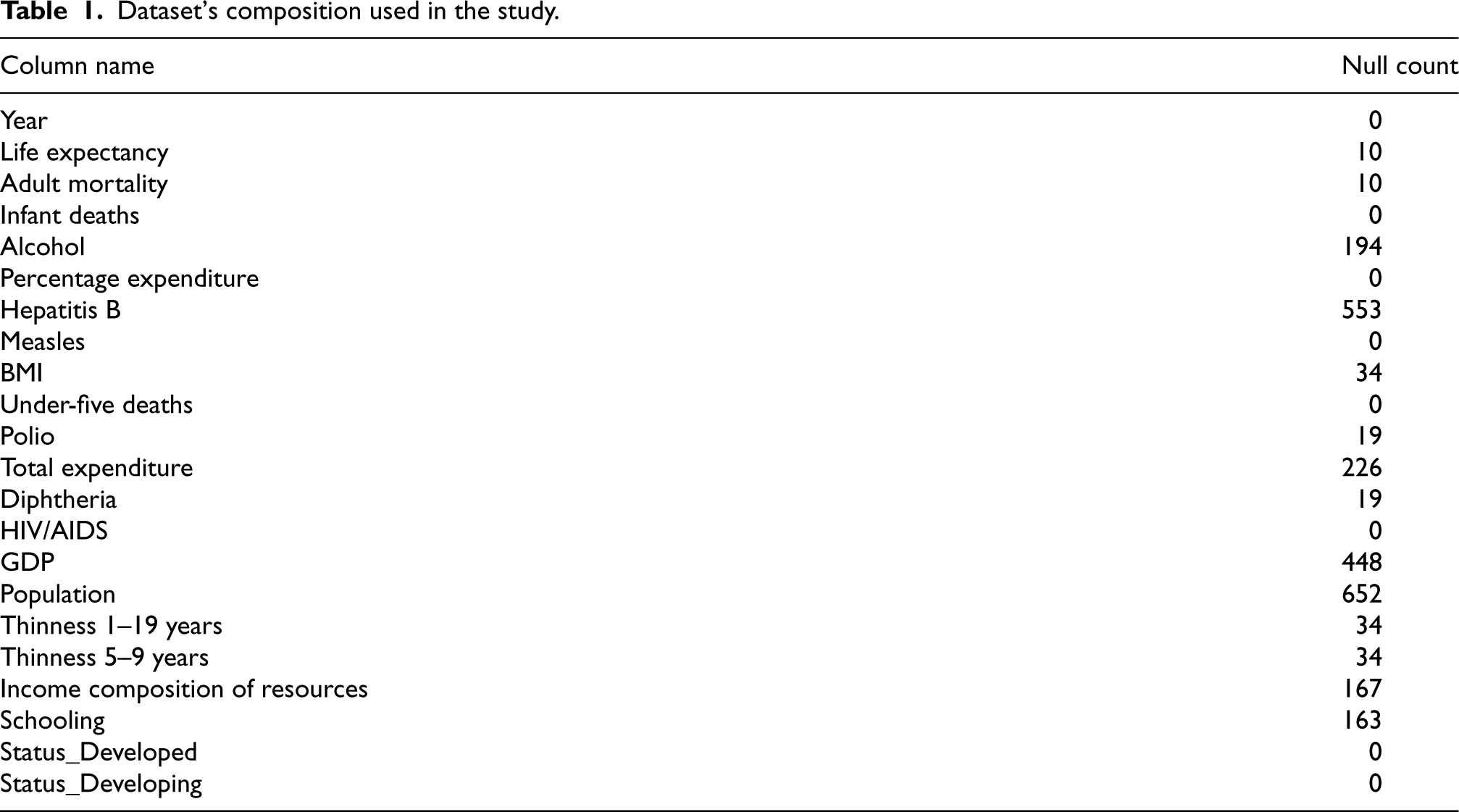
Dataset’s composition used in the study.
The dataset utilized in the study consisted of 22 columns, including life expectancy. Most variables (20 out of 22) were continuous data, while the categorical ‘Status’ column indicated whether a country was ‘Developed’ or ‘Developing.’ This categorical column was divided into two separate binary classification columns. As a result, the dataset contained 22 columns, with 20 having continuous values and 2 representing binary classification. The data was sourced from Kaggle [30], and Table 1 provides a detailed breakdown of the dataset’s composition utilized in this study.
The techniques used in this study were ‘Linear Regression (LR)’, ‘Support Vector Regression (SVR)’, ‘Random Forest (RF)’, ‘Decision Tree (DT)’, ‘Polynomial Regression (POLY)’, ‘Logistic Regression (LOGI)’, ‘Principal Component Regression (PRIN)’, ‘Gradient Boosting (GB)’, ‘Surrogate Tree (ST)’, ‘Ridge Regression (RIDG)’, and Multi-Layer Perceptron (MLP) Regressor’. The following is a brief description of the aforementioned techniques.
Linear regression is an approach for establishing a relationship between dependent and independent variables. There are two types of linear regression: simple linear regression, with only one independent variable to establish the relationship, and multiple linear regression, with two or more independent variables that contribute to establishing the relationship. The model tries to fit a straight line across data points that best represents the relationship possible.
Support vector regression
Support Vector Machine is a supervised ML algorithm that uses both regression and classification models. It aims to create the best line or decision boundary called a hyperplane, which uses extreme points or vectors to create the hyperplane. The upper boundary line is called a positive hyperplane and the lower one is called a negative hyperplane. There are two types of SVM: linear and non-linear. Linear SVM is used on datasets that can be classified into two parts by using a single straight line, whereas non-linear SVM is used whenever the data are non-separable by a single straight line.
Decision tree regression
A Decision Tree is a flowchart-like structure comprising nodes and branches. The internal node represents the attribute, the leaf node represents the label of the class, and the branch represents the outcome. It Works by splitting the data recursively into subsets based on the most significant features at each node.
Random forest regression
Random Forest is a machine-learning algorithm that works on training, testing, and prediction principles. It starts by creating multiple subsets of the dataset using bootstrapping then creates separate decision trees for each subset of the original data, and then combines all these decision trees to provide a more accurate prediction in the training part, creating subsets of the original dataset, and creating separate decision trees for each subset in testing by averaging the decision trees and then providing the most votes prediction. It is an ensemble model that uses two different methods: bagging, in which it creates different training subsets of original data for training the model, and boosting, in which it combines the weak learner with strong learners by creating a sequential model such as ADAboost, and XGboost. ADAboost, XGboost, etc.
Polynomial regression
Polynomial regression establishes a non-linear relationship between variables that are modelled in the form of an n-degree polynomial, where, n is a positive integer. The non-linear nature of polynomial regression helps provide flexibility to provide a better interpretation between the dependent values and their explanatory variables.
Principal component regression
This technique combines multiple linear regression and principal component analysis (PCA). This technique transforms the actual explanatory variables into linearly non-correlated values called principal components. These values are then ordered based on their ability to explain the outcome, which in this study was Life Expectancy. These values are arranged in descending order of their ability to explain the outcomes. Multiple linear regression analysis was performed by selecting the preferred number of components for use.
Logistic regression
Logistic Regression is designed to predict binary outcomes or outcomes divided into categories. It is not useful to predict continuous values using this algorithm; however, the task can be performed by transforming the problem into a classification task. After producing the outcome for some data, the outcome can be used to classify the results and calculate the weighted average of life expectancy for that particular task. Thus we could predict continuous values using logistic regression.
Gradient boosting regression
The gradient boosting model creates a strong model by using several weak models. In general, these weak models are usually decision trees; however, any algorithm can be used. A residual, that is, the difference between the actual and predicted values was used to train the weak models, and gradient descent was used to improve the model in each iteration.
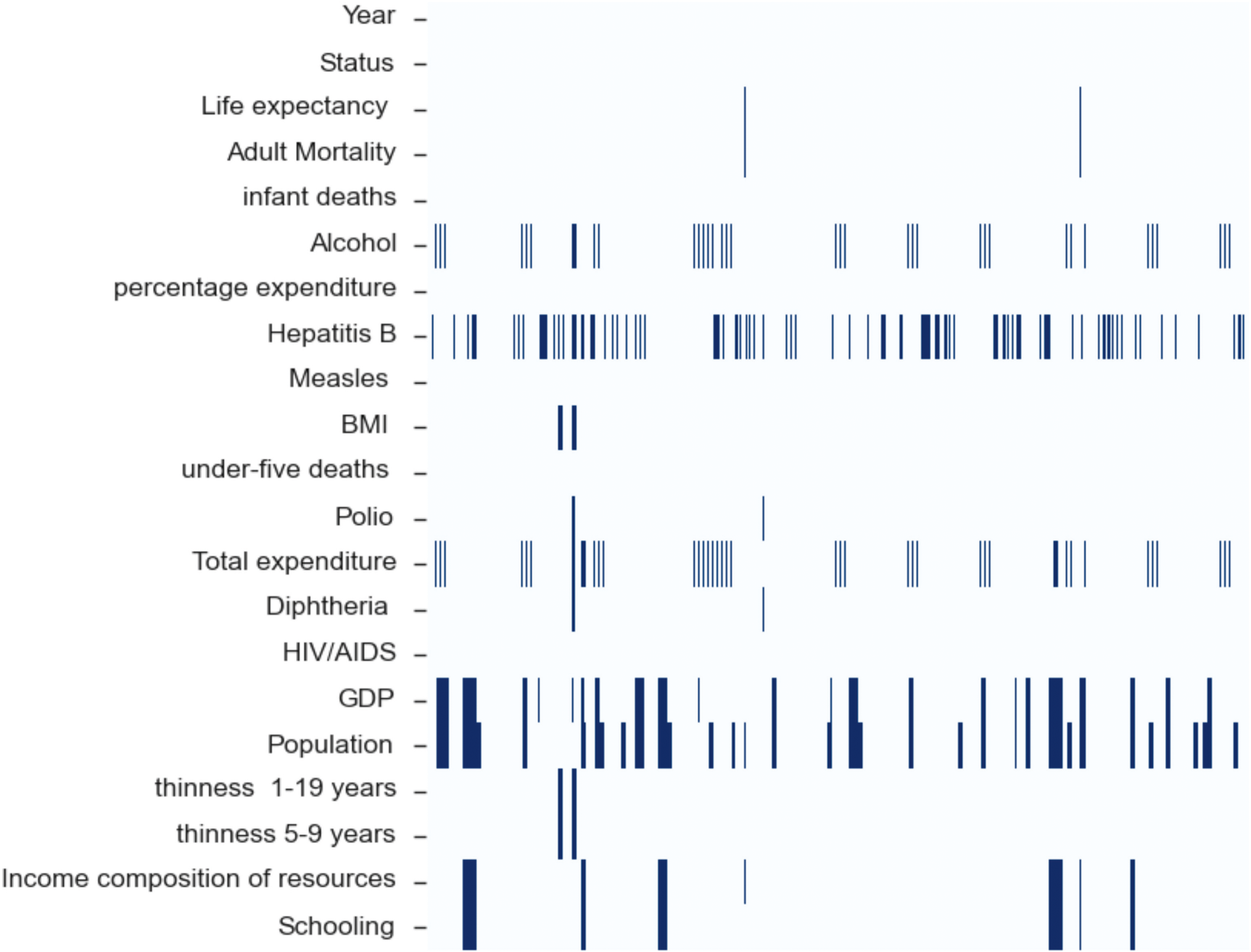
Null instances in the dataset.
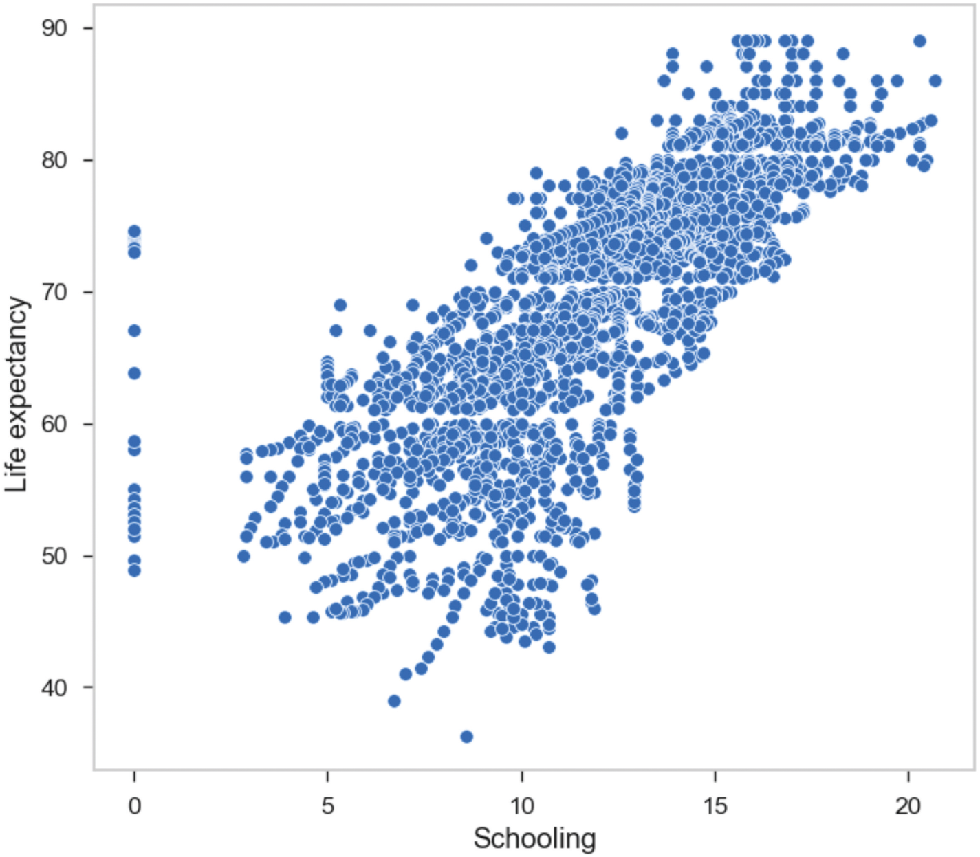
Schooling vs life expectancy.

HIV/AIDS vs life expectancy.
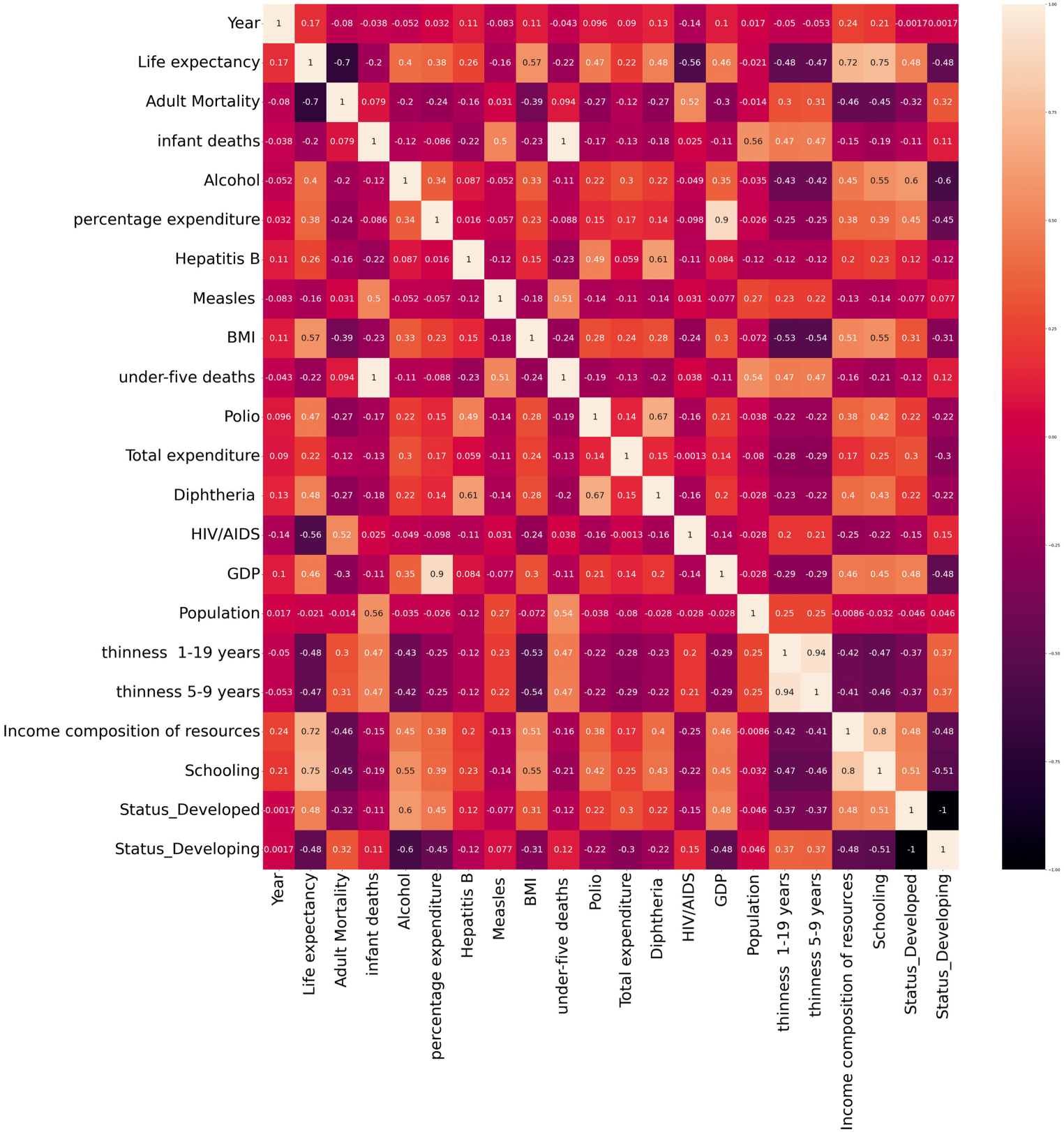
Correlation matrix.
Surrogate trees is a tree-based imputation technique that supports tree-based algorithms. It focuses on the model instance’s struggling nodes for improving overall predictions. It is used when the standard model struggles to produce accurate results, so combining the surrogate and main trees may result in an even better result. In this study, we have used the IterativeImputer class from sklearn, which acts as an imputer for multivariate datasets and considers each feature while performing the imputation.
Ridge regression
It is a statistical technique to estimate unknown parameters in a linear regression model. It is better than linear regression as it penalizes more significant coefficients that encourage the model to use hold into account for weaker features. Its optimization algorithm tries to minimize the combined loss function, resulting in a more stable and improved solution in noisy conditions in a dataset.
Multilayer perceptron regressor
An MLP regressor is an artificial neural network used to perform regression. It consists of multiple layers of neurons, which are used to predict continuous numerical values. The MLP regressor has an input layer, an output layer, and one or more intermediate hidden layers.
The data used in the analysis were obtained from the World Health Organization and sourced from Kaggle [30]. The data consisted of 193 countries with various parameters that could be used to describe life expectancy. The dataset consists of 2937 records across 22 parameters. The dataset was divided into 80% training and 20% testing based on randomization techniques. This was performed to prevent bias while selecting the data for the training and testing sets. The study was performed using Python version 3.11.2 to perform all analyses, calculations, and predictions.
Before training the regression models on the dataset, the NULL values were replaced with four different values to determine which value is best suited for each regression model and how they behave while replacing the NULL value with various values. The values used to replace the NULL values were as follows:
Mean Median Mode Interpolation Value
The fifth pre-processing technique that we used was to drop the records containing NULL values and train the regression model without them.
For data-handling operations we used the Pandas library. It provides data structure called dataframe, which holds the data in an array that is essentially a NumPy array. NumPy is another important library used to perform mathematical operations on complex structures such as arrays and matrices. The combination of NumPy and Pandas helped us clean the data and perform several operations for proper structuring before providing it to the regression model.
For visualization purposes, Matplotlib and Seaborn were used. Matplotlib is a visualization library that is typically used to plot two-dimensional graphs and visualize data. Seaborn, which is based on Matplotlib and integrates well with the dataframe, was used to create multidimensional visualizations.
In the initial phase, we applied the pre-processing. To do so, we determined the instances of NULL data in the dataset, as suggested by the diagram shown in Fig. 1.
An experimental exploratory analysis was performed to ensure that the data had parameters that were correlated with life expectancy to some extent. To do so, we plotted scatterplots of several parameters with respect to the life expectancy.
A linear pattern was observed in some scatterplots, suggesting some correlation between the parameters. The dependent variable was placed on the y-axis and the independent variables were placed on the x-axis while plotting the scatterplot. Figure 2 suggests a strong positive correlation between schooling and life expectancy.
It is clear that, as the schooling of children increases, their life expectancy also increases. Another scatter plot was plotted to assess whether HIV/AIDS affected life expectancy, or not and is shown in Fig. 3. It is clear that countries with high HIV/AIDS cases tend to have lower life expectancies than countries with a relatively lower count of HIV/AIDS. With the help of these scatterplots, it is clear that both socioeconomic and health-related factors can affect life expectancy. This analysis also confirms the presence of correlation in our dataset. Thus, to assess the correlation for all parameters available in the dataset, we visualized a correlation matrix, which is shown in Fig. 4.
The dataset consisted of a categorical variable, that is, the development status of a country. It states whether the country is already developed represented by the value ‘Developed’ or is in a state of developing, represented by the value ‘Developing’. This parameter also has to be fitted into the regression models, but to make the models consider them, we have to make these string values machine-understandable.
To solve this problem, we used one hot encoding. This technique uses numerical values to represent the categorical data [31,32,33]. This proves to be of great help because most regression models require numeric input. To apply one hot encoding to our dataset, we used the ‘get_dummies’ method from the Pandas library.
To begin with our comparative analysis, we must first split the data into X and Y parts in order to establish a relationship between them. The X-axis contains all parameters except life expectancy. In contrast, the Y-axis contains only the life expectancy. The dataset was then divided into two parts for training and testing. To achieve this, we used the ‘train_test_split’ method from the Pandas library, passing the values of the X and Y data and setting the ‘test_size’ parameter to 0.2, meaning that 20% of the dataset will be allocated for testing and the remaining 80% for training the model.
The models were trained and their results were noted in a tabular format. The following performance matrices were used are as follows:
R2 Score Adjusted R2 Score Mean Absolute Error Mean Squared Error Root Mean Squared Error
All of the above-mentioned matrices were noted for comparison. No single metric perfectly depicts the performance of the model.
The Mean Absolute Error shown in Eq. (1) is calculated by adding all the absolute differences between the actual and predicted outputs and dividing this value by the total number of observations.

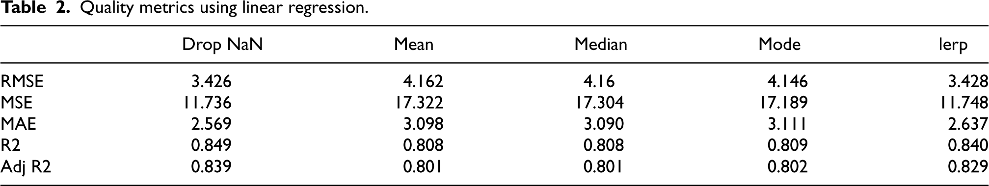
Quality metrics using linear regression.
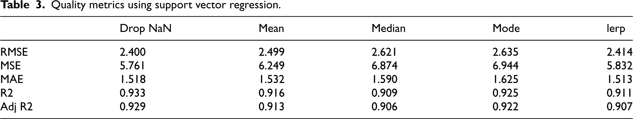
Quality metrics using support vector regression.
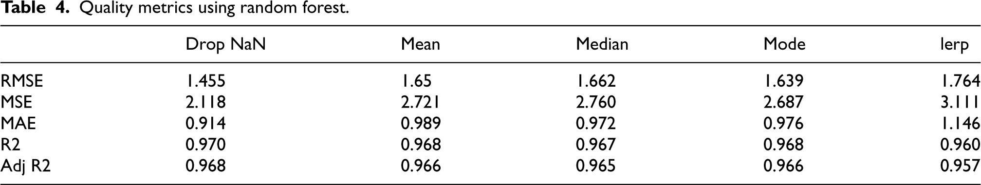
Quality metrics using random forest.
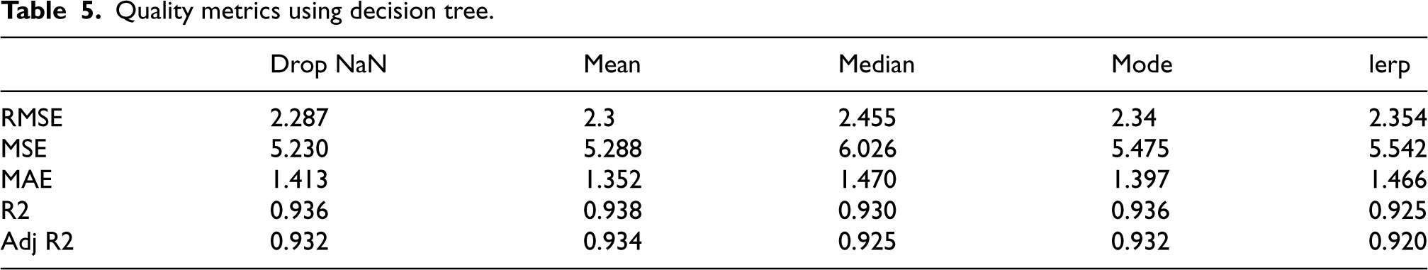
Quality metrics using decision tree.
Quality metrics using polynomial regression.

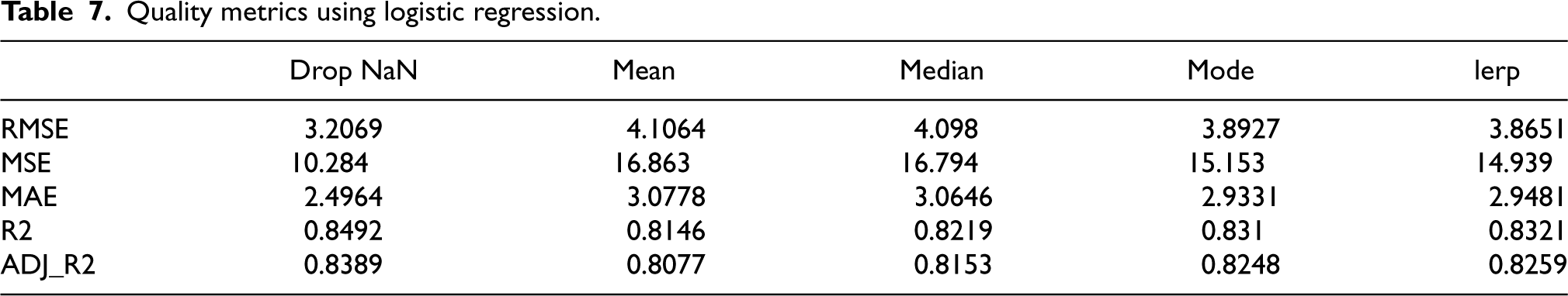
Quality metrics using logistic regression.
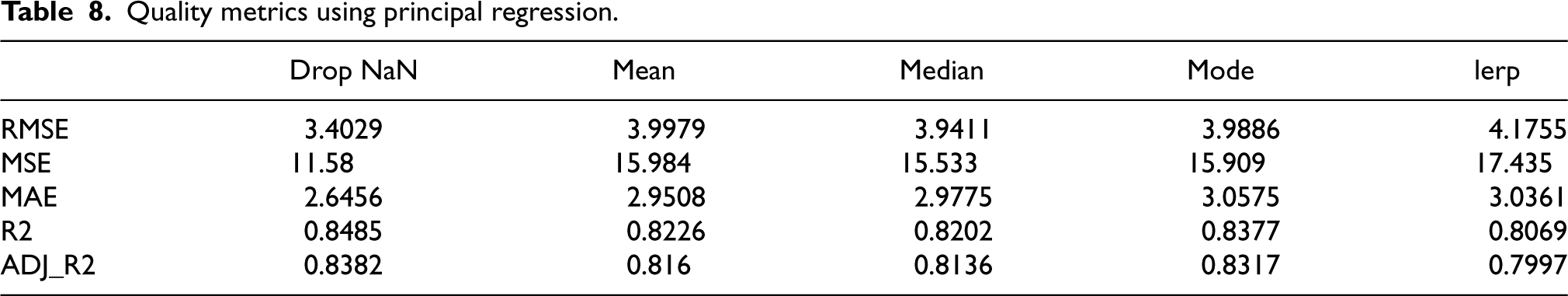
Quality metrics using principal regression.
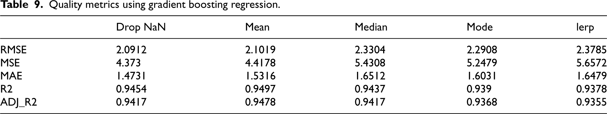
Quality metrics using gradient boosting regression.
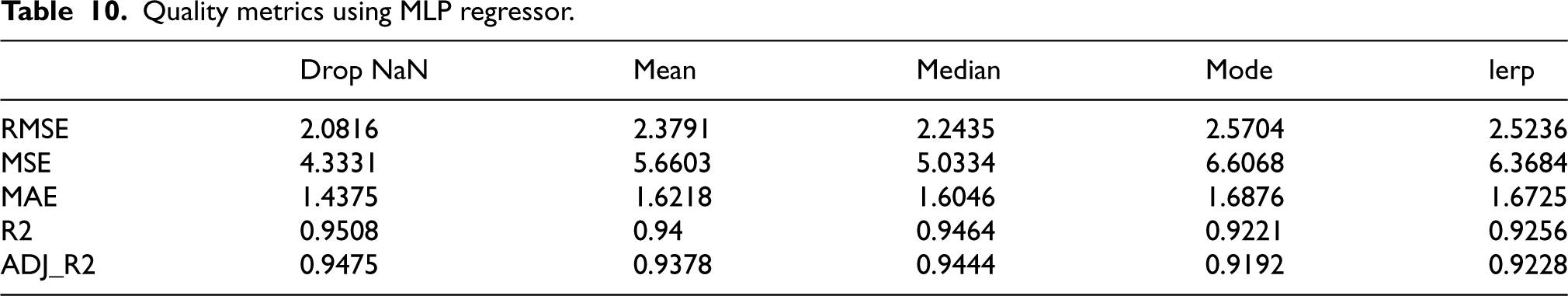
Quality metrics using MLP regressor.
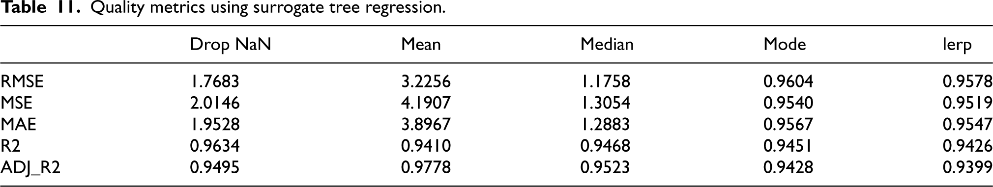
Quality metrics using surrogate tree regression.
Quality metrics using ridge regression.

The Mean Squared Error shown in Eq. (2) is calculated in a similar fashion as MAE, but before adding each absolute difference, it is squared and then divided by total observations.
The Root Mean Squared Error given in Eq. (3) can be derived simply by taking the square root of the MSE.
Root mean squared error.
Mean squared error.
Mean absolute error.
R2 score.
Adjusted R2 score.
The R2 score given in Eq. (4) is a performance metric calculated using the square sum error of the regression line and the square sum error of the mean line.

where,
SSR = Square sum error of regression line SSM = Square sum error of mean line
The Adjusted R2 score as given in Eq. (5) was calculated using the R2 score, total sample size (T), and number of independent variables (N).

The proposed algorithm performs a comparative approach of nine regression methods: Linear Regression, Support Vector Regression, Random Forest, Decision Tree, Polynomial, Logistic, Principal, Gradient Boosting, and MLP regression, which performs simulations on five different pre-processing techniques that lead to 40 different combinations of results.
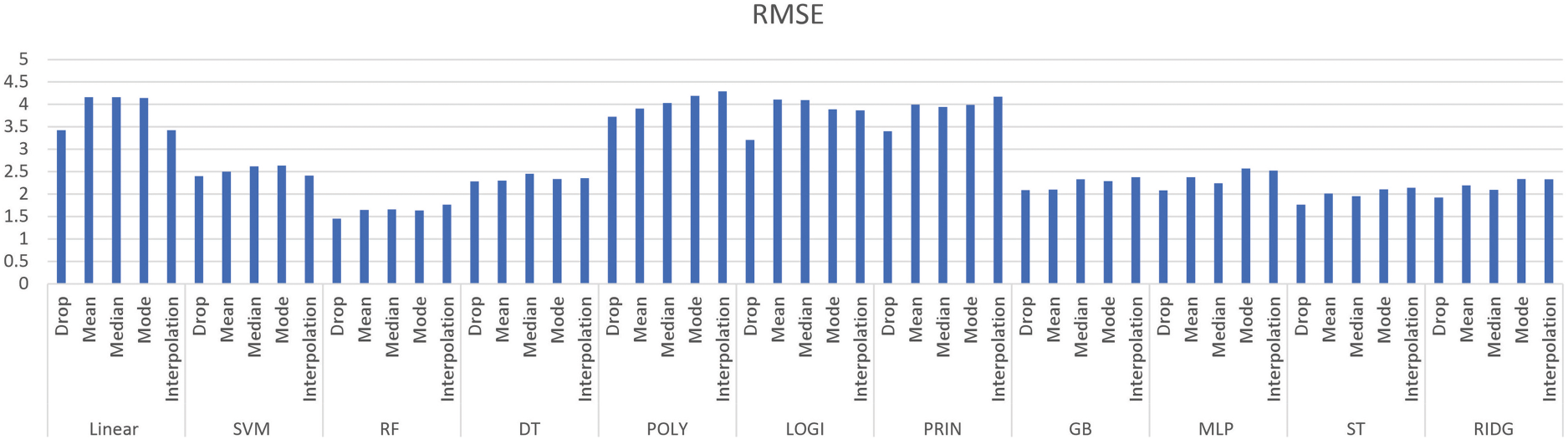
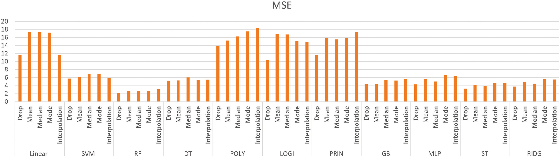
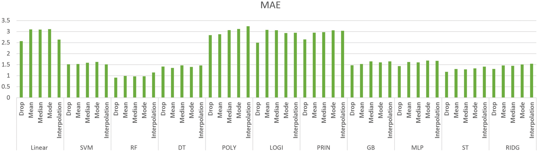
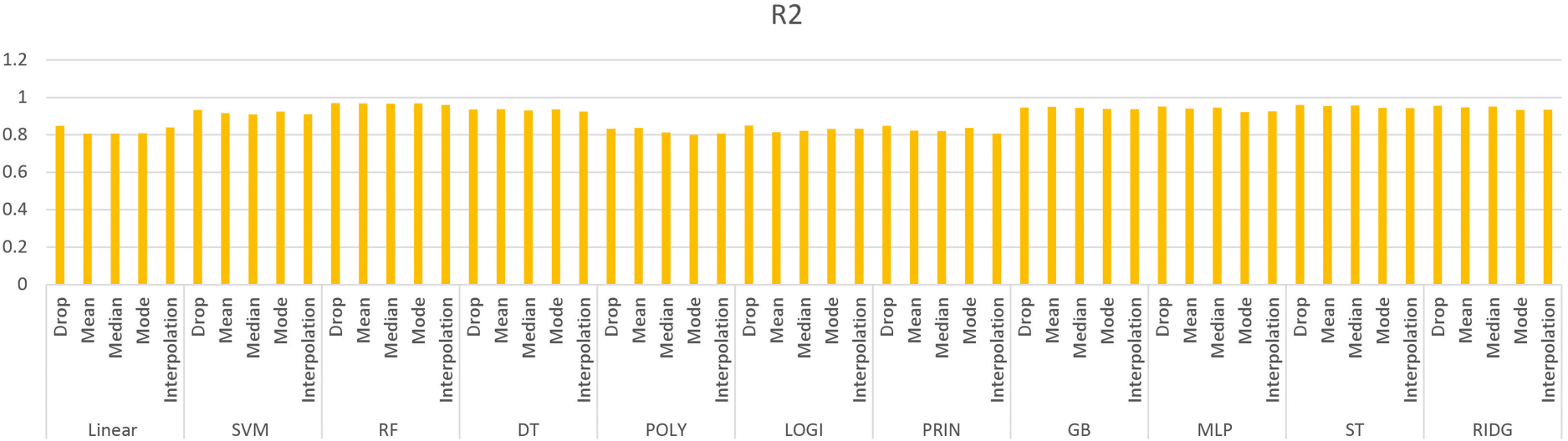
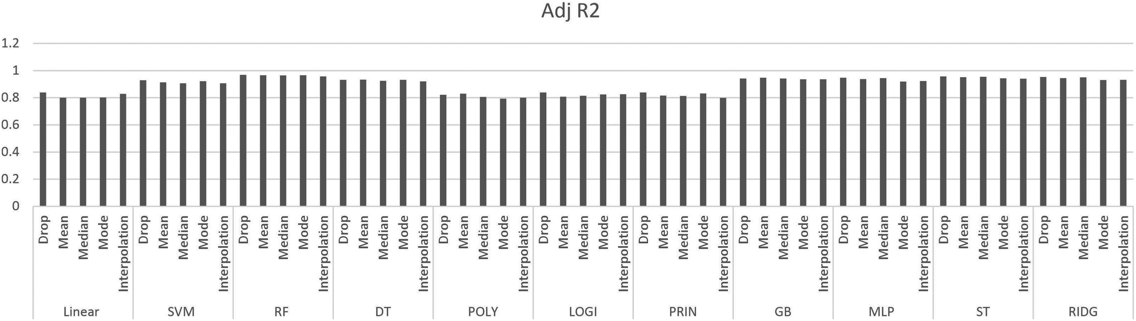
The results obtained using the eleven regression methods on five different quality parameters are shown in Tables 2–12.
The DropNAN pre-processing, that is, dropping the NULL values produced the best result as it preserves the behavior of the dataset the best. As the linear regression establishes a relation between the data points by forming a line, while replacing the NULL values with interpolation values, the missing value is filled with the midpoint of the slope, the interpolation values help boost the values for linear regression, as they help to continue the linear trend of the linear regression model.
Tree-based models, such as random forest and decision tree regressions, use mean values to make predictions, replacing the NULL values with mean values helps in continuing that prediction and prevents the formation of bias that could have been done by performing some other imputation.
Furthermore, to classify the quality parameters using the nine different regression methods, all the quality parameters were plotted as shown in Figs 5 to 9.
Conclusion and future scope
We successfully implemented all decided regression models and applied pre-processing techniques. We also tracked various performance metrics to understand the behavior of the model with different imputations.
Other imputations, such as the end-of-tail imputation, can be used with the models to obtain better results. Moreover, the method of splitting data between training and testing can be further optimized, as every time the method is called, the splitting is randomized resulting in a variance of 1–2% in every iteration of calculating the results. If this situation can be improved to obtain the same randomized training and testing values, the problem can be eliminated. In the future, more parameters related to life expectancy will be considered, along with more regression and classification techniques, to analyze life expectancy better. The current study is limited to 22 factors and 11 imputation techniques; in the future, more than 22 factors affecting life expectancy will be considered for a more concrete analysis.