An efficient feature selection technique for clustering based on a new measure of feature importance

Abstract

Feature elimination happens because either the features are irrelevant or they are redundant. The major challenge with feature selection for clustering is that relevance of a feature is not well defined. In this paper, an attempt to address this gap is made. Feature relevance is firstly defined in terms of Variability Score (VS_i), a novel score which measures a feature’s contribution to the overall variability of the dataset. Secondly, feature relevance is evaluated using entropy. VS_i is a multivariate measure of feature relevance, where as entropy is univariate. Both of them have been used in a greedy forward search to select optimal feature subset (FSELCET –VS, FSELECT –EN). Redundancy is handled using Pearson’s correlation coefficient. Dataset characteristics also influence result. Therefore it is recommended to apply both and adopt the best for that particular dataset. Extensive empirical study over thirty publicly available datasets show that the proposed method produces better performance compared to a few state of the art methods. The average feature reduction produced is 44%. No statistically significant reduction in performance (t = –0.35, p = 0.73) when compared with all features was observed. Moreover, the proposed method is shown to be relatively computationally inexpensive as well.

Keywords

Feature selection correlation entropy principal components analysis greedy forward

1 Introduction

Feature selection is one of the most important preprocessing steps in data mining and knowledge engineering. The basic objective of feature selection is to remove irrelevant and redundant features. Let ‘S’ be the set of ‘n’ features given as (f₁, f₂, …… …… , f_n), ‘b’ be the number of features to be selected (b < n), let ‘B’ (B₁, B₂, …… …… , B_nb) denote the set of all possible subsets with ‘b’ features, from the set of ‘n’ features and let nb = C (n, b) represent the cardinality of “B”. Therefore, the problem of feature selection can be stated as finding B₀ such that J (B₀) ≥ J (B_i) ∀ B_i ∈ B. This definition assumes that the number of features to be selected is known. ‘J’ may be any evaluation measure of feature subset quality. Feature selection is also known as variable selection, attribute selection or variable subset selection.

Feature selection offers the following few benefits [1 –3]

(i) Better model understandability and improved visualization

Visualization is meaningful when there are two or three features. In case of more number of features, combination of two or three features from the available features may be used for visualization. With reduced feature subset, number of such combinations reduces significantly. Also with lower number of features, the comprehensibility of the model increases.

(ii) Generalization of the model and reduced over fitting

With removal of redundant, irrelevant and noisy features, the model become generalized and over fitting is reduced. Usually this results in better performance of the model.

(iii) Efficiency in terms of time and space complexity

Both training and execution time is improved with the reduced number of features. Understandably, the data collection effort and data storage cost are also reduced.

Because of the above mentioned merits, feature selection has many applications in medical science [5], banking and finance [6], power sector [7], software engineering [8], spectroscopy [9], hypertension diagnosis [10] etc. In this context, it is worth mentioning that dimensionality reduction (Principal Component Analysis, Singular Value Decomposition, and Factor Analysis) is an alternative way of reducing the size of the problem. However as observed in [2] and [4], the semantics of the features are lost when they are transformed through projections. Consequently, it becomes difficult to incorporate domain knowledge of the features while building the model. It may be noted, subspace clustering [36], is another approach of handing the problem of dimensionality reduction.

Feature selection happens by elimination of redundant and irrelevant features. The concept of relevance or importance of a feature is well defined in case of a supervised problem and is typically assessed by some measures of association between the features and the target variable. But, absence of the said target variable, in case of unsupervised tasks, makes the feature selection process much more complex, and hence an open problem [31].

In this paper, a measure named as variability score (VS_i) for feature relevance has been proposed based on variability of the overall dataset measured in terms of the eigen values and eigen vectors. VS_i has been used in a greedy forward search (FSELECT-VS) setting to produce an optimal feature subset. VS_i is a multivariate measure as the relevance of a feature increases with its’ ability to explain the overall variability of the dataset. Recent researches [34, 35] emphasize the role of dataset characteristics in choosing a feature selection method. Therefore to make the proposed approach more generic the entropy of the feature which is a univariate measure is also used in a greedy forward search setup (FSELECT-EN), and finally it is recommended to apply both of them and select the method which produces better result for that particular dataset. Inter feature correlation has been considered to restrict inclusion of redundant features in both the approaches.

The organization of the paper is as follows: In Section II, a brief outline of feature selection methods is provided with a short review on feature selection methods for clustering. The proposed feature importance score named as variability score, and its empirical properties has been proposed and discussed in Section III. The greedy forward search algorithms using variability score and entropy have been explained in Section IV. Section V, describes materials and methods for the experimental setup. Section VI presents the results and discussions of the experiments. Section VII, summarizes the paper with concluding remarks and future scope of work.

2 Feature selection

Feature selection is a widely researched area. There are numerous proposals of feature selection methods in last three decades. A feature selection method can be categorized by answering the following questions. a) What approach is being used? b) Whether the method is for a supervised task (Classification) or an unsupervised task (Clustering)? c) How the feature subset reduction is achieved and d) what kind of output the feature selection method produces?

2.1 Approach

As noted in [2–4 , 9] there are four standard approaches or core philosophies of building a feature selection approach, which may be described as follows:

Filter: This is the most generic of all the approaches and it is algorithm agnostic. It usually employs measures like correlation coefficient, entropy, mutual information, Fisher score, etc., which analyze general characteristic of the data to select an optimal feature set. This is much simpler and faster to build compared to embedded, wrapper or hybrid approach and as a result, this method is more popular to both academicians and industry practitioners. However, it is to be noted, that wrapper and embedded methods often outperform filter methods in real data scenarios [12]. Some of the filter methods for feature selection in clustering are laplacian score [11] and SPEC [30].

Embedded: In this type of approach, feature selection is included as a component of the objective function of the algorithm itself. Examples of such approaches are decision tree, LASSO, LARS, 1-norm support vector etc.

Wrapper: In this method, the wrapper is built considering the data mining algorithm as a black box. All combinations of the feature subsets are used and tested exhaustively on the target data mining algorithm and it typically uses a measure like classification accuracy, silhouette width etc. to select the best feature subset. Wrapper methods are computationally expensive. However, there are several heuristic and greedy strategies which can be used to prune the search space. Authors have discussed about a wrapper approach for feature selection in clustering in their work [33].

Hybrid: Hybrid approach combines the best of filter and wrapper approaches. Therefore it applies properties of data distribution (Filter) to prune the feature subset space and then use the search as in case of Wrapper to find a subset.

2.2 Supervised or unsupervised

Unsupervised tasks are undoubtedly more challenging compared to supervised tasks [13]. As a result, feature selection has also been very clearly defined for classification or supervised tasks. Feature selection generally embraces the following two principles [14].

Relevance of a Feature: If a feature is relevant, then it has a strong influence on the class separability. As previously described, this particular aspect is not well defined for clustering.

Redundancy of a Feature: A feature is redundant, if variability of the feature is explained by any other feature or combination of features.

2.3 Subset reduction technique

The basic strategy of feature selection will start with the simple assumption that the features are independent of each other. In this case, the features are ranked according to various properties of the features like correlation, fisher score, mutual information etc. (For Classification). These methods can be considered as univariate as they consider all features independently.

Alternatively, search based strategies can also be used for feature selection. An exhaustive search is computationally prohibitive. Other variants like greedy (both sequential backward or forward), simulated annealing, hill climbing etc. are used for better computational efficiency. Evolutionary algorithms like genetic algorithm (GA) have also been used to prune the search space [16, 20]. In case of filter techniques, the merit or quality of a feature subset is evaluated by measures like CFS (Correlation based feature selection) [17] or mRMR (minimum redundancy maximum relevance) [18]. A feature selection approach based on search generally has the following steps [1, 19].

Selection of initial set of features.

Generation of next set of features.

Evaluation criteria for the feature subsets (How good that particular subset is?).

Stopping Criteria.

Feature selection through clustering deserves a special mention, where each feature is represented by some of its property (mostly statistical properties or meta features) and then they are clustered. Subsequently a representative feature is selected from each of the feature clusters. Feature clustering provides a better computation complexity because clustering, is not as involved as search [20, 21]. Another alternative approach of non-search based techniques is graph based techniques, where a dense sub graph indicates group of correlated features [22].

2.4 Output

As briefly described in Section 2.3, the feature selection method will either produce a score for each feature and a ranked list, or it can also produce an optimal subset. Few of the methods may produce a number of optimal subsets with a ‘goodness of fit’ measure of feature subset quality. Whichever approach may be followed, all of them need to deal with the question of feature subset cardinality. For determining the number of features there can be several strategies. It can be selected [19], either as an absolute number, or as a fraction of total features or as a threshold value of an evaluation measure. Number of features to be selected can also be determined based on the gradient of any evaluation measure.

Important dimensions of feature selection methods as discussed above are depicted in Fig. 1.

Fig.1

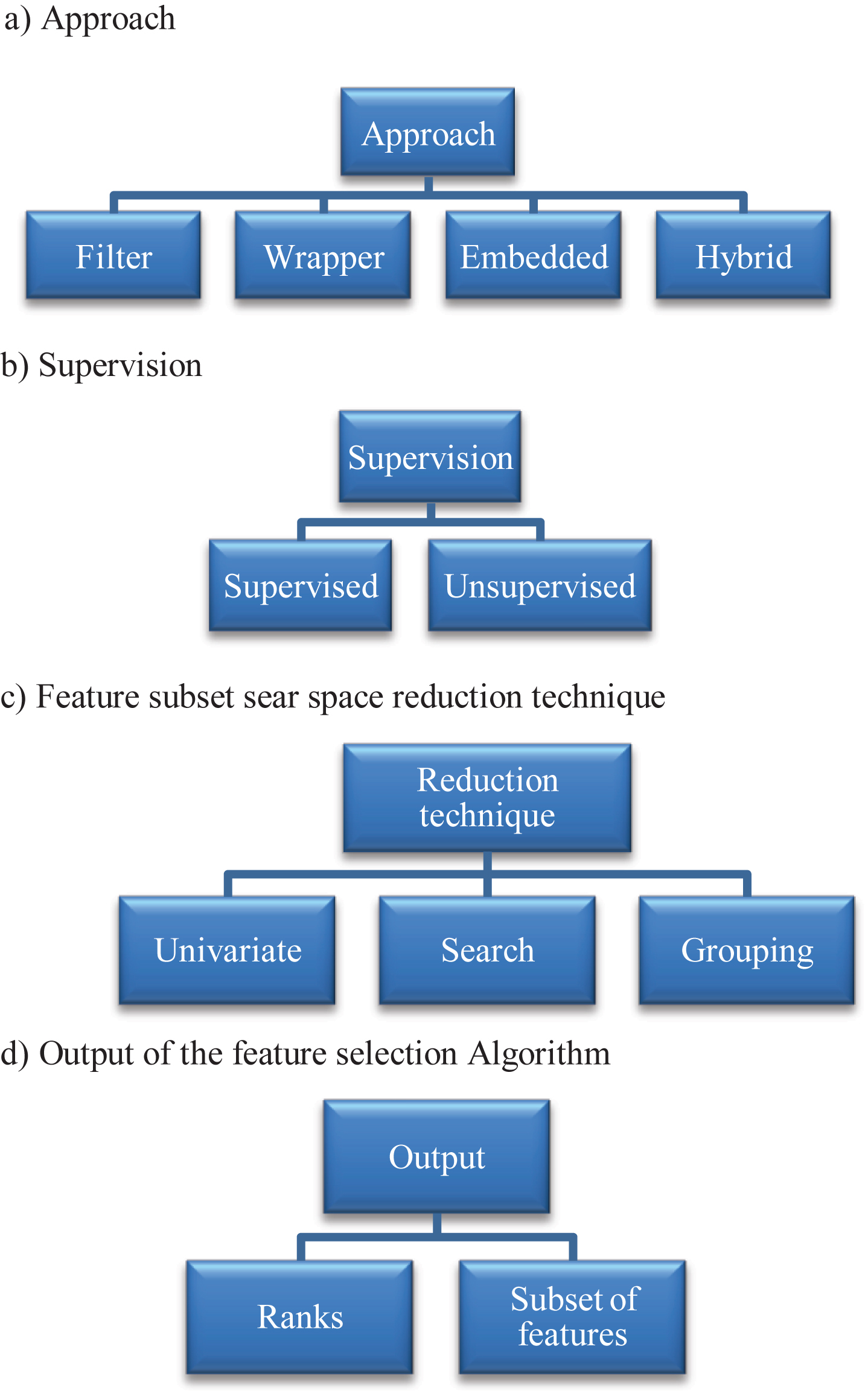
Feature selection method characteristics.

2.5 Feature selection for clustering

Clustering can be thought of as a task of dividing n-objects in k-groups such that clusters are well-formed, i.e. i) similarity between the items within a cluster (Cohesion) is very high and ii) similarity between items of different clusters is very low (Separability).

In the paper [23], a novel feature selection method named principal feature analysis (PFA) is proposed, where features are represented in terms of their contribution to the principal components and then subsequently features are clustered into ‘k’ groups. The value of ‘k’ depends on the proportion of variability that is to be retained. In a well cited work [20], the authors have defined a measure of association based on linear dependency named as Maximal Information Compression Index (λ₂) which is calculated by determining the smallest eigenvalue of Σ, where Σ denotes the correlation/ covariance matrix. The value of λ₂ is zero when the features are linearly dependent and increases as the amount of dependency decreases.

$\begin{matrix} Maximal Information Compression Index (λ_{2}) \\ = minimum (Λ_{xy}) \end{matrix}$ (1)

Finally, all features are expressed in terms of λ₂ with remaining features. Next, clustering is performed on the features to pick the best features. One representative feature from each cluster is picked subsequently. Generally this is either the cluster center or the feature closest to the cluster center. In paper [21], authors carry out feature selection for clustering in the domain of bioinformatics using feature clustering. It is also based on the same feature similarity measure as proposed in [20].

In one of the earliest works in feature selection for clustering authors have used an entropy based method [24]. The score for each feature is calculated considering pair wise similarity between each data point and hence it is computationally extensive. Finally, the above measure is used to rank the features. One other noteworthy method is based on the laplacian score [11], where features are evaluated based on locality preserving power of the features. The process involves, evaluating individual features by pairwise comparison of data values, where if the data points are not ‘close’ enough, it is marked ‘0’ or else it is marked by $e^{\frac{- (x_{i} - x_{j})^{2}}{t}}$ , where x_i and x_j are ith and jth value of the feature ‘x’ and ‘t’ is a constant. SPEC [30] is another neighborhood based method similar to [11], in fact it may be shown that, laplacian score is a special case of the same.

3 Proposed variability score

For a supervised problem, importance or relevance of a feature is easy to determine. It can be obtained by measuring the correlation coefficient, mutual information or Fisher’s Score between the feature and the target variable. However the problem is not that simple to solve in an unsupervised task. In this section, a novel measure of feature importance is proposed for unsupervised problem. It is based on principal component analysis of the dataset.

Principal component analysis (PCA) is one of the oldest and most used methods for multivariate analysis of data. In principal component analysis, given an input matrix (n x m), an output matrix(n x m) is produced by projection. The rows of the output matrix are called principal components which conform to the following rules

Variability is highest in the direction of the first principal component and then gradually it decreases with each component.

The principal components are unrelated i.e. orthogonal to each other.

The variability score is then proposed based on the following intuitions.

Higher the correlation of a feature with the principal components, higher is the capability of the feature to explain total variance of the dataset.

These correlation coefficients need to be suitably weighed and combined to arrive at a score for feature importance.

The weight should vary based on the individual principal component’s ability to explain the overall variability of the dataset.

VS_i indicates the variability score of the ith feature and VS is the set containing the VS_i of individual features given as {VS₁, VS₂, …… …… , VS_n), where n is the number of features in the dataset.

Detailed steps of computation of Variability Score (VS) are enclosed below: -

Step 1: Principal component analysis of the dataset [D] is performed (m x n matrix, m observations and n features) $Σ = A Λ A^{T}$ (2)

In the above equation, Σ denotes the correlation matrix, A is a matrix whose columns are the orthonormal eigenvectors of the matrix Σ and Λ is given as below matrix $[\begin{matrix} λ_{1} & \dots \\ ⋮ & ⋱ & ⋮ \\ \dots & λ_{n} \end{matrix}]$ where λ₁, λ₂, …… …… , λ_n are the Eigenvalues respectively, and λ₁ > λ₂ > λ₃ > …… … > λ_n.

Step 2: A subspace dimension, q is selected from n. The cardinality of q depends on the amount of variability to be retained, where variability retained is given by

$\begin{matrix} Variability Retained (VR) : \\ - (\sum_{i = 1}^{q} λ_{i} / \sum_{i = 1}^{n} λ_{i}) * 100 \end{matrix}$ (3)

Step 3: Pearson’s product moment correlation coefficient has been computed between the ‘n’ original features and ‘k’ selected principal components from previous step. It is denoted by [COR_PC] (n x k matrix, n features and k components). The absolute values of the correlation coefficients have been used.

Step 4: Variability explained (VE) is computed as a column matrix where the jth element is the variability explained by the jth eigen vector (in %) which is computed as $λ_{j} / \sum_{i = 1}^{n} λ_{i}$ .

Step 5: Variability Score [VS] is given as $[VS] = [{COR}_{PC}] [VE]$ (4)

The theoretical maximum value for VS_i is 1 when the dataset itself is univariate. Therefore, VS_i gives a positive value between 0 and 1. An empirical analysis of VS_i has been conducted over 51 publicly available datasets which consists of 3674 features.

Observations from the empirical distribution are as follows:

The values are mostly concentrated in lower range of VS_i.

The maximum values are in the range of 0.72 to 0.75.

The mean is 0.14 and median is 0.11.

It has a skewness of 1.55 and kurtosis of 2.74.

The standard deviation is 0.13.

In Fig. 2, the empirical distribution as obtained from all the features is represented using a histogram. In Fig. 3, average VS_i of each dataset is presented with a histogram.

From Fig. 2, it is evident that the values are more concentrated in the lower range of VS_i.

It can be observed from Fig. 3, that average VS_i follows the shape of a normal distribution quite closely, with the peaks between 0.2 and 0.4.

Fig.2

VS_i Empirical distribution.

Fig.3

Mean VS_i of datasets.

4 Proposed framework

Apart from VS_i, entropy has also been used to measure importance of a feature. The rationale of using both the measures is that, while VS_i focuses on overall variability of the dataset, entropy focuses on variability or information richness of individual features. Recent researches [34, 35] emphasizes on the role of dataset characteristics in choosing a feature selection method. In the proposed approach, as both the univariate and multivariate measures of feature importance is employed, it is much more generic theoretically.

Correlation coefficient has been used here for removing redundancy. Some important properties of the correlation coefficient, are that the value varies between –1 and +1, higher the absolute value, higher is the strength of the relationship between the variables. It is also symmetric, i.e., correlation coefficient between x and y and correlation coefficient between y and x is same. Correlation coefficient exhibits the property scale invariance.

As noted in [26] values of ≤ 0.35 are generally considered to represent low or weak correlation, values lying between 0.36 and 0.67 are considered to be medium or moderate correlation and values between 0.68 and 1.0 indicate strong and high correlations. Especially values ≥ 0.9 are considered as very high correlation. Some other important measures are namely Fisher’s Score, mutual information, and relief etc. However none of the other measures of dependency has such wide acceptability and clear semantics attached with it.

Next greedy forward search algorithms FSELECT-VS and FSELECT-EN have been outlined which uses VS_i and entropy respectively.

Algorithm I:

The same process is implemented with Shannon’s Entropy as well.

Shannon’s Entropy: For a finite sample, Shannon’s Entropy is taken as ∑_ip (x_i) log _b p (x_i), where x_i are the values taken by random variables, and b is the logarithmic base, taken as 2 generally. For continuous variables, suitable discretization techniques need to be applied.

FSELECT –EN, is very similar in working as that of FSELECT –FS, this uses the entropy of the features as opposed to VS_i.

Algorithm II:

Final Proposal:

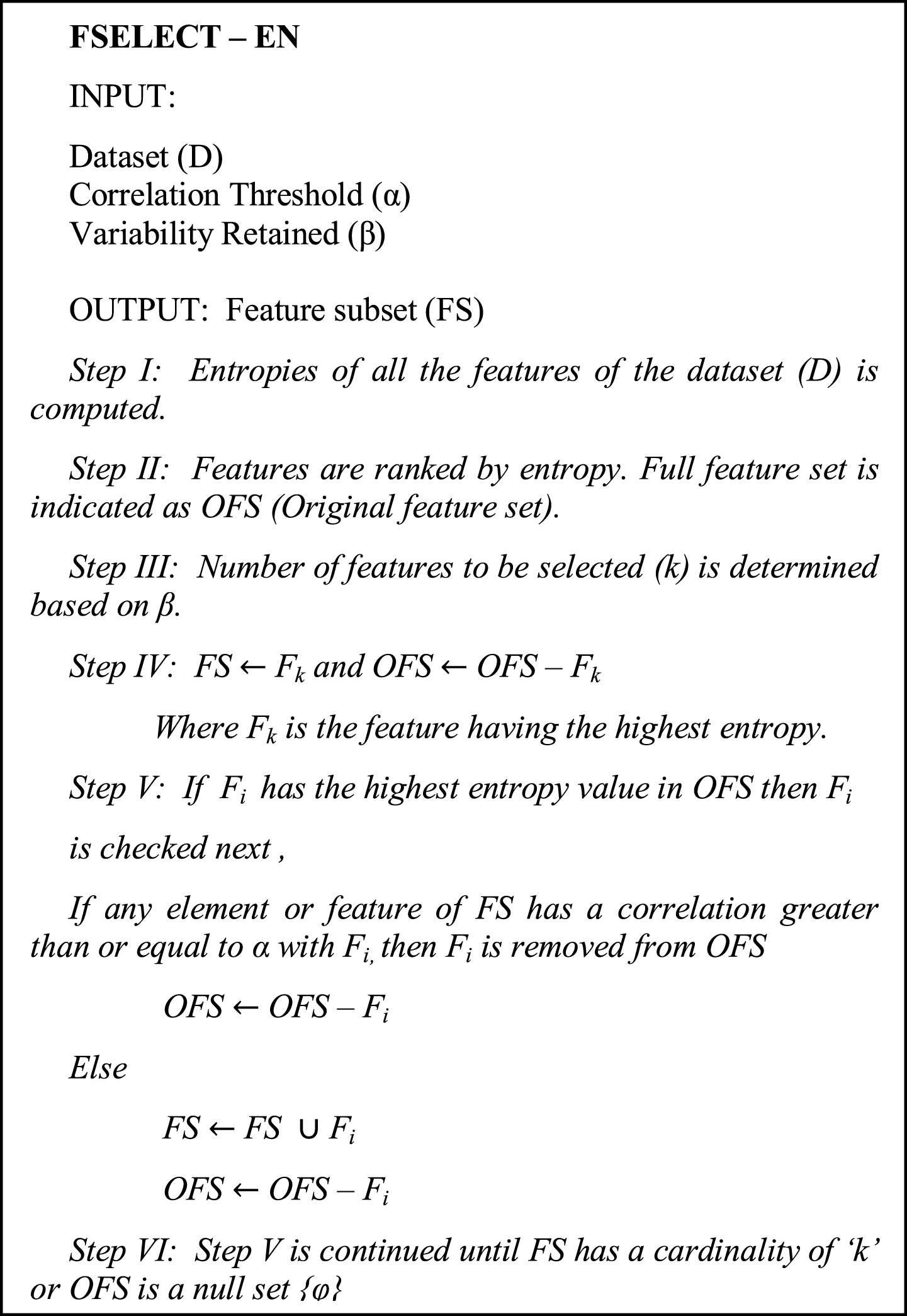
Both the above methods are computationally very inexpensive as they apply greedy forward search. VS_i has a linearity assumption. Entropy is more generic. VS_i considers overall variability of the dataset where as entropy considers individual variability of the features.

Hence it is recommended to use both the methods and use the one which is giving better result for that dataset. It is to be noted, that in individual capacity both these algorithms outperform some of the existing state of art feature selection methods. The final recommended method has been illustrated in Fig. 4.

Fig.4

Proposed Final method

5 Simulation experiment

The salient points of the experimental setup as far as materials and methods are concerned are as follows: -

30+ datasets are used from publicly available sources [27, 28]. These are basically datasets used for classification, which has been used for clustering by removing the class or target column. Actually there are many internal cluster validity measures like Silhouette Coefficient, Sum of Square Error (SSE), entropy etc. different indices give varying amounts of emphasis on cohesion and separability and hence are subjective. With labels available external cluster validity measure can be applied. The dataset details are given in Table 1.

The datasets are quite varied, with some datasets having more than 100 features (Digits, lsvt, Mdlon)

Most of the datasets have more than 2 classes making the datasets complex, with some having 10 or more classes (Segment, Yeast, Leafs, Dow, Digits etc,)

Feature selection is performed by using the two algorithms FSELECT –VS and FSELECT - EN as explained in Section IV.

The values of the parameters α (Correlation Threshold) and β (Variability Retained) have both been set at 0.9.

Both methods have been combined in the final proposed method as explained in Fig. 4.

Feature selection have also been performed using few existing methods [11 , 23] for comparison.

For determining cardinality of the optimal feature subset, β have been used. So all the methods have been compared keeping the same level of feature reduction.

The feature subsets have been compared based on the purity, which is a standard external measure of cluster validity. Purity: p_ij is defined as the probability of a member of the cluster i that belongs to the class j, and is given by m_ij/m_i, where m_ij and m_i are counts as appropriate. Now purity of a cluster i is given by $p_{i} = max_{j} p_{ij}$ . The overall purity of the dataset is given by $\sum_{i = 1}^{k} \frac{m_{i}}{m} * p_{i}$ .

The clustering algorithm used in this setup is K Means and the purity reported in the results sections is an average of 100 iterations.

The computational environment used is ‘R’ [29].

Table 1
Dataset details

Dataset Number of Number of Number of

Features Records Class

Appendicitis 7 106 2

Banknote 4 1372 2

Biodegradation 41 1055 2

Blood 4 748 2

Brest tissue 9 106 6

Bupa 6 345 2

Cleveland 13 297 5

Contra 10 1473 3

CTG 34 2126 10

Darma 34 34 6

Digits 256 1593 10

Dow 12 995 10

Ecoli 7 336 8

fertility 10 100 2

Glass 9 214 6

Heart 13 270 2

ILPD 10 579 2

Ionosphere 33 351 2

Iris 4 150 3

Leafs 11 340 30

Lsvt 310 126 2

Medlon 500 2000 2

Pima 9 768 2

Satimg 18 1166 7

Seeds 7 210 3

Segment 18 2310 10

Sonar 60 208 2

Spectf 45 267 2

Vehicle 18 846 4

Wbdc 31 569 2

Wine 13 178 3

Yeast 8 1476 10

Dataset	Number of	Number of	Number of
Appendicitis	7	106	2
Banknote	4	1372	2
Biodegradation	41	1055	2
Blood	4	748	2
Brest tissue	9	106	6
Bupa	6	345	2
Cleveland	13	297	5
Contra	10	1473	3
CTG	34	2126	10
Darma	34	34	6
Digits	256	1593	10
Dow	12	995	10
Ecoli	7	336	8
fertility	10	100	2
Glass	9	214	6
Heart	13	270	2
ILPD	10	579	2
Ionosphere	33	351	2
Iris	4	150	3
Leafs	11	340	30
Lsvt	310	126	2
Medlon	500	2000	2
Pima	9	768	2
Satimg	18	1166	7
Seeds	7	210	3
Segment	18	2310	10
Sonar	60	208	2
Spectf	45	267	2
Vehicle	18	846	4
Wbdc	31	569	2
Wine	13	178	3
Yeast	8	1476	10

6 Results and discussion

The comparisons of purity of all the methods across the datasets have been given in Table 2. At first, it is established that the feature reduction is achieved by the proposed method without any statistically significant performance degradation. Then the proposed approach is compared with other state of the art algorithms for a performance comparison.

FSELECT –VS, FSELECT –EN, PFA [23], EVA [20], Laplacian Score [11], proposed (best of FSELECT –VS, FSELECT –EN) and “All features” have been denoted as (1), (2), (3), (4), (5), (6) and (7) respectively in subsequent text.

After analysis of the results in Table 2, it can be seen

(1), (2), (3), (4), (5), (6) and (7) produce average purity of 67.3%, 66.8%, 67.4%,66.7%, 65.81%,, 68.51% and 68.79% respectively. Results produced by the proposed method (Which picks best result from FSELECT –VS and FSELECT –EN) is the closest to results obtained with all features and it achieves the same, with close to 44% (average) reduction in the feature set cardinality (Table 2 % Reduction Column).

Statistical Significance:

One of the criteria of feature reduction is that it should not result in any corresponding decrease in performance measure as compared with all features. So a pair wise t-test has been performed between results obtained by each of the 6 methods (1–6) and that obtained using all features (7).

The pair wise t-test between the results obtained from (6) and (7) is not statistically significant. (t = –0.35, p = 0.73). Same holds true for (1) and (2). It is to be noted that for (3) and (5) performance degradation because of the feature subset reduction is statistically significant. (4) Exhibits again no statistically significant performance degradation. The results of the pair wise t-tests with all features have been presented in Table 2a.

The summary results are shown in Table 3a and b. Table 3a contains average value of purity and average of the ranks. Table 3b furnishes head to head performance against the other methods. (W indicates ‘Win’, D indicates ‘Draw’ and L indicates ‘Loss’)

Average value is not a good metric to compare methods [32]. It is quite possible that for a particular dataset a method achieves superior performance by quite a margin which makes up for marginal under performance across datasets. As an example for a particular dataset CTG, (4) achieves 46% better result than (5). Therefore, a rank based comparison is done, where ranking is done based on the performance. Lower the rank of a method better is the performance. The average rank achieved by (1), (2), (3), (4), (5), (6), (7) are 3.28, 2.97, 3.66, 3.59, 4.25, 1.88 and 2.72 respectively (Table 3a).

It can be observed that, at individual level both (1) and (2) outperform (3), (4) and (5).

In (6), when the better of (1) and (2) is picked; there is significant improvement in average rank and in fact this is the only method to achieve better rank than full feature set option.

A comparison has also been made in terms of absolute number of cases where each of the methods gives equivalent or better performance as compared to (7). (1), (2), (3), (4), (5) and (6) have the count of such cases or datasets as 18, 15, 15, 14, 13 and 20 respectively.

Table 2
Clustering Accuracy across datasets and Method

Dataset % Reduction VS_i (1) Ent(2) PFA(3) EVA(4) LapScore (5) Proposed (6) Full (7)

Appendicitis 51% 84.9% 84.9% 82.1% 82.1% 82.1% 84.9% 81.0%

Banknote 25% 55.9% 55.6% 62.2% 55.5% 55.6% 55.9% 55.9%

Biodegradation 56% 66.3% 66.8% 66.3% 66.3% 73.6% 66.8% 67.0%

Blood 50% 76.2% 76.2% 76.2% 76.2% 76.2% 76.2% 76.2%

Bresttissue 55% 56.3% 51.5% 52.8% 53.3% 54.2% 56.3% 56.0%

Bupa 16% 58.0% 58.0% 58.0% 58.0% 58.0% 58.0% 58.0%

Cleveland 23% 60.4% 60.5% 59.0% 59.0% 57.4% 60.5% 60.1%

Contra 22% 42.7% 43.5% 42.7% 42.8% 42.8% 43.5% 42.7%

CTG 50% 77.5% 45.4% 96.2% 46.1% 72.4% 77.5% 95.9%

Darma 50% 87.3% 83.9% 76.4% 82.8% 82.5% 87.3% 86.7%

Digits 57% 55.0% 56.0% 62.0% 52.0% 54.5% 56.0% 59.0%

Ecoli 29% 76.0% 81.0% 78.0% 77.0% 66.0% 81.0% 82.0%

fertility 12% 88.0% 88.0% 88.0% 88.0% 88.0% 88.0% 88.0%

Glass 33% 55.0% 56.0% 53.0% 56.0% 55.8% 56.0% 55.0%

Heart 23% 82.6% 79.6% 81.5% 81.1% 80.4% 82.6% 84.4%

ILPd 30% 72.0% 72.0% 72.0% 72.0% 72.0% 72.0% 72.0%

Ionosphere 40% 70.4% 67.0% 65.2% 68.7% 64.7% 70.4% 70.7%

IRIS 50% 81.0% 84.0% 80.0% 96.0% 77.0% 84.0% 83.0%

Leafs 71% 55.6% 53.3% 47.3% 48.8% 42.1% 55.6% 54.0%

Lsvt 93% 66.7% 71.0% 66.7% 66.7% 66.7% 71.0% 66.7%

Medlon 26% 52.0% 52.0% 59.0% 58.0% 51.6% 52.0% 58.0%

Pima 11% 67.0% 67.0% 67.0% 66.0% 67.2% 67.0% 69.0%

Seeds 57% 85.0% 82.0% 85.0% 90.0% 90.0% 85.0% 92.0%

Segment 56% 67.6% 70.1% 61.1% 62.3% 56.5% 70.1% 58.8%

Sonar 63% 56.0% 54.0% 59.0% 54.0% 56.4% 56.0% 55.0%

Spectf 61% 79.4% 79.4% 79.4% 79.4% 79.4% 79.4% 79.4%

Vehicle 62% 37.0% 40.0% 37.0% 39.0% 39.4% 40.0% 38.0%

Wbdc 77% 86.0% 87.0% 89.0% 90.0% 90.0% 87.0% 91.0%

Wine 38% 89.0% 94.0% 90.0% 92.0% 88.0% 94.0% 97.0%

Yeast 12.50% 53.0% 54.0% 54.0% 54.0% 48.0% 54.0% 53.0%

Satimg 55.55% 67.8% 67.1% 57.7% 74.2% 63.9% 67.8% 58.8%

Dow 66.67% 45.9% 56.5% 54.7% 48.5% 54.0% 56.5% 57.6%

Dataset	% Reduction	VS_i (1)	Ent(2)	PFA(3)	EVA(4)	LapScore (5)	Proposed (6)	Full (7)
Appendicitis	51%	84.9%	84.9%	82.1%	82.1%	82.1%	84.9%	81.0%
Banknote	25%	55.9%	55.6%	62.2%	55.5%	55.6%	55.9%	55.9%
Biodegradation	56%	66.3%	66.8%	66.3%	66.3%	73.6%	66.8%	67.0%
Blood	50%	76.2%	76.2%	76.2%	76.2%	76.2%	76.2%	76.2%
Bresttissue	55%	56.3%	51.5%	52.8%	53.3%	54.2%	56.3%	56.0%
Bupa	16%	58.0%	58.0%	58.0%	58.0%	58.0%	58.0%	58.0%
Cleveland	23%	60.4%	60.5%	59.0%	59.0%	57.4%	60.5%	60.1%
Contra	22%	42.7%	43.5%	42.7%	42.8%	42.8%	43.5%	42.7%
CTG	50%	77.5%	45.4%	96.2%	46.1%	72.4%	77.5%	95.9%
Darma	50%	87.3%	83.9%	76.4%	82.8%	82.5%	87.3%	86.7%
Digits	57%	55.0%	56.0%	62.0%	52.0%	54.5%	56.0%	59.0%
Ecoli	29%	76.0%	81.0%	78.0%	77.0%	66.0%	81.0%	82.0%
fertility	12%	88.0%	88.0%	88.0%	88.0%	88.0%	88.0%	88.0%
Glass	33%	55.0%	56.0%	53.0%	56.0%	55.8%	56.0%	55.0%
Heart	23%	82.6%	79.6%	81.5%	81.1%	80.4%	82.6%	84.4%
ILPd	30%	72.0%	72.0%	72.0%	72.0%	72.0%	72.0%	72.0%
Ionosphere	40%	70.4%	67.0%	65.2%	68.7%	64.7%	70.4%	70.7%
IRIS	50%	81.0%	84.0%	80.0%	96.0%	77.0%	84.0%	83.0%
Leafs	71%	55.6%	53.3%	47.3%	48.8%	42.1%	55.6%	54.0%
Lsvt	93%	66.7%	71.0%	66.7%	66.7%	66.7%	71.0%	66.7%
Medlon	26%	52.0%	52.0%	59.0%	58.0%	51.6%	52.0%	58.0%
Pima	11%	67.0%	67.0%	67.0%	66.0%	67.2%	67.0%	69.0%
Seeds	57%	85.0%	82.0%	85.0%	90.0%	90.0%	85.0%	92.0%
Segment	56%	67.6%	70.1%	61.1%	62.3%	56.5%	70.1%	58.8%
Sonar	63%	56.0%	54.0%	59.0%	54.0%	56.4%	56.0%	55.0%
Spectf	61%	79.4%	79.4%	79.4%	79.4%	79.4%	79.4%	79.4%
Vehicle	62%	37.0%	40.0%	37.0%	39.0%	39.4%	40.0%	38.0%
Wbdc	77%	86.0%	87.0%	89.0%	90.0%	90.0%	87.0%	91.0%
Wine	38%	89.0%	94.0%	90.0%	92.0%	88.0%	94.0%	97.0%
Yeast	12.50%	53.0%	54.0%	54.0%	54.0%	48.0%	54.0%	53.0%
Satimg	55.55%	67.8%	67.1%	57.7%	74.2%	63.9%	67.8%	58.8%
Dow	66.67%	45.9%	56.5%	54.7%	48.5%	54.0%	56.5%	57.6%

Table 2a

Result of pair wise t-tests

Methods	t-value	p-value
FSELECT –VS (1)	–1.66	0.11
FSELECT –EN (2)	–1.18	0.25
PFA (3)	–2.24	0.03
EVA (4)	–1.18	0.25
LapScore (5)	–2.9	0.006
Proposed (6)	–0.35	0.73

Table 3a

Overall comparison between the methods

Methods	Average Purity	Average Rank
FSELECT –VS (1)	67.30%	3.28
FSELECT –EN (2)	66.80%	2.97
PFA (3)	67.40%	3.66
EVA (4)	66.70%	3.59
LapScore (5)	65.81%	4.25
Proposed (6)	68.51%	1.88
Full (7)	68.79%	2.72

Table 3b

Comparing the win loss of the methods

Methods	FSELECT –EN (2)	PFA (3)	EVA (4)	LapScore (5)	Proposed (6)	Full (7)
FSELECT –VS (1)	W (10), D (8), L (14)	W (11), D (11), L (10)	W (13), D (7), L (12)	W (17), D (6), L (9)	W (0), D (18), L (14)	W (8), D (10), L (14)
FSELECT –EN (2)		W (16), D (7), L (9)	W (15), D (8), L (9)	W (18), D (6), L (8)	W (0), D (22), L (10)	W (10), D (5), L (17)
PFA (3)			W (9), D (10), L (13)	W (15), D (7), L (10)	W (6), D (8), L (18)	W (8), D (7), L (17)
EVA (4)				W (13), D (8), L (11)	W (5), D (7), L (20)	W (8), D (7), L (17)
LapScore (5)					W (5), D (5), L (22)	W (7), D (6), L (19)
Proposed (6)						W (14), D (6), L (12)

Table 4

Comparison of execution times (in seconds)

Dataset	FSELECT - VS (1)	FSELECT - EN (2)	PFA (3)	EVA (4)	Lscore (5)
Biodegradation	0.02	0.02	0.6	1.86	197.98
Dow	0.005	0.005	0.12	0.18	85.29
Ionosphere	0.02	0.04	1.55	3.09	5.11
lsvt	0.047	0.035	9.6	23.1	4.71
Medlon	6.93	1.69	406.2	852.6	17003
Satimg	0.18	0.41	0.008	0.008	109.2
Segment	0.02	0.02	0.18	0.51	1193.2
Digits	0.66	0.66	18.47	72.23	3822.38

It can also be seen FSELECT –VS enjoys most number of no loss situation cases and a better average purity, FSELECT - EN on the other hand achieves the best rank across datasets. Hence the combined scheme (6), to pick the best from these two has been proposed. As previously discussed, it can be seen from Table 3a, that by both average rank and average purity (6) is the best method.

In terms of computational complexity, a greedy search is quite efficient as compared with other methods; a comparison of execution time is presented in Table 4. The comparison has been limited to datasets having relatively larger number of rows or columns. The execution time has been measured in seconds.

It can be observed that, (1) and (2) take far lesser time as compared to (3), (4) and (5). The neighborhood based method (5) is most expensive, followed by clustering based methods (3) and (4). The proposed algorithms (1) and (2) demonstrate most efficient execution in terms of running time. Our finally proposed method (6) picks the better of (1) and (2). Therefore, it naturally possesses the same executionefficiency.

7 Conclusion and future work

Relevance of a feature for unsupervised problems is not adequately defined. To address this gap, in this paper, a novel variability based score named as VS_i has been proposed to measure feature importance for unsupervised problems. The above measure has been used for selecting feature subsets (FSELECT –VS) in a greedy forward search method. Correlation coefficient has been used to filter out redundant features. It can be seen, FSELECT –VS gives the best performance among the methods in terms of count of datasets in which it gives better or equivalent features as compared to using all features. Similar setting has also been used where feature importance has been measured using Shannon’s Entropy (FSELECT –EN). In the proposed framework, it is recommended to apply both the methods and select the one, which is better performing for that particular dataset.

Comparison with all featuresand the proposed method

On an average a 44% reduction in feature subset is achieved.

It is also demonstrated that, the reduction is achieved without any statistically significant decrease in performance (t = –0.35, p = 0.73).

In 19 out of 32 datasets a better or equivalent result is obtained.

In terms of average ranks, the proposed method outperforms significantly (1.88 as opposed to 2.72).

Three widely cited techniques have been selected for comparison with the proposed method.

Comparison with other state of the art methods;

The proposed method is superior in terms of average accuracy, average rank, as well as by count of datasets in which better or equivalent results are achieved.

Most importantly, superior results are achieved with a much reduced execution time.

This procedure may be extended to other nonlinear relationships as well. Nonlinear measures of the relationship between variables, as outlined in [30] or non linear PCA can be a used to relax the linearity assumption.

References

Liu

and Yu

, Toward integrating feature selection algorithms for classification and clustering, IEEE Transactions on Knowledge and Data Engineering 17(4) (2005).

Guyon

and Elisseeff

, An introduction to variable and feature selection, Journal of Machine Learning Research (2003), 1157–1182.

Liu

, Motoda

, Setiono

and Zhao

, Feature selection: An ever evolving frontier in data mining, In Proc The Fourth Workshop on Feature Selection in Data Mining 4 (2010), 4–13.

Saeys

, Inza

and Larranãga

, A review of feature selection techniques in bioinformatics, Bioinformatics 23(19) (2007), 2507–2517.

Revett

, Gorunescu

and Salem

, Feature selection in Parkinson’s disease: A rough sets approach, In Computer Science and Information Technology IMCSIT’09 International Multiconference on, IEEE, 2009, pp. 425–428.

Huang

C.L.

and Tsai

C.Y.

, A hybrid SOFM-SVR with a filter-based feature selection for stock market forecasting, Expert Systems with Applications (2009), 1529–1539.

Erişti

, Uçar

and Demir

, Wavelet-based feature extraction and selection for classification of power system disturbances using support vector machines, Electric Power Systems Research 80(7) (2010), 743–752.

Oliveira

A.L.

, Braga

P.L.

, Lima

R.M.

and Cornélio

M.L.

, GA-based method for feature selection and parameters optimization for machine learning regression applied to software effort estimation, Information and Software Technology 52(11) (2011), 1155–1166.

Balabin , Roman

and Smirnov

S.V

, Variable selection in near-infrared spectroscopy: Benchmarking of feature selection methods on biodiesel data, Analytica Chimica Acta 692 (2011), 63–72.

10.

Chao-Ton

and Yang

C.-H.

, Feature selection for the SVM: An application to hypertension diagnosis, Expert Systems with Applications 34(1) (2008), 754–763.

11.

Xiaofei

, Cai

and Niyogi

, Laplacian score for feature selection, In Advances in Neural Information Processing Systems 50 (2005), 7–514.

12.

Salem

, Tang

and Liu

, Feature selection for clustering: A review, Data Clustering: Algorithms and Applications 29 (2013).

13.

Jain

A.K.

, Data clustering: 50 years beyond K-means, Pattern Recognition Letters 31(8) (2010), 651–666.

14.

Lei

, Liu

, Efficient feature selection via analysis of relevance and redundancy, The Journal of Machine Learning Research (2005), 1205–1224.

15.

Leardi , Riccardo

, Boggia and Terrile

, Genetic algorithms as a strategy for feature selection, Journal of Chemometrics 6(5) (1992), 267–281.

16.

Goswami

, Saha

, Chakravarty

, Chakrabarti

and Chakrabarty

, A new evaluation measure for feature subset selection with genetic algorithm, International Journal of Intelligent Systems and Applications 7(10) (2015), 28–36.

17.

Hall and Mark

, Correlation-based feature selection for machine learning. Diss, The University of Waikato, 1999.

18.

Hanchuan

, Long

and Ding

, Feature selection based on mutual information criteria of max-dependency, max-relevance, and min-redundancy, IEEE Transactions on Pattern Analysis and Machine Intelligence 27(8) (2005), 1226–1238.

19.

Antonio

A.-A.

, Aznarte

J.L.

and Benítez

J.M.

, Empirical study of feature selection methods based on individual feature evaluation for classification problems, Expert Systems with Applications 38(7) (2011), 8170–8177.

20.

Pabitra

, Murthy

C.A.

and Pal

S.K.

, Unsupervised feature selection using feature similarity, IEEE Transactions on Pattern Analysis and Machine Intelligence 24(3) (2002), 301–312.

21.

Guangrong

, et al., A novel unsupervised feature selection method for bioinformatics data sets through feature clustering, Granular Computing, 2008 GrC 2008 IEEE International Conference on IEEE 2008.

22.

Sanghamitra

, Bhadra

, Mitra

and Maulik

, Integration of dense subgraph finding with feature clustering for unsupervised feature selection, Pattern Recognition Letters 40 (2014), 104–112.

23.

Yijuan

, et al., Feature selection using principal feature analysis, Proceedings of the 15th International Conference on Multimedia ACM, 2007.

24.

Luis

, Feature selection as a preprocessing step for hierarchical clustering, ICML 99 (1999).

25.

Zheng

and Liu

, Spectral feature selection for supervised and unsupervised learning, In Proceedings of the 24th International Conference on Machine Learning, ACM , 2007, pp. 1151–1157.

26.

Richard

, Interpretation of the correlation coefficient: A basic review, Journal of Diagnostic Medical Sonography 6(1) (1990), 35–39.

27.

Bache

and Lichman

, UCI Machine Learning Repository [http://archive.ics.uci.edu/ml], University of California, School of Information and Computer Science, Irvine, CA, 2013. .

28.

Alcalá-Fdez

, Fernandez

, Luengo

, Derrac

, García

, Sánchez

and Herrera

, KEEL data-mining software tool: Data set repository, integration of algorithms and experimental analysis framework, Journal of Multiple-Valued Logic and Soft Computing 17(2-3) (2011), 255–287.

29.

Core Team

, R: A language and environment for statistical computing, http://www.R-project.org/, R Foundation for Statistical Computing, Vienna, Austria, ISBN 3-900051-07-0, URL, 2013.

30.

Reshef

D.N.

, Reshef

Y.A.

, Finucane

H.K.

, Grossman

S.R.

, McVean

, Turnbaugh

P.J.

, Lander

E.S.

, Mitzenmacher

and Sabeti

P.C.

, Detecting novel associations in large data sets, Science 334(6062) (2011), 1518–1524.

31.

Guyon

, Gunn

, Nikravesh

and Zadeh

L.A.

, Feature extraction: Foundations and applications. Springer, vol. 207, 2008.

32.

Janez

, Statistical comparisons of classifiers over multiple data sets, The Journal of Machine Learning Research 7 (2006), 1–30.

33.

J.G.

, Brodley

C.E.

, Feature selection for unsupervised learning, J Mach Learn Res 5 (2004), 845–889.

34.

Guangtao

, Song

, Sun

, Zhang

, Xu

and Yuming

, A feature subset selection algorithm automatic recommendation method, Journal of Artificial Intelligence Research (2013).

35.

Saptarsi

, Chakrabarti

, Chakraborty

, Analysis of correlation structure of data set for efficient pattern classification, IEEE 2nd International Conference on Cybernetics (CYBCONF),IEEE, 2015, pp. 24–29.

36.

Parsons

, Haque

and Liu

, Subspace clustering for high dimensional data: A review, ACM SIGKDD Explorations Newsletter 6(1) (2004), 90–105.