Mobile robot navigation using PSO-optimized fuzzy artificial potential field with fuzzy control

Abstract

The objective of this paper is to develop a path planning algorithm that is able to plan the trajectory of mobile robots from its start point to target point in static and dynamic unknown environments. The classical artificial potential field (APF) method is not sufficient and ineffective for that purpose since it has the problem of local minima. To enhance the performance of the classical APF algorithm and to produce a more efficient and effective path planning for mobile robots, a new method based on combination of a modified APF algorithm with fuzzy logic (i.e. FAPF) is proposed. The proposed algorithm is designed to overcome the problems of the classical APF especially the local minima and enhances the navigation in complex environments. The fuzzy logic controller (FLC) is also used for motion control of the mobile robot. The membership functions of the FLC are optimized with particle swarm optimization (PSO) algorithm for optimality. Simulation models for the proposed path planning and motion control methods are built with MATLAB. Simulation results are obtained and proved that the robot with FAPF navigates with smoother path, react much faster in static and dynamic environments, and avoid obstacles efficiently. The work is compared with other implementations that used conventional PID controllers. All the system is then implemented practically to prove the proposed algorithms and tested in complex and unknown environment.

Keywords

Path planning fuzzy logic artificial potential field fuzzy artificial potential field PSO

1 Introduction

In spite of the great advances in the field of robotics during the last decade, there are many difficulties that robots face during navigation in real environments. This is due to the fact that the real environments are complex, unknown, uncertain, and dynamic. Navigation is one of the most important and complex tasks with which the robot should move from one position to another in collision-free paths. It is necessary for the mobile robot to navigate safely across the environment. Hence, the robot should plan the path leading to the goal point. The purpose of path planning is to find a sequence of directed movements for the robot around obstacles and avoid collisions while reaching the desired destination. There are many methods and algorithms for path planning that have been developed over the past twenty years such as: A* algorithm [1], roadmap method [2], reinforcement learning [3], potential field methods [4], neural networks [5], and fuzzy logic [6]. Each method has its own force over others in certain issues. APF method is commonly used for mobile robot path planning. With this method, the mobile robot is considered to be subjected to two artificial potential forces: attractive force and repulsive force. The obstacles generate repulsive forces against the robot, which is inversely proportional to the distance between them and is pointing away from obstacles. The destination (goal) point has attractive force that attracts robot to that goal point. APF has many benefits that make it favorable in path planning such as: simple, fast reaction, high efficiency, path is generated in real-time and less computation time. However, APF suffers from problems of local minima that occur when sum of the overall forces acting on the robot is zero. In this case the robot stops and never reaches its goal. To enhance the performance of the APF and to solve the local minima problems, a fuzzy logic is combined with the APF to get a fuzzy APF (FAPF) path planning method. Another important issue that must be taken into consideration is the motion control. Motion control is a sub-field of automation, in which the position or velocity of robots are controlled by embedded controllers. It encompasses every technology related to the movement of objects driven by electrical motors (DC or servo). In this work, another FLC is used as a motion controller for the designed mobile robot. There are many advantages for FLC such as: easy to understand, based on natural language, flexible, can be adaptive, and its parameters can be optimized easily. The optimization algorithm adopted in this paper for FLC, APF, and PID parameters is the PSO. PSO is a computational method that optimizes a problem by iteratively trying to improve a candidate solution with regard to a given measure of quality. It starts with a population of candidate solutions (dubbed particles) and moving these particles around in the search-space according to simple mathematical formula over the particles position and velocity. Each particle movement is influenced by its local best known position, but it is also guided toward the best known positions in the search-space, which are updated as better positions that are found by other particles. This is expected to move the swarm toward the best solutions. PSO is metaheuristic as it makes few or no assumptions about the problem being optimized and can search very large spaces of candidatesolutions.

Simulation results for the proposed schemes needs a mathematical model for the mobile robot to test its effectiveness. The modeling of the differential drive mobile robot used in this work is based on kinematics and dynamic modeling. Kinematics model deals with the geometric relationships that govern the system motion without adopting forces. Dynamic model takes into consideration the forces and energies affecting the robot.

The resulting developed system, which is called FAPF-FC, is compared with a conventional APF-PID systems and FAPF-PID designed for the sake of comparison. The proposed algorithm is embedded as a software package in an Arduino Mega 2560 microcontroller board along with other hardware components (five IR sensors, two DC motors vehicle, two rotary encoders, motors driver, batteries) to get a practical setup of the mobile robot.

There are many publications in the field of path planning, motion control, and APF. Khatib’s presented a potential field on the configuration space with a minimum at the target point and potential hills at all obstacles [7]. Chengqing et al. introduced a navigation method, which combined virtual obstacle concept with a potential-field-based method to maneuver cylindrical mobile robots in unknown environments. The method illustrates accepted performance and ability to solve some of the local minima problem related with potential field method [8]. A potential function is proposed by Ge and Cui that takes into consideration dynamic environments that contain moving obstacles and goals. In this work positions and velocities of robots, obstacles, and goals are considered in the functions of potential field [9]. GNRON problem (goals non-reachable with obstacle nearby), which is a common drawback in potential field methods, is identified by Ge and Cui [10] and Mei Wang et al. [11]. GNRON problem was solved using their proposed potential field method. Evolutionary Artificial Potential Field (EAPF) for real-time robot path planning is proposed by Vadakkepat et al. [12]. Combination between genetic algorithm and the artificial potential field method is introduced to derive optimal potential field functions. Pradhan et al., presented a potential field navigation method optimized by simulated annealing and hybridized with neuro-fuzzy technique to improve robot navigation in cluttered environment [22]. In this paper, we present a novel method for navigation of mobile robot using an intelligent APF with intelligent motion controller in different static and dynamic unknown complex environments.

The rest of this paper is organized as follows: Section 2 presents the problem statement via representation of the APF method with its benefits and drawbacks. Section 3 presents the mathematical modelling of the mobile robot with its two models. Section 4 discusses the motion control of mobile robot. Section 5 discusses the path planning methods designed for robot moving in different environments. Section 6 outlined experimental setup and the required hardware components. Simulation and experimental results are described in Section 7 to demonstrate the effectiveness of the proposed method for moving of the robot. Section 8 presents conclusions.

2 Problem statement

To understand the idea of APF, one can imagine that all obstacles generate repulsive forces against the mobile robot that repels it away from obstacles. The target point generates attractive force to pull up the robot towards the target. The sum of these forces results in a total force with magnitude and direction.

The robot must follow that direction to avoid obstacles and moves towards target point as shown in Fig. 1. Classical APF has four common problems or cases with which the robot trapped and stopped.

Fig.1

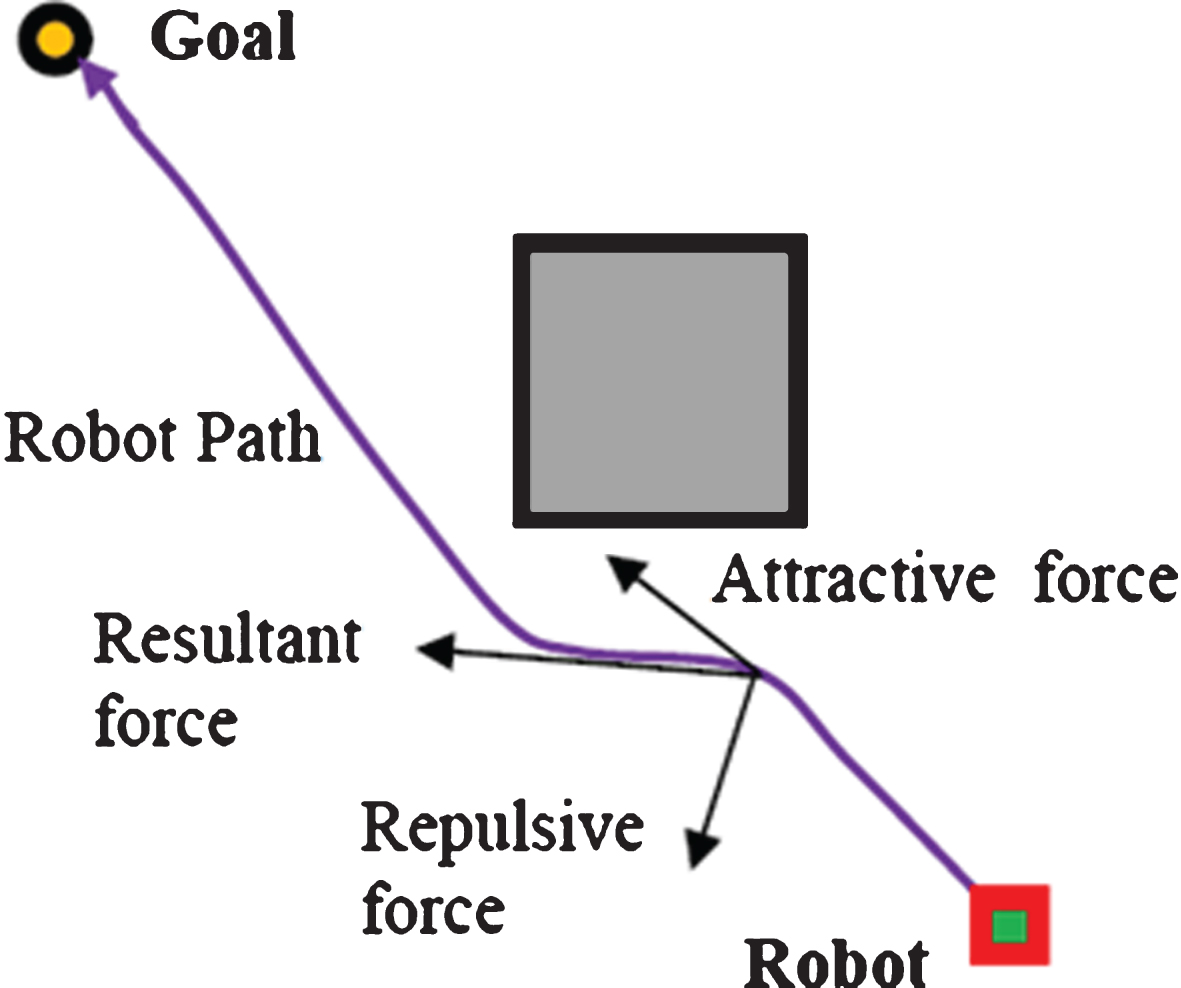
Effect of forces on the robot.

Case 1: When the robot is far away from target, the attractive force becomes large and hence the robot moves too close to the obstacles and may collide with them.

Case 2: When the robot, obstacle, and target are located on the same line with obstacle positioned in the middle of the line [13] as shown in Fig. 2a. In this case the two forces are equal in magnitude and opposite in direction leading to a zero force acting on the robot. This leads to stopping the robotnavigation.

Case 3: When the goal point is within the region of effect of an obstacle such that the repulsive force of the obstacle pushes the robot away from the goal point [14] as shown in Fig. 2b.

Case 4: When the robot encounters a complex environment that contains a complex shape obstacles e.g. a non-convex U-shaped obstacle [15] as shown in Fig. 2c. The robot is trapped inside this region.

All the aforementioned problems are solved in this paper by the proposed FAPF-FC intelligent method. This will be explained in the subsequent sections.

Fig.2

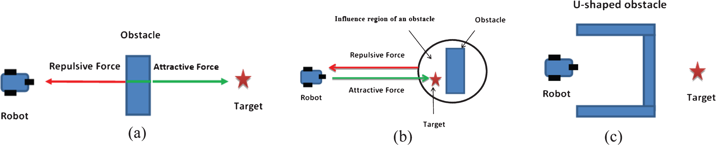
The different cases of local minima propblem of the classical APF.

2.1 Repulsive potential field function

As seen from cases 1 & 2, which occur as the robot approaches to its target, the repulsive force increases due to presence of obstacle near the target point. Therefore, the resultant force at goal point is not global minimum and that prevents the robot from reaching the target. To solve this problem, it is needed to construct a repulsive potential function that makes the target having a global minimal potential force. This can be done by introducing the distance between the mobile robot and goal into the function of repulsive force to ensure that the global minimum is at the position of the target. If the repulsive potential force becomes zero, the mobile robot will reach the target. The repulsive potential function is then given by: $\begin{matrix} \underset{rep}{U} (q) \\ = {\begin{matrix} \frac{1}{2} η {(\frac{1}{d (q, q_{obs})} - \frac{1}{d_{o}})}^{2} d (q, q_{goal})^{n}, & if \to d (q, q_{obs}) < d_{o} \\ 0, & if \to d (q, q_{obs}) > d_{o} \end{matrix} \end{matrix}$ (1)

Where d (q, q_goal) represents the distance between the robot and the goal, d (q, q_obs) represents the distance between the robot and the obstacle, n is a real number greater than 0, d_o is a positive constant representing the distance of influence of an obstacle, and η is an adjustable constant representing the proportional coefficient of the repulsive potential field function. The repulsive force is the negative gradient of repulsive potential field function. Above equation represents modified repulsive potential function to eliminate shortage in traditional function by adding d (q, q_goal), so now when the mobile robot is close to the target, the attractive potential field is reducing, the repulsive potential field is also reducing, until the mobile robot reaches the target point, then the attractive and repulsive field reduced to 0. The repulsive force can be decomposed into two types of forces:

$\begin{matrix} \underset{rep}{F} & = & - \nabla \underset{rep}{U} (q) \\ = & {\begin{matrix} \underset{rep 1}{F} + \underset{rep 2}{F}, & if \to d (q, \underset{obs}{q}) < d_{0} \\ 0, & if \to d (q, \underset{obs}{q}) > d_{0} \end{matrix} \end{matrix}$ (2)

Where F_rep1 and F_rep2 are described by: $\underset{rep 1}{F} (q) = η (\frac{1}{d (q, q_{obs})} - \frac{1}{d_{o}}) \frac{d (q, q_{goal})^{n}}{d (q - q_{obs})^{2}}$ (3) $\underset{rep 2}{F} (q) = - η \frac{n}{2} (\frac{1}{d (q, q_{obs})} - \frac{1}{d_{o}}) d (q, q_{goal})^{n - 1}$ (4)

The direction of F_rep1 points to the robot from the point, which is closest to the robot. The direction of F_rep2 points to the target from the robot.

2.2 Attractive potential field function

The value of the attractive potential field is calculated by the distance d (q, q_goal). When mobile robot is far away from goal point, the attractive force becomes large. This leads the mobile robot to move too close to the obstacles. Therefore, the mobile robot may collide with obstacles in the environment. Thus, to reduce collision possibility, the attractive potential field is modified as follows:

$\begin{matrix} \underset{att}{U} (q) \\ = {\begin{matrix} \frac{1}{2} ξ d^{2} (q, q_{goal}), & if \to d (q, q_{goal}) \leq d_{goal}^{*} \\ d_{goal}^{*} ξ d (q, q_{goal}), & if \to d (q, q_{goal}) > d_{goal}^{*} \end{matrix} \end{matrix}$ (5)

Where $d_{goal}^{*}$ is the threshold value that defines the minimum distance required between the mobile robot and the goal, ζ is the scaling parameter that determines the relative intensity of the attractive force. This solves the aforementioned case1 problem. The gradient of Equation 5 is calculated to produce the potential force given by:

$\begin{matrix} F_{att} (q) \\ = {\begin{matrix} - ξ (q - q_{goal}), & if \to d (q, q_{goal}) \leq d_{goal}^{*} \\ - \frac{d_{goal}^{*} ξ (q - q_{goal})}{d (q, q_{goal})}, & if \to d (q, q_{goal}) > d_{goal}^{*} \end{matrix} \end{matrix}$ (6)

2.3 APF optimization using PSO

The parameters (ζ and η) of the APF forces must be adjusted to get optimal motion ensuring fast and smooth robot path. These values are optimized using PSO optimization algorithm. PSO is an optimization method developed by Dr. Eberhart and Dr. Kennedy, the work of PSO resembles behavior of fish schooling and bird flocking [17]. In the PSO algorithm the system is initialized with a population of random solutions and searches for best solution by updating generations. In PSO, the potential solutions, called particles, these particles follow the current optimum particles in the problem space. Each particle keeps track of its coordinates in the problem space which are related with the best solution and that solution called pbest. Particle swarm optimizer is also keeping track another value called the best value that get by particle in the neighbors of the particle. This location is called lbest [23]. When one of particles takes all the population as its topological neighbors, the best value is a global best and it is named gbest. The optimization equations are summarized in literature [18]. The general flow chart of PSO is shown in Fig. 3 and the step procedure is detailed below.

Fig.3

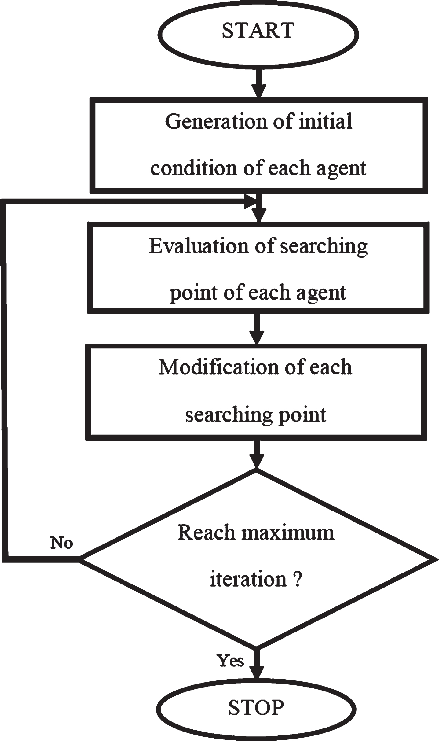
General flow chart of the PSO.

3 Mobile robot modeling

There are two types of models used in the simulation software for mobile robots:

3.1 Kinematics model

It is used to develop motion control strategy for mobile robots. This model is valid if the robot has low speed, light load, and low acceleration. The kinematics model of the robot velocity v and the angular velocity $\dot{θ}$ can be represented by the following matrix [19]: $[\begin{matrix} v \\ \dot{ϑ} \end{matrix}] = [\begin{matrix} r / 2 & r / 2 \\ r / 2 b & - r / 2 b \end{matrix}] [\begin{matrix} w_{r} \\ w_{l} \end{matrix}]$ (7)

Where r is the wheel radius, b is the half distance between the two wheels, θ is the heading angle, and W_r, W_l are the angular velocities of the right and left wheels respectively, with which speed is controlled.

3.2 Dynamic model

The mobile robot dynamic model used here is shown in Fig. 4. It consists of two wheels mounted on the same axis and a front passive wheel for balance. The two independent driving wheels are controlled by DC motors. The state variable of the robot is $x = [ν θ \dot{θ}]^{T}$ , the manipulated variable is u = [u_r u_l] ^T, and the output variable is y = [ν θ] ^T. This yields the following state-space equations [20]:

Fig.4

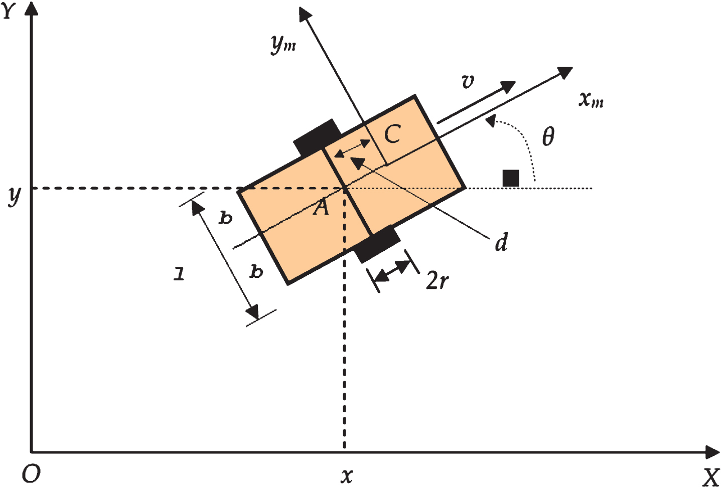
Dynamic model of mobile robots.

$\begin{matrix} x & = & A \dot{x} + Bu \\ y & = & Cx \end{matrix}$ (8)

Where A, B, and C are state space parameters given by: $A = [\begin{matrix} a_{1} & 0 & 0 \\ 0 & 0 & 1 \\ 0 & 0 & a_{2} \end{matrix}], B = [\begin{matrix} b_{1} \\ 0 \\ b_{2} \end{matrix} \begin{matrix} b_{1} \\ 0 \\ - b_{2} \end{matrix}], C = [\begin{matrix} 1 \\ 0 \end{matrix} \begin{matrix} 0 \\ 1 \end{matrix} \begin{matrix} 0 \\ 0 \end{matrix}]$ $\begin{matrix} a_{1} & = & - 2 c / ({Mr}^{2} + 2 I_{w}) \\ a_{2} & = & - 2 {cl}^{2} / (I_{v} r^{2} + 2 I_{w} l^{2}) \\ b_{1} & = & kr / ({Mr}^{2} + 2 I_{w}), b_{2} = krl / (I_{v} r^{2} + 2 I_{w} l^{2}) \end{matrix}$

The velocity and azimuth of the robot are controlled by manipulating the torques for the left wheel (ul) and the right wheel (ur). The different parameters of the dynamic model adopted in this work are defined in Table 1.

Table 1

Physical parameters of the robot dynamic model

Parameter	Definition	Value	Unit
I_v	Robot moment of inertia	10	Kg.m²
M	Robot mass	200	Kg
L	Distance between the 2 wheels	0.3	M
I_w	Wheel moment of inertia	0.005	Kg.m²
C	Viscous friction	0.05	Kg/s
R	Wheel radius	0.1	M
K	Driving gain factor	5	–

4 Motion control of the mobile robot

The control of mobile robot can be viewed as a hierarchical system of three stages: Motion planner, Motion controller, and Actuator driver. The highest level i.e. the motion planner is responsible of determining the path and velocity profiles that the robot should follow. The motion planning is done off-line or on-line. In off-line motion planner, the path to follow and velocity are determined beforehand while in the on-line motion planner; the robot modifies its movement by changing environmental factors. After the mobile robot knows its path that must follow, the controller at the second level takes on the task of making it get there. The actual position and velocity of the robot are measured by encoders and compared with the desired position and velocity generated by the motion planner. Based on the errors between the actual and desired states, the controller updates these values to get the desired position and velocity. The actuator driver receives input steering and velocity commands from the motion controller and produces the corresponding inputs to the motors of the mobile robot.

In this paper, the fuzzy logic is merged with APF to produce a FAPF scheme as a path planner. Again the fuzzy logic is used to design an intelligent motion controller. Hence, an FAPF-FC intelligent system is newly developed for mobile robots navigates without problems in dynamic environments.

5 Path planning schemes

The path planning scheme proposed in this work is the FAPF-FC/PSO that solves the problems of the classical APF method. The other schemes (APF-PID [16] and FAPF [13, 24]) given in this paper are designed for the sake of comparison with the FAPF-FC to prove the robustness of the proposed new system.

5.1 APF-PID scheme

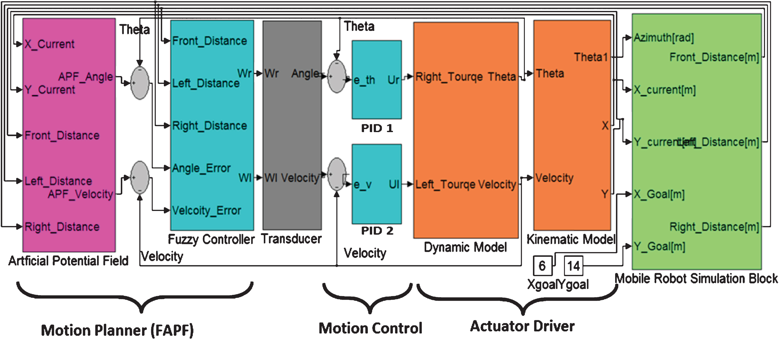
In this control model, the planning of mobile robot is done with classical APF and the motion control is done with two conventional PIDs to control velocity and azimuth. Based on the errors between the actual and desired states, the controller determines the steering angle and velocity that used to control the torques for the left and right wheels of the robot. Figure 5 shows the simulated block diagram for navigation of the robot using APF-PID.

Fig.5

Closed-loop APF-PID control system for navigation of mobile robot.

5.2 FAPF-FC/PSO proposed scheme

Since classical APF method suffers from local minima problems in some situations especially in dynamic and complex environments, fuzzy logic has features that proved to be an adequate tool to make some intelligent decisions that enable mobile robot to complete its task successfully. Hence, APF and fuzzy logic are combined to improve the performance of the path planning algorithm. The FLC takes input information (desired velocity and azimuth) from the APF model and at the same time senses the environment to look for any critical obstacles (static or dynamic) trying to avoid them as fast as possible. IR sensors are equipped with robot body to collect information about environment around mobile robot. Figure 6 shows the FAPF block diagram. APF plans the initial path or trajectory of mobile robot and starts executing it by following the direction of the total potential force. Once the fuzzy logic controller detects a high collision possibility, it will be forced to ignore the initial APF path and takes corresponding actions in terms of robot steering and velocity. That action is performed by turning robot to the right (increase left wheel velocity and decrease right wheel velocity) or left (increase right wheel velocity and decrease left wheel velocity) by activating the desired rules which perform collision avoidance to avoid obstacle, until new sensor readings dictate “not-possible” collision possibility then, the fuzzy logic controller takes into account the initial trajectory (i.e. velocity and direction of total potential field) as computed by the APF method which direct the mobile robot to goal.

Fig.6

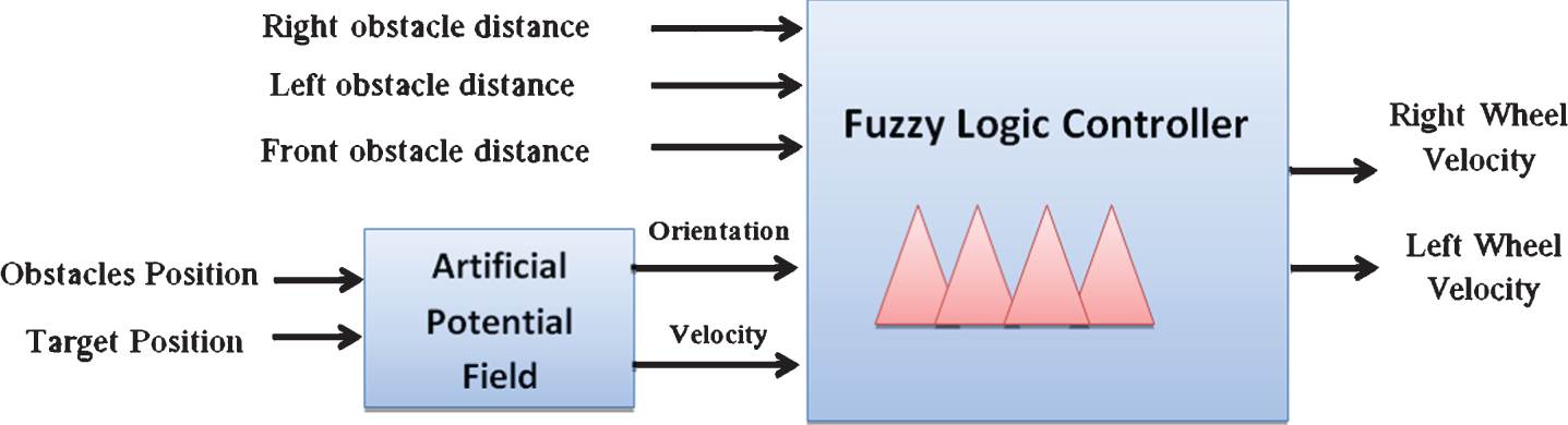
FAPF block diagram.

The APF is re-invoked every time the robot updates its position. FLC receives sensor information from three directions front, left, and right to guarantee collision avoidance with static and dynamic obstacles meanwhile following the trajectory. The flow chart of the FAPF is shown in Fig. 7. The axis correction module is activated by fuzzy controller if the current velocity and azimuth of robot do not coincide with the APF direction and velocity. This is done by taking the difference between current heading angle (θ_c) of mobile robot and angle generated by APF (θ_APF) and the difference between current velocity (V_c) of the mobile robot and velocity generated by APF (V_APF). The corresponding fuzzy rules of the fuzzy inference engine are activated to correct the direction and velocity of the robot towards its target. The outputs of the fuzzy controllers are the left and right wheel velocities “Wl” and “Wr” respectively. If the mobile robot does not find critical obstacles then it moves with the maximum possible speed in the direction of target with zero deviation of heading angle. This process continues, until the distance between mobile robot and goal (d_goal) is less than or equal to the minimum threshold distance (d_min). Two FLCs are used to control the mobile robot, one to control its velocity and the other to control its azimuth angle.

Fig.7

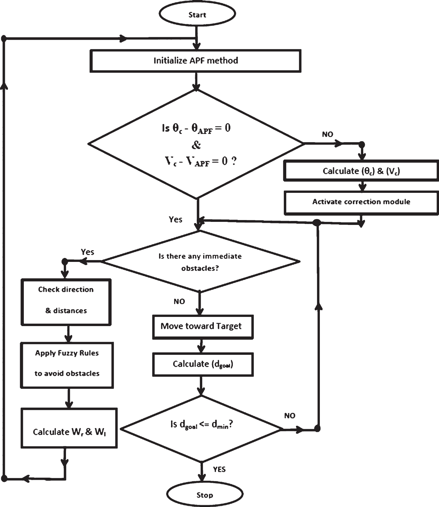
Flow chart of the FAPF.

These two parameters (velocity and azimuth) are controlled by manipulating the torque of the left and right wheels. The FLC inputs are error (e) and change of error (Δe) with triangular membership functions (MFs), and one output with sigmoid MF as shown in Fig. 8. The inputs and output of the FLC have 7 MFs (Negative Big “NB”, Negative Mid “NM”, Negative Small “NS”, Zero “ZO”, Positive Small “PS”, Positive Mid “PM”, Positive Big “PB”) with 6 parameters to tune resulting in 18 parameters. An optimization is introduced by PSO algorithm for tuning membership functions of two fuzzy logic controllers. Each controller has two inputs with triangular MF and one output with sigmoid MF, the first input is error and second input is change of error and output of each is control action. There are several methods to design membership functions, in this work we used the method in which to adjusts each parameters of MF in variable (e, Δe and output) alone and there parameters are cooperation with other two neighbors MFs. PSO attempts to optimize the scaling gains of the FLC inputs and output. Mean Square Error “MSE” criterion has been used as a fitness function to evaluate the performance of the system.

Fig.8

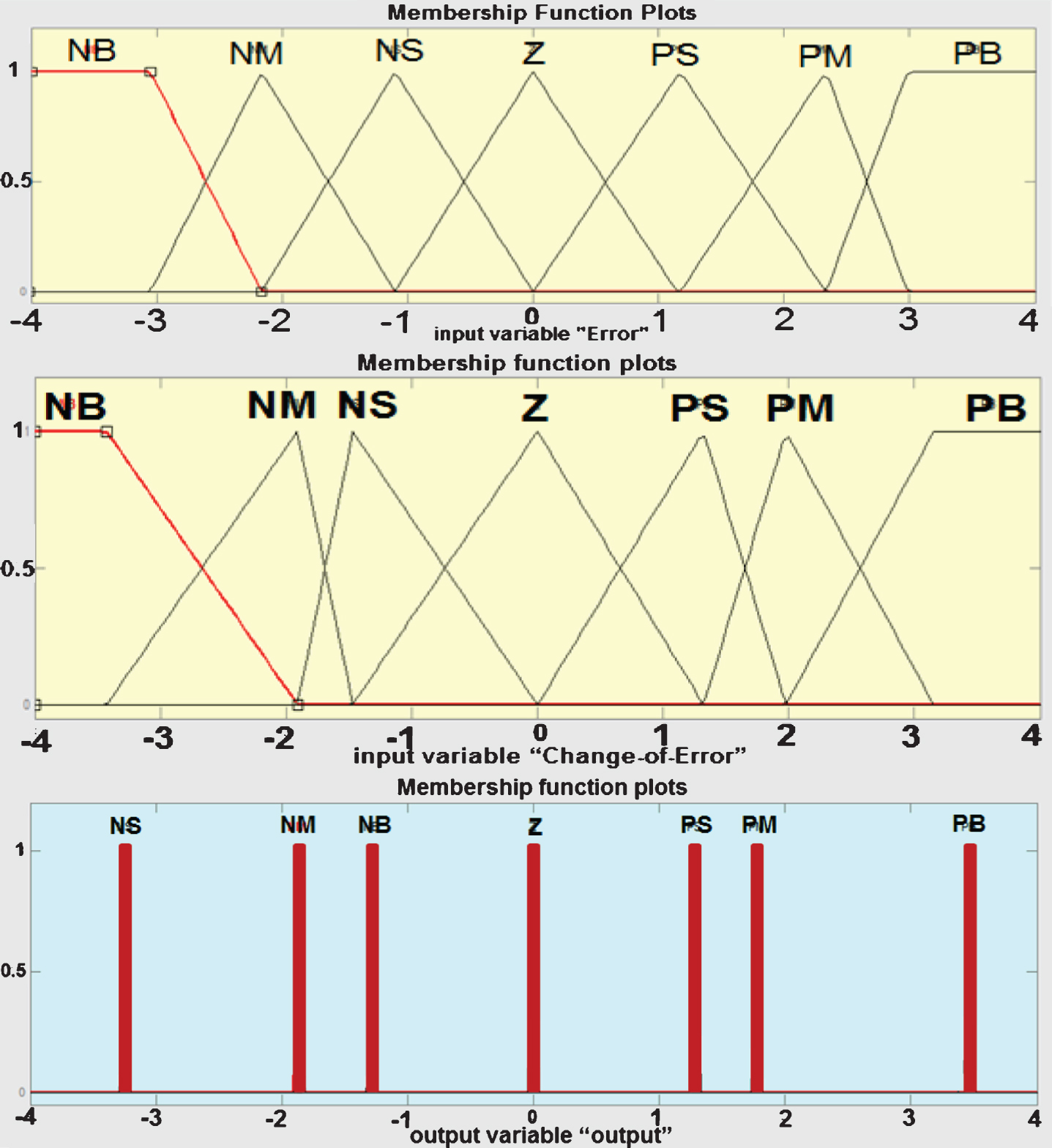
Optimized MFs for error (top), change of error (middle), and output (bottom) of the two FLCs.

The total number of scaling gains for the two FLCs is 6. Therefore, the total number of the parameters that should be optimized for the two FLCs is 24. The rules table consists of (7×7 = 49) rules given in Table 2. The rules table satisfies the three conditions for the rules formation, which are: complete, consistent, and continuous. The magnitude of the output control action is consistent with the magnitude of the input values. (i.e. in general, extreme input values (premise) result in extreme output values (consequent), mid-range input values in mid-range output values and small/zero input values in small/zero output values). The rule base is checked to give a smooth control surface. The simulated block diagram of the proposed FAPF-FC/PSO system for the robot navigation is shown in Fig. 9. It is displayed with a detailed block diagram for one fuzzy controller that designed for this system. The other fuzzy controller is exactly the same.

Table 2

Rule base for each of the two FLCs

e/Δe	NB	NM	NS	ZO	PS	PM	PB
NB	NB	NB	NB	NB	NM	NS	ZO
NM	NB	NB	NB	NM	NS	ZO	PS
NS	NB	NB	NM	NS	ZO	PS	PM
ZO	NB	NM	NS	ZO	PS	PM	PB
PS	NM	NS	ZO	PS	PM	PB	PB
PM	NS	ZO	PS	PM	PB	PB	PB
PB	ZO	PS	PM	PB	PB	PB	PB

Fig.9

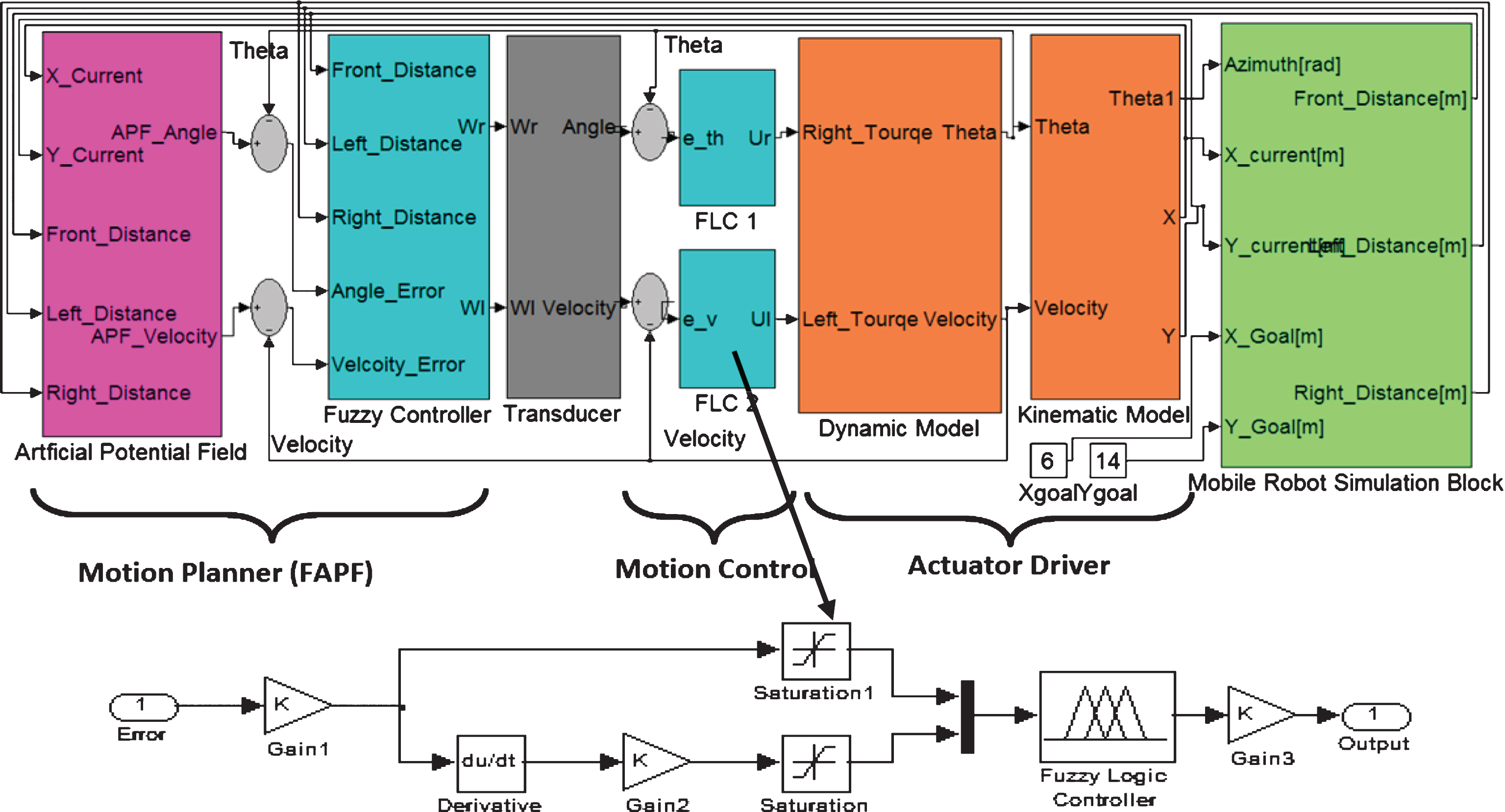
Closed-loop FAPF-FC/PSO control system for robot navigation.

5.3 FAPF-PID/PSO scheme

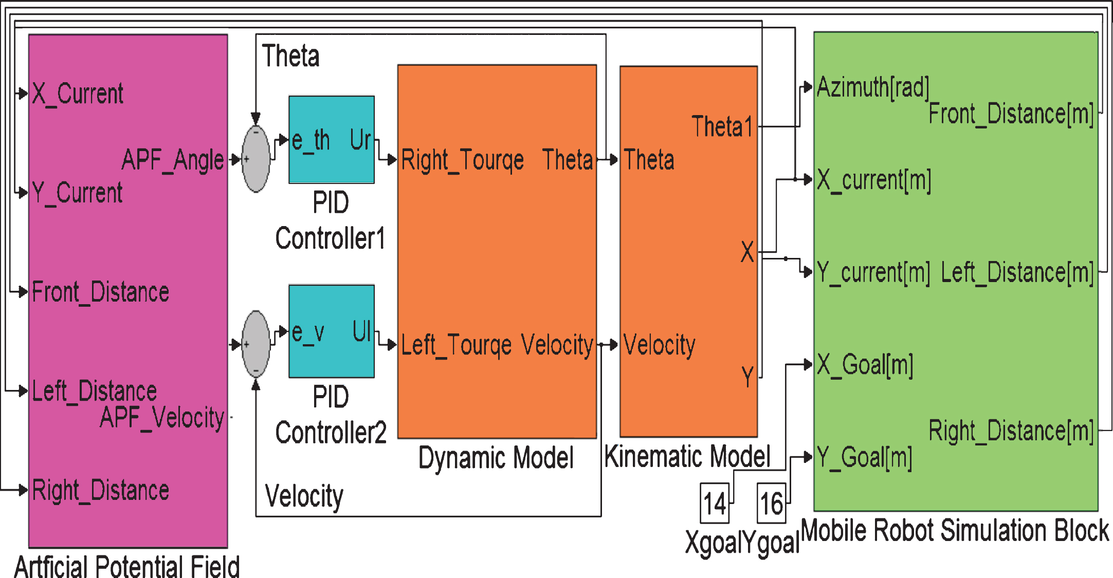
In this section, planning of the path of mobile robot using the FAPF with PID controllers tuned by PSO algorithm is given. The parameters of the two PID controllers and the MFs for the FLC that merged with the APF are optimized with the PSO. This scheme overcomes the problems of the classical APF, but with the PID controller, the system has less efficiency than that of the system with fuzzy controller. The robot needs much time and longer distance than that of the FAPF-FC to reach its goal. The simulated scheme of the FAPF-PID is shown in Fig. 10. The PSO algorithm is used to tune the two PID controllers.

Fig.10

Closed-loop FAPF-PID/PSO control system for robot navigation.

This is done by searching for their optimal value in the six dimensional search space, three dimensions specified for first controller (azimuth or angle controller) and another three dimensions for second controller (velocity controller), six parameters that will be tuned by PSO algorithm are [K_P1, K_I1, K_D1 ; K_P2, K_I2, K_D2]. By doing several experiments using different values for population size and number of iterations, it is observed that the following parameters values of PSO algorithm shown in Table 3 yield acceptable parameters for PID controllers to give a good performance to control the movement of mobile robot. Mean Square Error “MSE” criterion has been used as a fitness function to evaluate the performance of the system to compute the acceptable parameters by PSO algorithm.

Table 3

Parameters values of the PSO algorithm

Size of the swarm “no of birds”	100
Maximum iteration number	200
Dimension	6
PSO parameter c₁	2
PSO parameter c₁	2
W_max	0.9
W_min	0.3

6 Experimental setup

The robot chassis considered for experimental setup is a differential drive robot with two DC motors. Five Infrared (IR) sensors distributed on the robot body and two optical encoders each one gives 1000 pulses per 3 revolutions are included. The IR sensors are used to detect the position of the obstacles in the environment. The distribution of the IR sensors is shown in Fig. 11. To determine the robot current position, a simple and cheap odometer is used. Odometer operates by integrating incremental information over time.

Fig.11

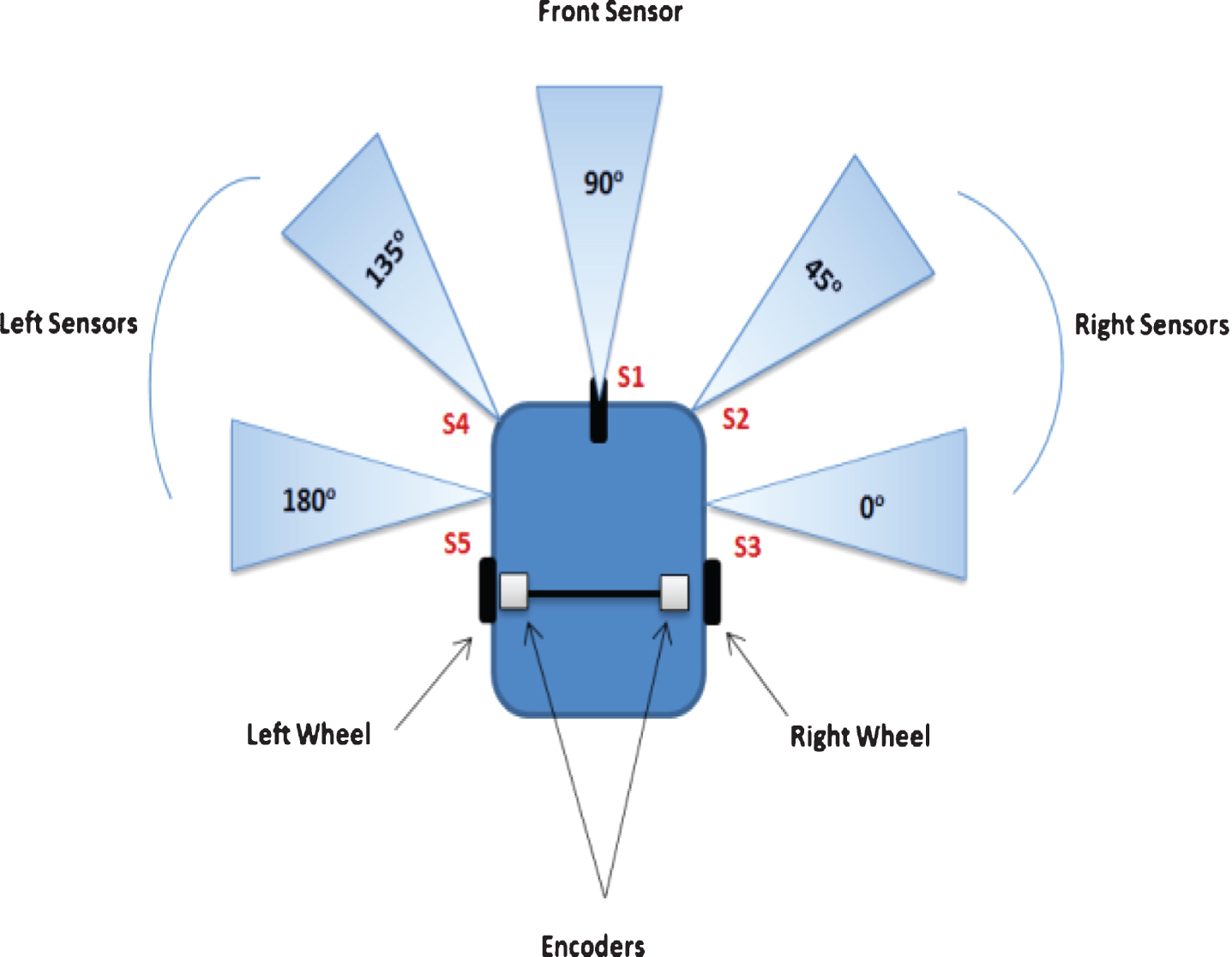
IR sensors configuration.

It uses wheel encoders to count the number of revolutions of each wheel. These encoders measure the distance that the robot traveled and its heading direction [21]. To calculate the current orientation and the distance traveled by the mobile robot since the last position calculation, we must first compute the incremental travel distance of the left and right wheels. The distances travelled by the left and right wheels (D_L and D_R) are computed by multiplying c_m by the left- and right-encoder counts respectively, where c_m is the conversion factor that translates encoder pulses or counts into linear wheel displacement and it is given by: $c_{m = 2 π r / C}$ (9)

C is the encoder resolution (in pulses or counts per revolution) and r is the wheel radius (in mm). The total distance (D_T) is then obtained by adding D_L and D_R divided by 2. The heading direction can be calculated by: $θ (rad) = {tan}^{- 1}$ (10)

l is the distance between the two wheels of the mobile robot. The mobile robot returns a 0 for global x-axis, a negative number for clockwise rotation, and a positive number for counter-clockwise rotation. The heading angle of the mobile robot ranges between (- π ∼ π) in the global frame. The position of the mobile robot in 2D Cartesian space is defined as:

$\begin{matrix} X_{position} & = & D_{T \times} sin (θ) \\ Y_{position} & = & D_{T \times} cos (θ) \end{matrix}$ (11)

The values of X_position, Y_position, and θ are calculated by odometer after tracking the position of robot continuously. X denotes lateral motion with negative values to the left and positive values to the right, Y denotes horizontal motion with negative values backwards and positive values forward, and θ denotes rotation in radian with zero angle for global X-axis coordinate, positive rotations to the right, and negative rotations to the left. The other hardware components of the system setup are microcontroller, H-bridge driver, and two DC motors. The proposed software model is embedded in the Arduino Mega 2560 microcontroller used for robot control. IR sensors, optical encoders, L298 N H-bridge driver are attached to the Arduino microcontroller. The speed and direction of motors are controlled by a pulse width modulation (PWM) signals coming from the Arduino to the H-bridge driver that controls the motors speed and direction. The FAPF-FC software model is reprogrammed in C and downloaded into the Arduino.

The embedded robot system is powered with rechargeable batteries that distribute the suitable powers to the various parts. The schematic diagram of the overall setup is shown in Fig. 12. This Arduino-based mobile robot is adopted for the practical test of the proposed path planning and motion control system.

Fig.12

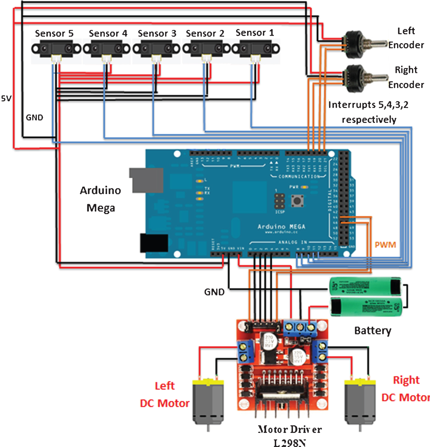
Schematic electronic diagram of the mobile robot.

7 Validation results

7.1 APF-PID software model

Special S-function is written to simulate the mobile robot platform with its IR sensors in its environment. The robot has three degrees of freedom represented by a posture Pc = (Xc, Yc, θ), where (Xc, Yc) is the robot current position and θ is the heading angle. Inputs to the simulation block are Xc, Yc, Xg, Yg, θ and time, where Xg and Yg is the target position. The S-function outputs are: Front_Distance (distance relative to front obstacle measured by sensor S1), Right_Distance (lowest distance relative to right obstacle measured by sensors S2 or S3), Left_Distance (lowest distance relative to left obstcle measured by sensors S4 or S5). The simulation block diagram is shown in Fig. 5. The parameters of the APF and the two PID controllers are found to be as shown in Table 4. The first simulation case shows the movement of robot from point (0,0) towards point (15,0) with one static obstacle located at (10.5,0). The robot stopped moving and cannot reach its target due to the occurrence of case 2 of local minima problem as shown in Fig. 13a.

Table 4
APF and PID parameters for robot navigation

ζ η d_o n $d_{goal}^{*}$

0.5 0.005 1.5 meter 1 1 meter

Velocity PID Parameters Angle PID Parameters

Kp = 32 Kp = 20

Ki = 1.33 Ki = 0.2

Kd = 2.9 Kd = 2.8

ζ	η	d_o	n	$d_{goal}^{*}$
0.5	0.005	1.5 meter	1	1 meter
Velocity PID Parameters	Angle PID Parameters
Kp = 32	Kp = 20
Ki = 1.33	Ki = 0.2
Kd = 2.9	Kd = 2.8

The second simulation case shows the environment in which the robot intended to move from start point (0,0) to target point (4.5,9.5) with one static obstacle located at (4,8.5) in the environment. Simulation result shows how the “goals non-reachable with obstacle nearby” problem occurs and causes local minima because the goal is located within the active region of the obstacle as shown in Fig. 13b. Again, the robot is stopped and never reaches its goal point. The third simulation case shows the environment in which the robot would move from start point (0,0) to target point (14,16) with an obstacle organized as a U-shaped. The mobile robot fails to avoid U-shaped obstacle and being trapped and cannot reach to goal point as shown in Fig. 13c. The cases shown in Fig. 13 are the most commonly problems that occur with conventional APF path planning algorithm.

Fig.13

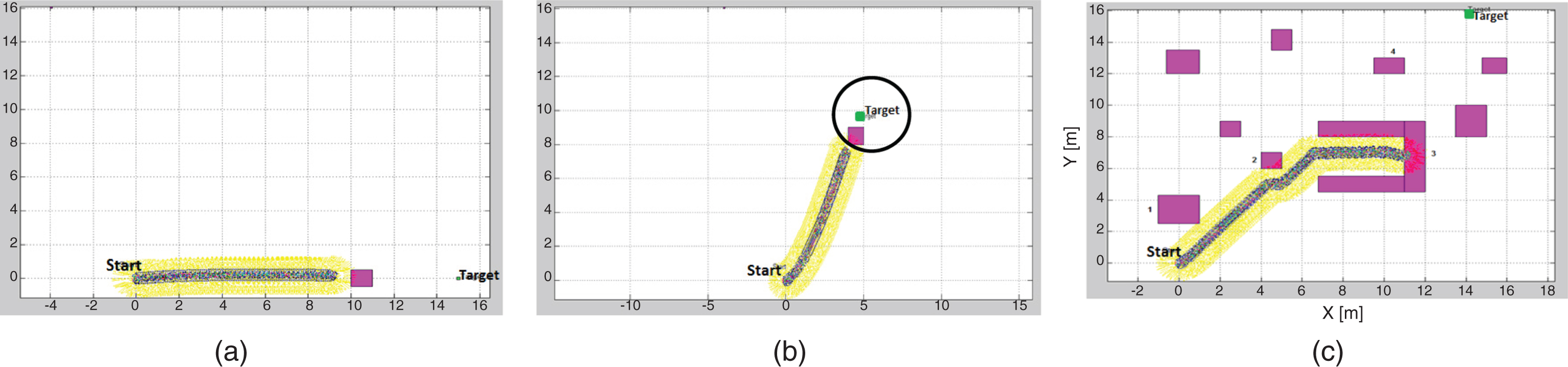
Mobile robot navigation with APF-PID scheme in different environments showing the local minima problems.

7.2 FAPF-PID/PSO software model

The path planning and control of mobile robot using the proposed FAPF method with PID controller optimized with PSO algorithm is presented. The simulation block diagram is given in Fig. 10. The first simulation environment for robot navigation shows that the robot faces a difficult situation when navigates in a complex U-shaped structure but it succeeded to avoid it and reaches to its goal point as shown in Fig. 14. The mobile robot is tested with and without load to check the effect of disturbance and hence proving its robustness. Table 5 shows the elapsed times and the travelled distance of the mobile robot taking into consideration a load of 50Kg.

Table 5
Time and distance calculations of the robot navigation in static environment with FAPF-PID scheme

Elapsed time (sec) FAPF + PID/PSO FAPF + PID/PSO

to avoid: (with load)

obstacle 1 0 0

obstacle 2 0 0

obstacle 3 U-shape 2.6 2.65

obstacle 4 0.3 0.3

Total time 5.71 5.72

Total distance (m) 34.8 34.98

Elapsed time (sec)	FAPF + PID/PSO	FAPF + PID/PSO
obstacle 1	0	0
obstacle 2	0	0
obstacle 3 U-shape	2.6	2.65
obstacle 4	0.3	0.3
Total time	5.71	5.72
Total distance (m)	34.8	34.98

Fig.14

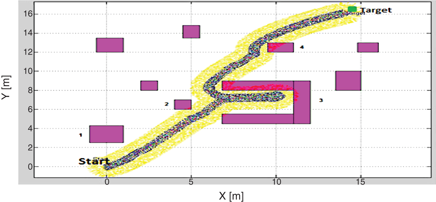
Mobile robot navigation using FAPF-PID control scheme.

It is clear that the effect of load is insignificant, means that the navigation is robust with and without load. Figure 15 illustrates the velocity, azimuth, and errors of the mobile robot navigation.

Fig.15

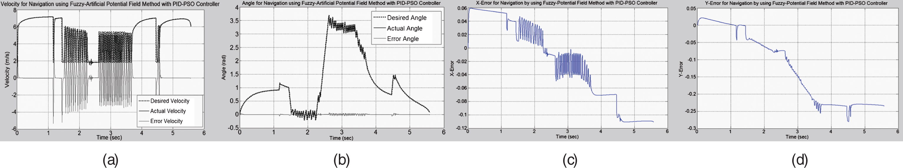
a) Velocity calculation of 1st PID b) Azimuth calculation of 2nd PID c,d) X & Y errors of robot movement of the FAPF-PID system.

Fig.16

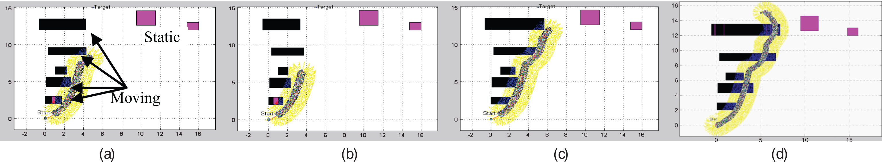
Robot navigation using FAPF-PID scheme in environment wih static and dynamic obstacles.

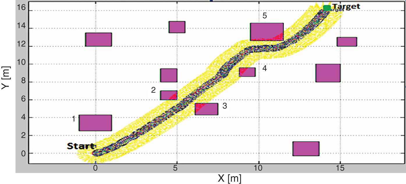
The second environment is built with dynamic (moving) obstacles. In this environment, the robot is moved from start point (0,0) to target point (5,15) with static and dynamic obstacles of different sizes and shapes spread in the environment. In spite of that the mobile robot succeeded to avoid the dynamic obstacles, but its movement is less smooth and sometimes there is a fluctuation in the robot movement as shown in Fig. 16. Table 6 shows the elapsed time and the total travelled distance for this environment. The velocity, azimuth, and error of the mobile robot navigated in this environment are shown in Fig. 17.

Table 6

Time and distance calculations of the robot navigation in dynamic environment with FAPF-PID scheme

Elapsed time (sec)	FAPF + PID-PSO	FAPF + PID/PSO
to avoid:		(with load)
obstacle 1	0.1	0.1
obstacle 2	0.1	0.1
obstacle 3	0.1	0.1
obstacle 4	0.3	0.3
obstacle 5	0.4	0.4
Total Elapsed time	2.7	2.72
Total distance (m)	16.2	16.32

Fig.17

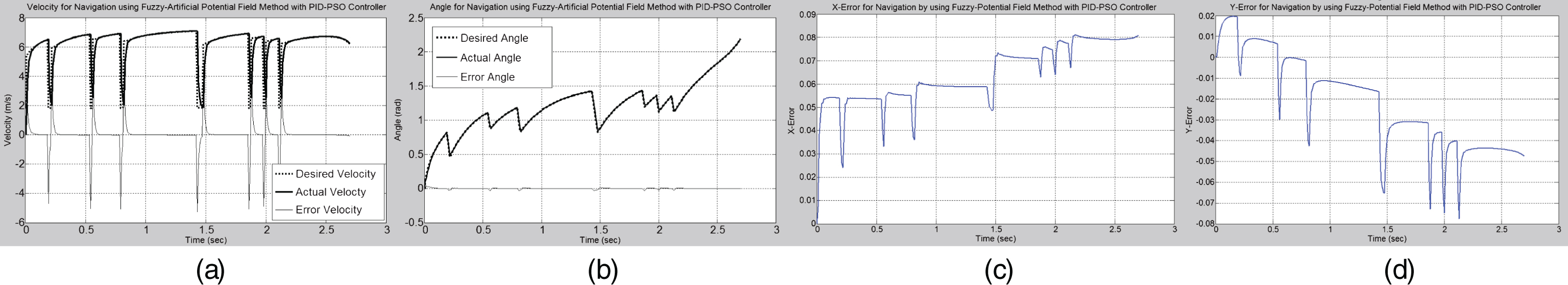
a) Velocity calculation of 1st PID b) Azimuth calculation of 2nd PID c,d) X & Y errors of robot movement of the FAPF-PID system.

7.3 FAPF-FC/PSO software model

The first simulation model for the mobile robot movement from point (0,0) to point (14,16) using FAPF for path planning and fuzzy controller for motion control is presented in Fig. 18. Figure 19 illustrates the velocity, azimuth, and error of mobile robot moving in this environment. Table 7 shows the elapsed time and total travelled distance of the mobile robot moving in this environment.

Fig.18

Robot navigation using FAPF-FC/PSO scheme in static environment.

Fig.19

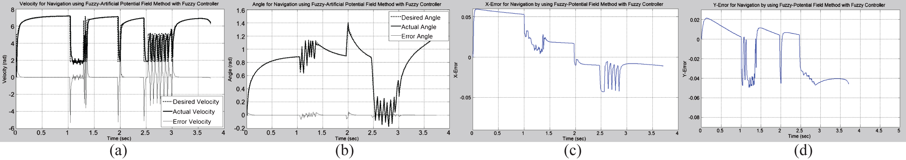
a) Velocity calculation of 1st FLC b) Azimuth calculation of 2nd FLC c,d) X & Y errors of robot movement of the FAPF-FC system.

Table 7

Time and distance calculations of the robot navigation in static environment with FAPF-FC scheme

Elapsed time (sec)	FAPF-FC	FAPF-FC
to avoid:		(with load)
obstacle 1	0	0
obstacle 2	0.4	0.4
obstacle 3	0.4	0.4
obstacle 4	0.2	0.2
obstacle 5	0.5	0.5
Total Elapsed Time	3.5	3.6
Total distance (m)	21	21.6

Table 8

Time and distance calculations of the robot navigation in static environment with FAPF-PID scheme

Elapsed time (sec)	FAPF-PID	FAPF-PID
to avoid:		(with load)
obstacle 1	0	0
obstacle 2	0.4	0.4
obstacle 3	0.4	0.4
obstacle 4	0.2	0.2
obstacle 5	0.5	0.5
Total Elapsed Time	3.7	3.8
Total distance (m)	22.2	22.8

If the same simulation environment of Fig. 18 is repeated but with FAPF-PID scheme, the results for elapsed time and total travelled distance are obtained and given in Table 8. It is noticed that the total elapsed time and total travelled distance for FAPF-FC system is better than that of the FAPF-PID system. Of course, for long robot movement, the significance will be greater.

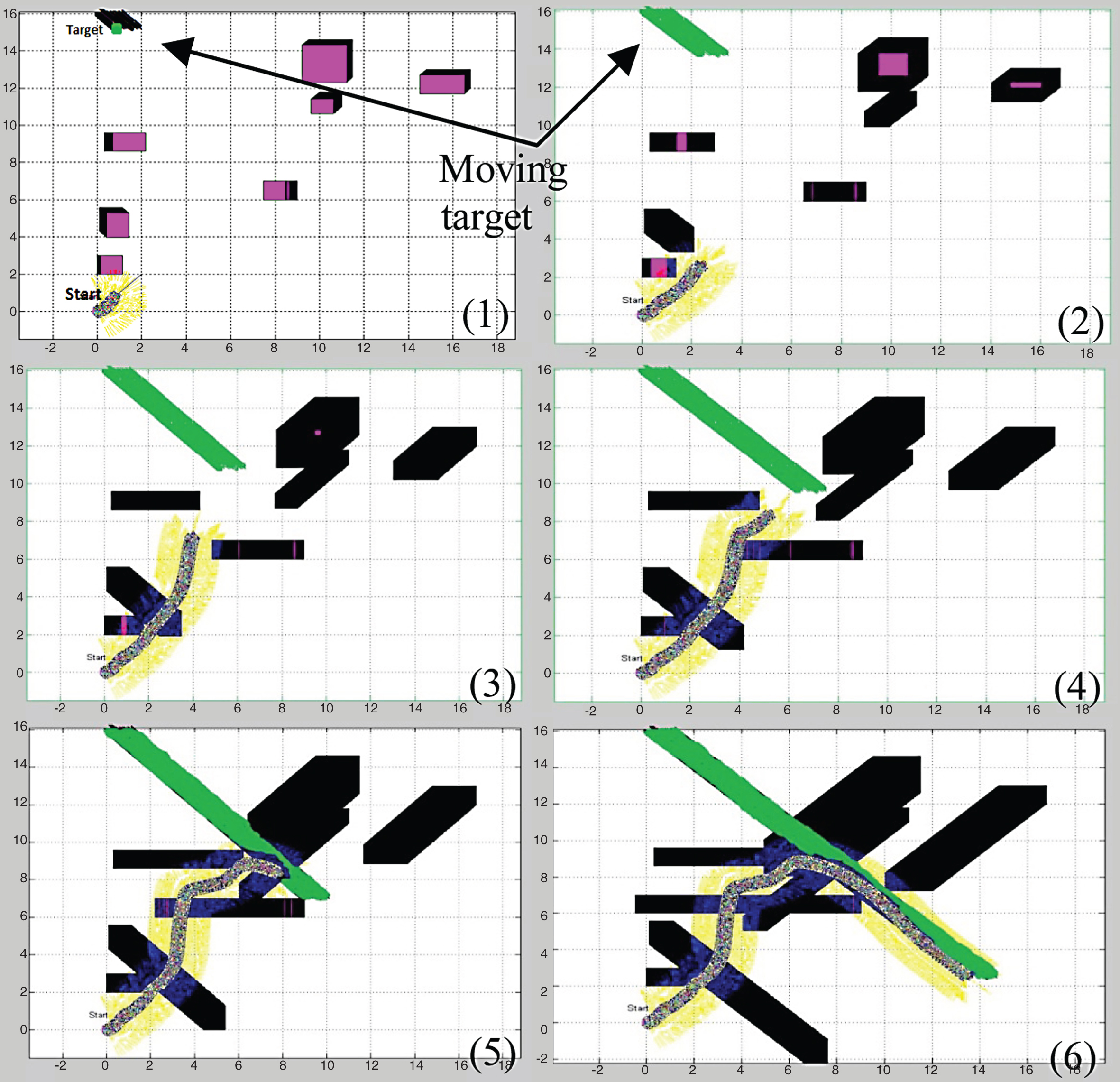
To test the performance of the robot navigation with FAPF-FC in totally dynamic environment (all obstacles and target are moving), a simulation model is built. The robot moves from start point (0,0) to a moving target that is moving randomly starting from point (0,16) as shown in Fig. 20. The simulation showed that the mobile robot navigated in the dynamic environment and reached to the moving target successfully with smooth and fast reaction movement.

Fig.20

Real robot with FAPF-FC embedded controller navigates in real environmnet.

Fig.21

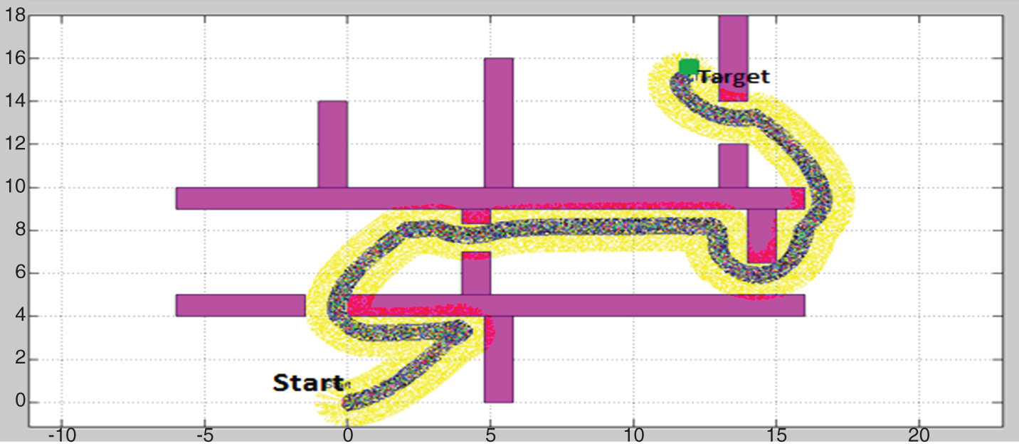
Robot navigation using FAPF-FC/PSO scheme in a maze environment.

Also, to test the performance of the robot navigation using FAPF-FC in an environment configured as a maze, a simulation model for movement from point (0,0) to point (12,15) is made as in Fig. 21. This type of environments is considered as one of the most complex environments that the mobile robot may face. The simulation showed that the mobile robot navigates successfully inside the maze and reached to the desired target point with smooth and fast reaction motion.

7.4 Experimental tests

To prove that the FAPF algorithm works appropriately, the mobile robot is tested in real environment with many different obstacles. This environment, which is considered as a Cartesian coordinate system, contains four different obstacles as shown in Fig. 22. The test showed that the designed robot succeeded in avoiding obstacles and reached to the goal point with small position error due to the little accuracy of the used shaft encoders. This error can be reduced if a high accuracy encoders or GPS is used.

Fig.22

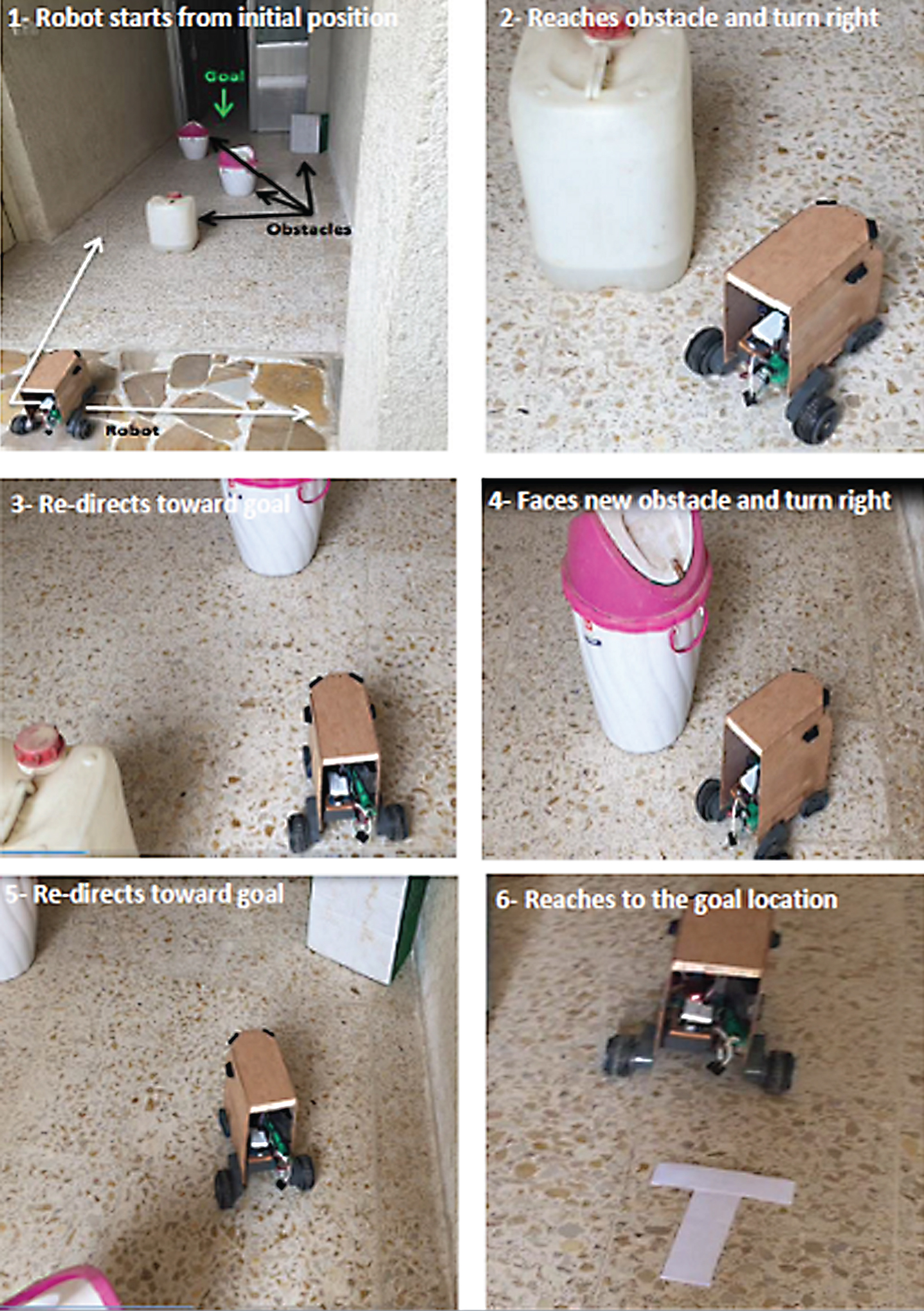
Real robot with FAPF-FC embedded controller navigates in real environment.

8 Conclusions

APF method is a fast and efficient method for path planning of mobile robots. The traditional APF method sometimes causes an inefficient path planning or generates a local minimum. The proposed method in this paper combines APF with fuzzy logic to solve the problems of traditional method and enhances the performance of path planning of mobile robot in complex and dynamic unknown environments. The proposed method is introduced with two schemes; the first one is introduced with PID motion controller. In the second scheme the proposed method is introduced with fuzzy logic motion controller. In spite of that the two schemes produce good results but the FAPF-FC made the mobile robot capable of reaching its target efficiently with less time and distance, fast reaction with obstacle nearby, and no fluctuation around obstacle. The PSO algorithm is used for tuning/optimizing the parameters of PID controller parameters, membership functions of FLC and the APF parameters. The navigation of mobile robot is tested by using simulated environments. The test included many cases of path planning schemes in different static and dynamic environments. The simulation results showed that the FAPF-FC results in shorter and smoother path for mobile robot navigation and the mobile robot can react much faster in all static and dynamic environments that contain moving target and obstacles and can avoid them automatically and reach to its target. The robot is implemented practically and tested experimentally to prove the effectiveness and robustness of the proposed system. It could navigate properly and reach its target with a small position error due to the low accuracy of the shaft encoder.

Footnotes

References

Kala

, Shukla

and Tiwari

, Fusion of probabilistic A* algorithm and fuzzy inference system for robotic path planning, Springer, Artificial Intelligence Review 33(4) (2010), 307–327.

Fuji

, Xiang

, Tazaki

and Levedahl

, Trajectory planning for automated parking using multi-resolution state roadmap considering non-holonomic constraints, Proceedings of the IEEE conference on Intelligent Vehicles Symposium, Dearborn, 2014, pp. 407–413.

Donald Smart

and Kiebling

, Effective reinforcement learning for mobile robots, IEEE International Conference on Robotics & Automation, USA, 2002, pp. 3404–3410.

Chiang

Hao-Tien

, Malone

and Lesser

, Path-guided artificial potential fields with stochastic reachable sets for motion planning in highly dynamic environments, IEEE International Conference on Robotics & Automation (ICRA), USA, 2015, pp. 2347–2354.

Panigrahi

P.K.

and Sahoo

, Navigation of autonomous mobile robot using different activation functions of wavelet neural network, IEEE International Conference on Convergence of Technology (I2CT), India, 2014, pp. 1–6.

Seraji

and Howard

, Behavior-based robot ngation on challenging terrain: A fuzzy logic approach, IEEE Trans on Robotics & Automation 18(3) (2002), 208–321.

Khatib

, Real-time obstacle avoidance for manipulators and mobile robots, International Journal of Robotic Research 5 (1986), 90–98.

Chengqing

, Ang

M.H.

Jr , Krishnan

and Yong

, Virtual obstacle concept for local-minimum-recovery in potential-field based navigation, IEEE International Conference on Robotics & Automation, San Francisco, 2000.

S.S.

and Cui

Y.J.

, Dynamic motion planning for mobile robots using potential field method, Autonomous Robots 13 (2002), 207–222.

10.

S.S.

and Cui

Y.J.

, New potential functions for mobile robot path planning, IEEE Transactions on Robotics and Automation 16 (2002), 615–620.

11.

Wang

Mei

, Su

Zhiyong

, Tu

Dawei

and Lu

Xichang

, A hybrid algorithm based on artificial potential field and BUG for path planning of mobile robot, IEEE International Conference on Measurement, Information and Control (ICMIC), China, vol. 02, 2013, pp.1393–1398.

12.

Vadakkepat

, Tan

K.C.

and Ming-Liang

, Evolutionary artificial potential fields and their application in real time robot path planning, Congress on Evolutionary Computation 1 (2000), 256–263.

13.

Weijun

, Rui

and Chongchong

, A study on soccer robot path planning with fuzzy artificial potential field, International Conference on Computing, Control and Industrial Engineering, Vol. 1, 2010, pp. 386–390.

14.

Hamani

and Hassan

, Mobile robot navigation in unknown environment using improved APF method, International Arab Conference on information Technology, 2012.

15.

Chunshu

, Cui

Genqun

and Lu

Haifeng

, The design of an obstacle avoiding trajectory in unknown environment using potential fields, IEEE International Conference on Information and Automation (ICIA), China, 2010, pp. 2050–2054.

16.

Gue

, Gao

and Cui

, Path planning of mobile robot based on improved potential field, Information Technology Journal 12(11) (2013).

17.

Gupta

, Behera

and Venkatesh

K.S.

, PSO based modeling of Takagi-Sugeno fuzzy motion controller for dynamic object tracking with mobile platform, IEEE the International Multi Conference on Computer Science and Information Technology, Poland, Vol. 5, 2010, pp. 37–43.

18.

Kim

Jeong-Jung

and Lee

Ju-Jang

, Trajectory optimization with particle swarm optimization for manipulator motion planning, Proceedings of IEEE Transactions on Industrial Informatics, South Korea 11(3) (2015), 620–631.

19.

Mester

, Motion control of wheeled mobile robots, SISY 2006 4th Serbian-Hungarian Joint Symposium on Intelligent Systems.

20.

Peng

, Wang

and Sun

, Trajectory tracking control for mobile robot using recurrent fuzzy cerebellar model articulation controller, Neural Information Processing–Letters and Reviews 11(1) (2007).

21.

Borenstein

, Control and kinematic design of multi-degree-of-freedom robots with compliant linkage, IEEE Trans, on Robotics and Automation 11(1) (1995), 21–35.

22.

Kumar

, Dayal

and Kumar

P.A.

, Navigation technique to control several mobile robots, International Journal of Knowledge-based and Intelligent Engineering Systems 10(5) (2006), 387–401.

23.

Ramanathan

, Periasamy

V.M.

, Pushpavanam

and Natarajan

, Particle swarm optimization of hardness in nickel diamond electro composites, International Scientific Journal 1(4) (2009), 232–236.

24.

Song

and Liu

, Mobile robot path planning based on dynamic fuzzy artificial potential field method, International Journal of Hybrid Information Technology 5(4) (2012).

Mobile robot navigation using PSO-optimized fuzzy artificial potential field with fuzzy control

Abstract

Keywords

1 Introduction

2 Problem statement

3.1 Kinematics model

5 Path planning schemes

5.1 APF-PID scheme

7.1 APF-PID software model

Table 4 APF and PID parameters for robot navigation ζ η do n d goal * 0.5 0.005 1.5 meter 1 1 meter Velocity PID Parameters Angle PID Parameters Kp = 32 Kp = 20 Ki = 1.33 Ki = 0.2 Kd = 2.9 Kd = 2.8

Footnotes

References

Table 4
APF and PID parameters for robot navigation

ζ η d_o n $d_{goal}^{*}$

0.5 0.005 1.5 meter 1 1 meter

Velocity PID Parameters Angle PID Parameters

Kp = 32 Kp = 20

Ki = 1.33 Ki = 0.2

Kd = 2.9 Kd = 2.8