A Clinically-Translatable Machine Learning Algorithm for the Prediction of Alzheimer’s Disease Conversion in Individuals with Mild and Premild Cognitive Impairment

Abstract

Background:

Available therapies for Alzheimer’s disease (AD) can only alleviate and delay the advance of symptoms, with the greatest impact eventually achieved when provided at an early stage. Thus, early identification of which subjects at high risk, e.g., with MCI, will later develop AD is of key importance. Currently available machine learning algorithms achieve only limited predictive accuracy or they are based on expensive and hard-to-collect information.

Objective:

The current study aims to develop an algorithm for a 3-year prediction of conversion to AD in MCI and PreMCI subjects based only on non-invasively and effectively collectable predictors.

Methods:

A dataset of 123 MCI/PreMCI subjects was used to train different machine learning techniques. Baseline information regarding sociodemographic characteristics, clinical and neuropsychological test scores, cardiovascular risk indexes, and a visual rating scale for brain atrophy was used to extract 36 predictors. Leave-pair-out-cross-validation was employed as validation strategy and a recursive feature elimination procedure was applied to identify a relevant subset of predictors.

Results:

16 predictors were selected from all domains excluding sociodemographic information. The best model resulted a support vector machine with radial-basis function kernel (whole sample: AUC = 0.962, best balanced accuracy = 0.913; MCI sub-group alone: AUC = 0.914, best balanced accuracy = 0.874).

Conclusions:

Our algorithm shows very high cross-validated performances that outperform the vast majority of the currently available algorithms, and all those which use only non-invasive and effectively assessable predictors. Further testing and optimization in independent samples will warrant its application in both clinical practice and clinical trials.

Keywords

Alzheimer’s disease clinical prediction rule machine learning mild cognitive impairment personalized medicine

INTRODUCTION

Alzheimer’s disease (AD) is a neurodegenerative disease characterized by progressive loss of memory and functional abilities that leads to severe dementia and eventually death. It is the most common neurodegenerative disease and currently affects 47 million people worldwide, being the top cause for disabilities in later life. The global cost of AD and dementia is estimated to be $818 billion, which is nearly 1% of the entire world’s gross domestic product. These numbers are projected to increase, with a global expected cost of $2 trillion by 2030 and more than 131 million people suffering from this disorder by 2050 [1].

No cure or disease modifying treatment is currently available for AD and current treatment regimens only provide symptomatic relief [2]. By the time AD is clinically diagnosed, there is considerable multi-system degeneration that has occurred within the brain. As such, emerging treatments will likely have the greatest impact when provided at the earliest possible stage of the disease process [3, 4].

Therefore, the prompt identification of subjects truly at high risk of developing AD is a crucial issue still without a solution.

Mild cognitive impairment (MCI) is a condition characterized by changes in cognitive capabilities beyond what is expected for the subject’s age and education that are sufficiently mild that they do not interfere significantly with its daily activities. Individuals with such condition are at high risk of converting to dementia and especially AD in the next few years (20–40% of conversion rate by three years, with a lower rate evidenced in epidemiologic samples than in clinical ones [5, 6]).

Furthermore, even subjects with an intermediate state between normal cognition and MCI, i.e., the so called premild cognitive impairment (PreMCI) stage [7], are more likely to progress to a formal diagnosis of MCI or dementia within a two- to three-year period, and this might represent the earliest clinically definable stage of AD [8].

However, some subjects with MCI have shown to remain stable over years or even to recover to cognitively normal with no further progression to AD. This holds even more true for subjects with PreMCI than for those with MCI [8]. Different health problems other than neurodegenerative diseases can cause transient MCI and PreMCI conditions and these do not necessarily lead to AD [9]. Thus, sole reliance on these precursor conditions are not enough to provide a precise identification of those subjects at true risk of later developing AD.

Beyond MCI and preMCI, several attempts to identify subject’s characteristics that may improve the prediction of progression to AD have been done. Investigations have regarded a vast variety of potential predictors, such as sociodemographic and clinical characteristics, cognitive performances, neuropsychiatric symptomatology, cardiovascular indexes, dietary and life habits, structural and functional neuroimaging investigations, gene typization, and several biomarkers assessed both in the cerebrospinal fluid and peripherally [10 –16].

It is increasingly recognized that better predictive capability can be achieved by models that simultaneously exploit the information coming from several predictors, and machine learning can be used to create such models. This is a fast-growing field at the crossroads of computer science, engineering, and statistics “that gives computers the ability to learn without being explicitly programmed” [17]. Machine learning techniques use known training examples to create algorithms able to provide the best possible prediction when applied to new cases whose outcome is still unknown. Machine learning has been applied in the attempt to predict MCI-AD conversion in more than 50 published studies. Different combinations of the above-mentioned predictors were applied to various machine learning techniques in the attempt to predict conversion from MCI to dementia from one year to even five years after the baseline assessment. The results achieved vary broadly among studies, ranging from some that achieved performances just above the chance to a few showing high accuracy levels [18 –26].

Despite this huge research effort, no gold-standard algorithm is available to predict progression in those at risk for AD and clinical translation is still lacking. All the “top performing” algorithms have not been tested in further independent samples thus far, and, in addition, certain predictors employed by some models may represent a significant barrier to their clinical adoption due to their high costs and/or invasiveness (e.g., fludeoxyglucose positron emission tomography scans or lumbar puncture).

Considering all the above-mentioned issues, the current study aims to be the first step in the development of a clinically-translatable algorithm for the identification of the conversion to AD in subjects with either MCI or PreMCI. To be quickly adoptable in clinical practice, the algorithm should include only non-invasive predictors that are either already routinely assessed or effectively introducible in clinical practice, and achieve a high predictive accuracy. Considering the evidence available so far, we hypothesize that the information provided by sociodemographic characteristics, clinical and neuropsychological tests, cardiovascular risk indexes, and clinician-rated level of brain atrophy might allow achieving this. In this investigation, a series of machine learning algorithm will be developed and cross-validated within a sample of patients with either MCI/PreMCI whose diagnostic follow-up was available for at least three years after the baseline assessment. Out-of-the-sample testing of the best algorithm in independent samples of MCI/PreMCI patients will be performed in a further phase.

MATERIALS AND METHODS

Subjects

Data regarding 90 subjects with MCI and 94 subjects with PreMCI at baseline and with available diagnostic follow-up assessments for at least three years were included in the study.

These are part of a dataset that collects several patients recruited in a study investigating longitudinal changes associated with MCI and normal aging, which involved community volunteers as well as subjects recruited from the Memory Disorders Clinic at the Wien Center for Alzheimer’s disease, the Memory Disorders at Mount Sinai Medical Center, Miami, Beach, Florida, and the community and memory disorders center at the University of South Florida which were collaborative partners in an Alzheimer’s Disease Research Center (ADRC). All subjects at each of the sites had a common clinical and neuropsychological battery as described below.

Considering the final aim of developing a predictive algorithm to be used in clinical practice, no other inclusion or exclusion criteria were applied beyond these diagnostic criteria. Subjects were classified as converters to probable AD (cAD; n = 48, 26.1%) if they presented a Dementia syndrome by DSM-IV-TR criteria [27] during at least one of the follow-up assessments occurred within three years from the baseline investigation, and satisfied the National Institute of Neurological and Communicative Disorders and Stroke/Alzheimer’s Disease and Related Disorders Association criteria for AD [28]. Otherwise they were classified as non-converters to AD (NC; n = 136, 73.9%).

The study was conducted with the ethical standards of the relevant national and institutional committees on human experimentation and with the Helsinki Declaration of 1975, as revised in 2008. All subjects gave their written informed consent to the use of their clinical data for scientific research purposes.

Feature extraction

Considering our aim to employ only predictors that are non-invasive and that are either already routinely assessed or cost-effectively introducible in clinical practice, we decided to focus on information available in our dataset that regard diagnostic subtypes, sociodemographic characteristics, clinical and neuropsychological test scores, cardiovascular risk indexes, and levels of medial temporal lobe brain atrophy in the hippocampus (HPC), entorhinal cortex (ERC), and perirhinal cortex (PRC) as assessed by a clinician-rated Visual Rating Scale (VRS) [29].

Among all the variables related to these domains, some of them were not assessed in all recruited subjects. Variables that had more than 20% missing values in either the cAD or NC groups were discarded. The following pieces of information were finally used.

Sociodemographic characteristics

Gender, age (in years), and years of education calculated by years of schooling and highest degree obtained.

MCI subgroups

Subjects were classified as MCI if they presented subjective memory complaints by the participant and/or or collateral informant, evidence of decline from clinical history and evaluation. All of the MCI patients had a global Clinical Dementia Rating (CDR) score [30] of 0.5. Those who had one or more memory measures (including the Hopkins Verbal Learning Test Revised, the Fuld Object Memory Evaluation, Logical Memory Delay and Visual Reproduction of the WMS-IV, Trial Making Test, Category Fluency, Letter Fluency and Block Design of the Wechsler Adult Intelligence Scale – Version 3) 1.5 standard deviation or greater below expected normative values were defined as belonging to the amnestic mild cognitive impairment (aMCI) subgroup. MCI subjects with non-memory impairment only were defined as non-amnestic mild cognitive impairment (non-aMCI).

PreMCI subgroups

As defined by Loewenstein and colleagues [8], those individuals who had a global CDR of 0 but had memory or non-memory neuropsychological deficits as described above were diagnosed as Premild Cognitive Impairment – neuropsychological subtype (PreMCI-np). Participants who obtained a global CDR of 0.5 and had within normal limits performance on neuropsychological testing were classified as Premild Cognitive Impairment – clinical subtype (PreMCI-cl).

Clinical scales

The CDR [30] is a 5-point scale (0 = none; 0.5 = very mild, 1 = mild, 2 = moderate, 3 = severe) used to characterize six domains of cognitive and functional performance in AD and related dementias: Memory, Orientation, Judgment & Problem Solving, Community Affairs, Home & Hobbies, and Personal Care. The rating is obtained through a semi-structured interview of the patient together with other informants (e.g., family members). The global score was used in the analyses. The memory sum score of a modified informant-based version of CDR (ModCDR-M) was also available and used (range 0–12) [31]. The Geriatric Depression Scale (GDS) is a 30-item yes-no self-report assessment used to identify depression in the elderly [32] and the total score was included in the current analyses (range 0–30).

Visual Rating Scale for brain atrophy

HPC, ERC, and PRC atrophy levels were assessed with a 0–4 VRS [29]. This is an adaptation from the original Scheltens’ VRS for the global assessment of medial temporal atrophy [33]. VRS ratings for HPC, ERC, and PRC were performed in each hemisphere on a magnetic resonance imaging (MRI) image of a standardized coronal slice, perpendicular to the line joining the anterior and posterior commissures, intersecting the mammillary bodies and on adjacent slices. All these 6 VRS measures were separately included as predictors in this study. Ratings are based on a five-point scale: 0 = no atrophy, 1 = minimal atrophy, 2 = mild atrophy, 3 = moderate atrophy, and 4 = severe atrophy. A computer interface provides a library of reference images defining the anatomical boundaries of each brain structure and depicting different levels of atrophy. The whole rating usually takes 5 to 6 minutes per subject [34] and excellent inter-rater (kappa, 0.75 to 0.94) and intra-rater (kappa, 0.84 to 0.94) agreements have been reported [29, 34]. VRS measures of HPC and ERC have already proved to be predictive of later conversion to AD in MCI patients [35].

Neuropsychological tests

The Hopkins Verbal Learning Test Revised – Total Recall (HVLTR-R) and Hopkins Verbal Learning Test Revised – Delayed Recall (HVLTR-D) scores [36] measuring the verbal learning and memory, the Semantic Interference Test – Total Retroactive (SIT-RT) and Semantic Interference Test – Total Recognition (SIT-RC) scores [37] measuring memory function and interference, and the Trial Making Test – version A (TMT-A) and Trial Making Test – version B (TMT-B), both errors and time [38], measuring visual-motor coordination and attentive functions were considered. Moreover, the Digit-Symbol-Coding Test (DSC), the Block Design (Raw Score) and the Similarities tests of the Wechsler Adult Intelligence Scale – Version 3 [39], which investigates respectively associative learning, visuospatial function and verbal comprehension, and the Delayed Visual Reproduction Test (DVR) and the Logical Memory Test – Immediate Recall (LM-I) and Logical Memory Test – Delayed Recall (LM-D) scores of the WMS-IV [40], which measure visual and verbal memory, were also included.

Cardiovascular risk indexes

Subjects were assessed by physician regarding heart rate, presence or absence of hypertension, high cholesterol levels, diabetes, history of tobacco use, history of myocardial infarction, history of coronary bypass/angioplasty, and history of stroke/transient ischemic attack.

Continuous variables were standardized and categorical variables were coded in order to optimize the number of classes. Categorical cardiovascular risk indexes were re-coded dichotomously and the diagnostic variable was the only polytomous variable, indicating the four diagnostic subgroups (aMCI, non-aMCI, PreMCI-np, PreMCI-cl). In the end, 26 continuous, 9 dichotomous categorical, and one four-class categorical features were used. The full list is available in Table 1.

Table 1

Descriptive statistics

Continuous Predictors	Non-converters		Converters		Selected by
	Mean	S.D.	Mean	S.D.	EN	RFE %	RFE (>50%)
Age	73.57	6.19	76.53	6.27		22%
Education (y)	13.23	3.15	14.70	4.59		2%
Body-Mass Index	69.27	8.35	71.47	8.17		2%
Modified Clinical Dementia Rating Scale, Memory Sum Score	1.86	1.32	2.92	1.27	x	99%	x
Geriatric Depression Scale	2.28	2.27	2.17	2.82		1%
Right hippocampus atrophy (VRS)	0.90	0.87	1.77	1.17	x	100%	x
Left hippocampus atrophy (VRS)	0.87	0.82	1.70	1.06	x	100%	x
Right entorhinal cortex atrophy (VRS)	0.54	0.76	1.53	1.17	x	100%	x
Left entorhinal cortex atrophy (VRS)	0.65	0.82	1.50	1.23	x	100%	x
Right perirhinal cortex atrophy (VRS)	0.53	0.70	1.27	1.20	x	100%	x
Left perirhinal cortex atrophy (VRS)	0.51	0.72	1.10	1.19	x	34%
Hopkins Verbal Learning Test Revised, Total Recall	21.48	5.31	16.20	4.71	x	96%	x
Hopkins Verbal Learning Test Revised, Delayed Recall	6.99	3.09	3.10	2.94	x	100%	x
Digit-Symbol-Coding Score (WAIS-III)	11.17	2.64	10.47	2.43		17%
Block Design Test, Raw Score (WAIS-III)	26.77	8.54	23.67	7.33		4%
Semantic Interference Test, Retroactive Total Score	22.89	3.80	16.87	5.88	x	100%	x
Semantic Interference Test, Recognition Total Score	26.43	3.94	21.03	5.75	x	100%	x
Delayed Visual Reproduction (WMS-IV)	15.74	9.60	8.83	9.46	x	12%
Similarities Test, raw score (WAIS-III)	16.91	5.07	16.03	5.04		3%
Logical Memory, Immediate Recall Score (WMS-IV)	10.95	3.95	6.73	3.27	x	100%	x
Logical Memory, Delayed Recall Score (WMS-IV)	8.62	4.49	3.97	3.16	x	100%	x
Trial Making A, Time (s)	39.89	13.99	49.63	18.67		46%
Trial Making A, Errors	0.17	0.43	0.10	0.31		7%
Trial Making B, Time (s)	132.18	70.32	167.90	73.45	x	31%
Trial Making B, Errors	1.68	3.65	1.90	1.81	x	63%	x
Heart Rate (bpm)	27.91	5.39	25.97	3.73		92%	x
Categorical Predictors	Non-converters		Converters		Selected by
	N	%	N	%	EN	RFE %	RFE (>50%)
Gender						12%
Male	41	44.09%	12	40.00%
Female	52	55.91%	18	60.00%
Clinical Dementia Rating Scale, Global Score						38%
0	12	12.90%	0	0.00%
0.5	81	87.10%	30	100.00%
Hypercholesterolemia						1%
No	34	36.56%	7	23.33%
Yes	59	63.44%	23	76.67%
Hypertension						2%
No	42	45.16%	16	53.33%
Yes	51	54.84%	14	46.67%
Diabetes						2%
No	79	84.95%	26	86.67%
Yes	14	15.05%	4	13.33%
History of tobacco use						1%
No	87	93.55%	29	96.67%
Yes	6	6.45%	1	3.33%
History of myocardial infarction						100%	x
No	88	94.62%	5	16.67%
Yes	26	27.96%	4	13.33%
History of coronary bypass/angioplasty						41%
No	80	86.02%	26	86.67%
Yes	13	13.98%	4	13.33%
History of stroke/TIA						6%
No	80	86.02%	25	83.33%
Yes	13	13.98%	5	16.67%
Diagnosis					x	100%	x
aMCI	27	29.03%	25	83.33%
non-aMCI	7	7.53%	2	6.67%
PreMCI-cl	31	33.33%	1	3.33%
PreMCI-np	28	30.11%	2	6.67%

S.D., standard deviation; EN, Elastic Net; RFE, recursive feature elimination; N, number of subjects; aMCI, amnestic mild cognitive impairment; non-aMCI, non-amnestic mild cognitive impairment; PreMCI-cl, premild cognitive impairment – clinical subtype; PreMCI-np, premild cognitive impairment – neuropsychological subtype; WAIS-III, Wechsler Adult Intelligence Scale – Version 3; WMS-IV, Weschler Memory Scale – Fourth Edition; VRS, Visual Rating Scale; y, years; s, seconds; bpm, beat per minute.

123 subjects have no missing data for all these variables (cAD = 30, 24.39%; NC = 93, 75.61%) and constitute the final sample used in the current study.

Machine learning techniques

Several machine learning procedures exist to solve classification problems. In the current study, we decided to proceed with the following supervised techniques.

All analyses were parallelized on a Microsoft^® Windows^® server equipped with two 6-cores X5650 Intel^® Xeon^® 2.66 GHz CPUs and were performed in R [44], using the implementation of the machine learning techniques available in the caret package [45].

Elastic Net

EN is a regression method that adds two types of penalties during the training process. These penalties are the L1 norm of the regression coefficients, as used in LASSO (least absolute shrinkage and selection operator) regression

$λ_{1} \sum_{j = 1}^{F} | β_{j} |$ (1) and the L2 norm, as used in ridge regression

$λ_{2} \sum_{j = 1}^{F} β_{j}^{2}$ (2) with j indicates the feature, β_j the regression coefficient of the j_th feature, and λ₁ and λ₂ are two parameters that define the amount of penalization provided by each of the two terms [41]. The result of including these two penalization terms is a “shrinkage” (i.e., regularization) of the regression coefficients that limit the risk of overfitting, that is when the created algorithm is too good in correctly predicting the cases included in the training sample while having poor performance when used to make prediction in new ones. Moreover, the use of the L1 penalty during training produces also an implicit feature selection, reducing some coefficient to 0 and thus removing some of them form the algorithm. The final predictive model is a logistic regression equation. Thus, the training procedures cannot automatically model non-linear relationships and interactions among predictors, unless polynomials and interactions are “handcrafted” and a priori inserted as features in the model.

Elastic Net with polynomial features

Considering the explanation above, EN models including degree three polynomials of the continuous features were also trained.

Support vector machine

Intuitively, in this algorithm, each case can be viewed as a point in n-dimensional space, where n is the number of features. During the learning process, the linear hyper-plane that optimize the separation of the two classes in such multi-dimensional space is found. New examples are then “plotted” into that space and predicted to belong to a class based on which side they fall on. However, this would allow only to solve so-called linearly separable problems, likewise to what logistic regression can achieve, but SVMs can also perform non-linear classification, transforming the original feature space to a higher dimensional space (i.e., creating several new features from the original ones) where the classification problem may better result linearly separable. To perform this transformation in a computationally efficiently manner, the so-called “kernel trick” can be applied, which avoids the explicit transformation that is needed to get linear learning algorithm to learn to perform nonlinear classification. Instead, it enables to operate in an “implicit” feature space without ever computing the coordinate of each case in the new higher dimensional space, but by simply computing the distance of all pairs of cases only considering the original features. In this study, we used the radial basis function (Gaussian) kernel, that is $K (x, x^{'}) = e^{(- \frac{{∥ x - x^{'} ∥}^{2}}{2 σ^{2}})}$ where x and x′ the two feature vectors of two distinct cases and ∥x - x′∥ is the Euclidean distance between the two (see below for the formula). The kernel parameter σ must be set and requires optimization during the training of the algorithm. Furthermore, also a further C parameter requires optimization. Intuitively, the latter is a regularization parameter that, similarly to the λ₂ in EN, is useful to improve the generalized performance of the model allowing a trade-off between error in the training sample and model complexity. A detailed explanation of SVM and the kernel trick can be found in [42].

Gaussian processes (GP)

GP is a method based on Bayesian theory that can be applied in solving both regression and classification problems, modelling the relationship between the inputs and the outputs following a Bayesian probabilistic approach. A Gaussian process can be viewed as a distribution over functions, and inference consists of applying Bayes’ rule to find the posterior function distribution that best approximates the training data. The covariance function matrix of the model can be substituted with a kernel matrix, which represents the counterpart of the “kernel trick” seen before. The radial basis kernel was used also for GP and again this kernel has σ as parameter that requires optimization. A detailed explanation of GP can be found in [43].

k-Nearest Neighbors (kNN)

In the kNN, at first the distances (i.e., the dissimilarity) between a new case and all known examples (i.e., those included in the training set whose output is already known) is calculated. In this analysis, the Euclidean distance was used as distance metric, that is $\sqrt{\sum_{i = 1}^{N} {(c_{i} - e_{i})}^{2}}$ were c is the new case, e is a known example and i is each of the N features. To make the prediction, the k less distant examples, also called its nearest neighbors, are taken into account and class prediction is performed considering the number of nearest neighbors belonging to each class. K is a hyper-parameter that may take integer values varying from 1 up to the size of the training sample and requires optimization during the training phase.

Cross-validation procedure

All the machine learning techniques used in this study have different so-called hyper-parameters that allow a different tuning of the algorithm during the training process. These are λ₁ and λ₂ in EN and EN-poly, σ and C in SVM, σ in GP, and k in kNN. We trained each model, when possible, with up to 200 random hyper-parameter configurations. Different configurations of these parameters lead to algorithms with different predictive performances. Specifically, we are interested in achieving the best possible performance when the algorithm is applied to new cases that are not part of the training sample.

Considering the small sample size available at this phase, we used cross-validation to provide an estimate of such generalized performance. In cross-validation, the train sample is divided in several folds of cases. Training is iteratively performed with the remaining cases not included in each fold and then the algorithm is tested on the fold cases. Several different cross-validation protocols exist (e.g., n-fold, repeated n-fold, leave-one-out-cross-validation). Recent simulation studies found the rarely applied leave-pair-out cross-validation (LPOCV) protocol to be the best choice when the sample size is limited, being nearly unbiased compared to other commonly applied options such as leave-one-out-cross-validation that instead leads to biased estimate [46, 47]. In our study, LPOCV implies to use as folds all possible combinations made of one cAD and one NC. The flaw of LPOCV is its high computational expensiveness. For each attempted hyper-parameter configurations, the training process is performed excluding each defined pair (2790 pairs in the current study) from the training sample and calculating the performance of the algorithm in this left-out pair. Finally, the average performance metric is taken as estimate of the generalized performance of the algorithm created with that particular technique and hyper-parameter configuration.

The performance achieved during the LPOCV procedure will be considered as a first estimate of the performance for the algorithm when applied to new cases. A test of the model that showed the best LPOCV performance will be performed as a future step using a fully independent dataset. Even if this further investigation is usually lacking for machine learning models developed in the medical field, this will provide a more accurate estimate of the algorithm predictive performance when applied to clinical samples.

Performance metrics

As primary performance metric, the Area Under the Receiving Operating Curve (AUC) was used. At first the algorithms output a continuous prediction score (range: 0–1; the closer to 1 the higher the predicted risk of conversion for that subject) and then the dichotomous prediction of cAD/NC is finally made setting a cut-off score (cAD if above or equal to the cut-off score, NC if below). The AUC value can be interpreted as the probability that a randomly selected cAD subject will receive a higher output score than a randomly selected NC subject, no matter which cut-off is applied to the output score. The AUC is 0.5 when the algorithm makes predictions at random and 1 in case it is infallible. Considering the LPOCV protocol applied in the analyses, the cross-validated AUC was calculated with the following formula: $\frac{1}{c} \sum_{p = 1}^{c} {\begin{matrix} 1 if f_{p} (x_{cAD, p}) > f_{p} (x_{NC, p}) \\ 0.5 if f_{p} (x_{cAD, p}) = f_{p} (x_{NC, p}) \\ 0 if f_{p} (x_{cAD, p}) < f_{p} (x_{NC, p}) \end{matrix}$ were c in the number of LPOCV pairs, f is the output function of the algorithm, x_cAD,p is the converter and x_NC,p is the non-converter of the each pair. The hyper-parameter configuration for each machine learning technique that produced the best cross-validated AUC was finally retained. As we could not find in the literature any proposed asymptotic procedure to calculate the cross-validated AUC confidence interval (CI) with the LPOCV protocol, we calculated them with a stratified bootstrap procedure, generating 10000 new samples randomly sampling with replacement the original one and keeping the same frequency of cAD e NC subjects. The distribution of the new 10000 AUC calculated in the bootstrap-generated samples was used to calculate 95% CI with the bias-corrected and accelerated (BCa) approach [48].

The algorithm with the highest performance will be compared to all other algorithms with a paired-sample t-test calculating the standard deviation of the AUCs difference with the 10000 stratified bootstrap-generated samples, based on what proposed in [49].

Moreover, the cross-validated levels of specificities and balanced accuracy values when sensitivity approached to 0.95, 0.9, 0.85, 0.8, 0.75 were calculated. The cut-off applied to the algorithm output scores was progressively increased starting from 0 and the thresholds providing the closest sensitivity to the aforementioned ones was used to calculate the two other values. The sensitivity and specificity at the best achieved balanced accuracy were also calculated.

To provide distinct predictive performances in the two subpopulations and ease the comparison with previously published models that usually addressed only MCI patients, all performance metrics were also separately calculated in the MCI and PreMCI subsamples. Only the cross-validation pairs containing two MCI and two PreMCI subjects (one cAD and the other NC) were used. Considering that only three converting PreMCI subjects were available, results in the PreMCI subsample should be taken just as a preliminary evidence.

The advantage of using AUC, sensitivity, specificity and balanced accuracy over other performance metrics (e.g., accuracy, positive predictive value, negative predictive value) is that they are independent from the prevalence of the two outcome classes. Given that the observed rate of conversion to AD may not be the same in different independent samples, these metrics provide more stable performance estimates and ease the comparison with the performance achieved in other studies.

Feature selection

Training was initially performed including all the 36 features. Only EN and EN-poly automatically operate a selection of features that are finally included in the algorithm. Excluding non-relevant and redundant features and reducing the dimensionality of the algorithm feature-space usually brings to better generalized predictive performance. SVM, GP, kNN, and LR do not automatically operate any feature selection during the training and so, for these techniques, we re-performed the training and hyper-parameter optimization process with two reduced set of features.

At first, we included only those features selected by the final EN model. Then, we applied a recursive feature elimination (RFE) method with Random Forest as implemented in the rfe function of the caret R package [45]. Detailed description of the algorithm can be found at the following webpage: http://topepo.github.io/caret/recursive-feature-elimination.html. In brief, a Random Forest model is initially trained with all features in each cross-validation fold. Features are ranked according to their importance through a permutation procedure and then the training is re-performed iteratively removing the least ranked feature until when all features have been removed. The optimal number of features is selected according to the average performance of all cross-validated folds. At the end, the model is trained with the whole sample, features are ranked and those falling in the previously identified optimal number of features are retained. As different initial conditions may lead to different final feature subsets, we performed the RFE procedure 100 times with random initialization. We finally included only those features that were selected in more than 50 of the 100 repetitions and we used these to train the SVM, GP, kNN, and LR models.

The same paired-sample t-test with bootstrap resampling was also used to test the significance of the change in the LPOCV AUC achieved applying the two aforementioned feature selection procedure compared to including all the features.

Feature importance

While ranking the importance of features in linear models is straightforward (e.g., in GLM and EN), this is a particularly uneasy task in more complex models (e.g., non-linear kernel SVM and GP). The latter are sometimes referred as black-box models, making it hard-to-“impossible” to extract the rules that relate each feature to the outcome. Moreover, different strategy exists for different techniques and a gold-standard procedure has not been defined yet.

To provide a general ranking of the importance of the predictors, the LPOCV AUC of each of the 36 features when taken individually was calculated. This gives a metric of importance for each predictor that is independent from both the applied technique and all other predictors. The 95% CI with the abovementioned stratified bootstrap procedure were also calculated. Feature importance indicated by the LPOCV AUC was compared with the selection of features operated by the two feature selection procedures applied in our analyses.

RESULTS

Final analyses required approximately 23 hours of non-stop computations (excluding exploratory and preliminary analyses, and debugging). Descriptive statistics of each feature in both the cAD and NC groups are reported in Table 1. Statistics of continuous features are reported before the standardization was applied.

Cross-validated predictive performance of algorithms

The cross-validated AUC for each of the final models is reported in the Table 2 and Fig. 1. SVM, GP, and kNN globally achieved better performances then the techniques that cannot model the interaction between the features, i.e., LR and EN. The latter performed generally poorly, even when feature selection strategies were applied to LR and polynomial features were inserted in the EN. LR without feature selection, which was used as reference technique, resulted very poorly performing, being the worst performing model and the sole one showing an AUC below 0.8 (AUC = 0.692; C.I. 95% bootstrap = 0.598, 0.788).

Table 2

Leave-Pair-Out-Cross-Validation AUC of the final algorithms

Method	LPOCV AUC	CI 95% (Bootstrap)		Comparison with the Best Algorithm
				t (Bootstrap)	p
SVM (features selected by RFE)	0.962	0.923	0.987	–	–
GP (features selected by RFE)	0.935	0.886	0.970	1.802	0.074
kNN (features selected by RFE)	0.916	0.859	0.958	2.216	0.029
SVM	0.910	0.846	0.956	2.457	0.015
GP (features selected by EN)	0.900	0.832	0.948	2.543	0.012
GP	0.899	0.833	0.944	3.052	0.003
kNN (features selected by EN)	0.894	0.825	0.945	2.775	0.006
SVM (features selected by EN)	0.889	0.822	0.939	3.002	0.003
EN	0.889	0.805	0.933	2.828	0.005
kNN	0.886	0.814	0.941	2.837	0.005
EN-poly	0.878	0.816	0.942	3.159	0.002
LR (features selected by RFE)	0.832	0.733	0.909	3.339	0.001
LR (features selected by EN)	0.827	0.733	0.899	3.280	0.001
LR	0.692	0.598	0.788	5.714	<0.001

AUC, area under the receiving operating curve; LPOCV, leave-pair-out cross-validation; CI, confidence interval; EN, Elastic Net; EN-poly, Elastic Net with Polynomial features; GP, Gaussian Processes; kNN, k-Nearest Neighbors; LR, logistic regression; RFE, recursive feature elimination; SVM, support vector machine.

Fig.1

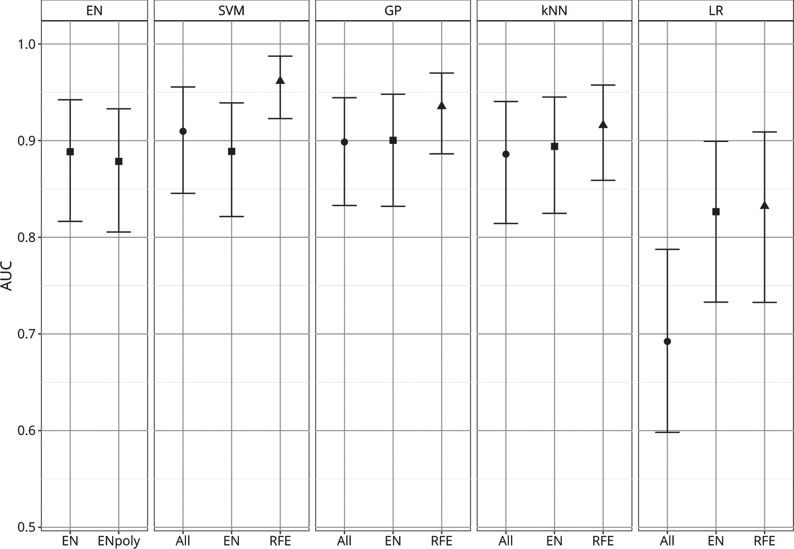
AUC of algorithms. The figure indicates the cross-validated AUC and its 95% bootstrap CI for each algorithm. Algorithms are grouped according to the machine learning techniques. The different feature selection procedure applied are indicated below, as well as by different point shapes (circle = all features; square = features selected via EN, triangle = features selected via RFE).

SVM with the features selected by the RFE procedure is the technique that achieved the highest cross-validated AUC (AUC = 0.962; C.I. 95% bootstrap = 0.923, 0.987). The results of the paired-sample t-test with stratified bootstrap resampling evidenced that the AUC of this model was statistically significantly higher (p < 0.05) than all other algorithms, except for the algorithm ranked second (SVM RFE versus GP RFE: p = 0.074). The model achieved high predictive performances also when the two subgroups were considered separately, although lower in the MCI subsample (AUC = 0.914; C.I. 95% bootstrap = 0.822, 0.975) and very high in the PreMCI subsample (AUC = 0.994; C.I. 95% bootstrap = 0.932, 1).

The cross-validated levels of specificity and balanced accuracy when sensitivity approached 0.95, 0.9, 0.85, 0.8, 0.75, as much as the sensitivity and specificity at the best achieved balanced accuracy are reported in Table 3. Considering the whole sample of both MCI and PreMCI subjects, the best achieved cross-validated balanced accuracy is 0.913 (sensitivity = 0.956, specificity = 0.871). Again, performances were still high but lower in magnitude in the MCI subsample, with a best balanced accuracy of 0.874 (sensitivity = 0.880, specificity = 0.867). Instead, preliminary results in the PreMCI subsample presented very high performances, with a best balanced accuracy of 0.980 (sensitivity = 1, specificity = 0.960).

Table 3

Performance metrics of the best model, SVM with features selected by RFE

	Sensitivity (Actual)	Specificity	Balanced Accuracy
Whole Sample (AUC = 0.962)
Sensitivity of 0.95	0.950	0.874	0.912
Sensitivity of 0.90	0.900	0.906	0.903
Sensitivity of 0.85	0.850	0.938	0.894
Sensitivity of 0.80	0.800	0.951	0.876
Sensitivity of 0.75	0.750	0.957	0.853
Best Balanced Accuracy	0.956	0.871	0.913
Only MCI (AUC = 0.914)
Sensitivity of 0.95	0.951	0.734	0.843
Sensitivity of 0.90	0.901	0.822	0.862
Sensitivity of 0.85	0.851	0.877	0.864
Sensitivity of 0.80	0.801	0.882	0.842
Sensitivity of 0.75	0.751	0.883	0.817
Best Balanced Accuracy	0.880	0.867	0.874
Only PreMCI (AUC = 0.994)
Sensitivity of 0.95	0.955	0.960	0.958
Sensitivity of 0.90	0.904	0.966	0.935
Sensitivity of 0.85	0.853	0.966	0.910
Sensitivity of 0.80	0.802	0.966	0.884
Sensitivity of 0.75	0.751	0.966	0.859
Best Balanced Accuracy	1.000	0.960	0.980

AUC, area under the receiving operating curve; MCI, mild cognitive impairment; PreMCI, premild cognitive impairment.

Efficacy of feature selection procedures

The features selected by both the EN model with the best hyper-parameter configuration and the RFE procedure are also specified in Table 1. The RFE procedure used in this study resulted effective in identifying a relevant subset of the initial features, leading in all techniques to a significant improvement of the cross-validated performances compared to the use of all features (SVM versus SVM RFE: p = 0.015; GP versus GP RFE: p = 0.023; kNN versus kNN RFE: p = 0.048; LR versus LR RFE: p < 0.001). Moreover, also the models ranked second and third were GP and kNN with the features selected by the RFE procedure and they both achieved a AUC higher than 0.9.

Instead, the approach of using the features selected by the EN model was not particularly efficacious, leading to not statistically significant improvements in GP, kNN, and LR and even leading to a reduced performance in SVM.

Feature importance

The LPOCV AUC of each of the 36 features is reported in Table 4, ranked from the highest to the lowest AUC, and in Fig. 2, subdivided based on their type (i.e., sociodemographic, diagnosis, clinical, VRS, neuropsychological tests, and of cardiovascular risk indexes).

Table 4

Feature importance

Feature	LPOCV AUC	CI 95% (Bootstrap)		Statistical Significance
Hopkins Verbal Learning Test Revised, Delayed Recall	0.812	0.722	0.887	x
Semantic Interference Test, Retroactive Total Score	0.810	0.715	0.888	x
Diagnosis	0.795	0.712	0.862	x
Logical Memory, Delayed Recall Score (WMS-IV)	0.794	0.703	0.871	x
Logical Memory, Immediate Recall Score (WMS-IV)	0.789	0.688	0.868	x
Hopkins Verbal Learning Test Revised, Total Recall	0.779	0.687	0.858	x
Semantic Interference Test, Recognition Total Score	0.778	0.664	0.868	x
Right entorhinal cortex atrophy (VRS)	0.761	0.654	0.853	x
Left hippocampus atrophy (VRS)	0.732	0.629	0.827	x
Modified Clinical Dementia Rating Scale, Memory Sum Score	0.730	0.627	0.824	x
Right hippocampus atrophy (VRS)	0.721	0.614	0.816	x
Delayed Visual Reproduction (WMS-IV)	0.718	0.599	0.818	x
Left entorhinal cortex atrophy (VRS)	0.708	0.597	0.809	x
Right perirhinal cortex atrophy (VRS)	0.691	0.585	0.794	x
Trial Making A, Time (s)	0.664	0.554	0.765	x
Trial Making B, Time (s)	0.659	0.543	0.766	x
Left perirhinal cortex atrophy (VRS)	0.647	0.538	0.753	x
History of stroke/TIA	0.630	0.580	0.686	x
Trial Making B, Errors	0.625	0.515	0.733	x
Age	0.622	0.501	0.732	x
History of coronary bypass/angioplasty	0.618	0.567	0.671	x
Body-Mass Index	0.609	0.495	0.714
Block Design Test, Raw Score (WAIS-III)	0.600	0.480	0.710
Education (y)	0.599	0.477	0.719
Digit-Symbol-Coding Score (WAIS-III)	0.596	0.478	0.706
Heart Rate (in beats-per-minute)	0.584	0.463	0.697
Hypercholesterolemia	0.566	0.472	0.649
Similarities Test, raw score (WAIS-III)	0.563	0.446	0.676
Clinical Dementia Rating Scale, Global Score	0.559	0.522	0.591	x
Hypertension	0.541	0.437	0.640
History of myocardial infarction	0.540	0.480	0.612
Trial Making A, Errors	0.526	0.454	0.581
Gender	0.520	0.416	0.619
History of tobacco use	0.516	0.461	0.548
Geriatric Depression Scale	0.512	0.409	0.615
Diabetes	0.509	0.426	0.569

WAIS-III, Wechsler Adult Intelligence Scale – Version 3; WMS-IV, Weschler Memory Scale – Fourth Edition; VRS, Visual Rating Scale; AUC, area under the receiving operating curve; LPOCV, leave-pair-out cross-validation; CI, confidence interval.

Fig.2

AUC of individual predictors. The figure indicates the cross-validated AUC and its 95% bootstrap CI when prediction is made by each single predictor. Predictors are grouped according to conceptual domains, in descending order sociodemographic information, diagnosis, clinical scores, brain atrophy, cognitive measures and cardiovascular risk index. Non-significant AUC (i.e., lower bound of the CI lower than or equal to 0.5) are in grey, significant ones in black.

The sociodemographic features had poor predictive capability. All their AUC resulted below 0.65 and only age achieved statistical significance (lower bound of the 95% C.I. higher than 0.5). As a matter of facts, neither the EN model nor the RFE procedures selected any of the sociodemographic features to be included in the models.

The baseline diagnosis (i.e., aMCI, non-aMCI, PreMCI-np, and PreMCI-cl) resulted instead quite predictive, with an AUC of 0.759. This is again in accordance with both the feature selection procedure that identified these features as those to be retained.

Among the clinical scales, only the ModCDR-M score resulted with both a significant and relevant cross-validated AUC (AUC = 0.730), being the sole selected by both the feature selection procedures. The global CDR score, although resulting with a statistically significant AUC, had an AUC very small in magnitude (AUC = 0.559).

The AUC of the six VRS scores ranged from 0.761 (right ERC atrophy) to 0.647 (the left PRC atrophy). The left PRC atrophy score was the sole not selected by the RFE procedure while all VRS scores were included in the final EN model.

Among the fourteen neuropsychological test scores, the HVLTR-R and HVLTR-D scores, the SIT-RT and SIT-RC scores, LM-I and LM-D scores of the Weschler Memory Scale – Fourth Edition (WMS-IV) resulted the tests with the highest predictive performances (all AUC above 0.750) and these were all selected by both the feature selection procedures. The DVR score of the WMS-IV also resulted able to provide statistically significant although less precise prediction of conversion (AUC = 0.718), as much as TMT-A and TMT-B errors (AUC ranging between 0.6 and 0.7). Of these, both time and errors of the TMT-B resulted included also in the final EN model, while the RFE procedure selected only TMT-B errors.

Finally, among the cardiovascular risk features, only history of stroke/TIA and history of coronary bypass/angioplasty were found to have an AUC statistically significant and higher than 0.6. Interestingly, the selection of these features by the two feature selection procedures resulted quite different from this evidence. The final EN model did not include any of the cardiovascular risk features, while the RFE selected history of myocardial infarction and heart rate, which had a non-significant LPOCV AUC, and not history of myocardial infarction and history of coronary bypass/angioplasty.

DISCUSSION

The current study represents the first step in the development of a novel machine-learning algorithm for the identification of three-year conversion to AD in subjects with either MCI or PreMCI. Such an algorithm aims in the end to be efficiently applicable in clinical practice, which require it to achieve high accuracy and to be based on predictors that can be easily and effectively assessed in clinical settings.

The algorithms developed in this study promise to fulfill both these requirements. We employed only predictors based on sociodemographic characteristics, clinical and neuropsychological tests, cardiovascular risk indexes, and level of brain atrophy as assessed by clinicians through the VRS from structural MRI images. With these pieces of information, our best algorithm achieved a global cross-validated AUC higher than 0.96, with a AUC higher than 0.91 also in the MCI subsample. This indicates that our best algorithm already outperforms the clear majority of the several previously proposed algorithms. Furthermore, to the best of our knowledge, this is the only available predictive model that was developed for subjects at a PreMCI stage, showing very high preliminary performance (AUC > 0.99) also in the PreMCI subgroup.

Translation to clinical practice

Among all the algorithms we developed, the one which showed the best performance was the SVM with radial-basis function kernel that included only the features selected via the RFE procedure. Regarding the MCI subsample, roughly 88% of specificity and 87% sensitively are the levels that resulted maximizing the overall cross-validated balanced accuracy (87%). We also found results of a nearly perfect identification of cAD in the PreMCI subsample (cross-validated accuracy = 98%), although these should be considered preliminary as we only had three cAD PreMCI subjects in our sample. Further testing in independent clinical samples would finally confirm these results.

The predictive capabilities achieved by this model would make its application useful in clinical practice as much as in clinical trials, representing a relevant improvement in the current possibility to identify only those subjects truly at risk of converting to AD. Moreover, it would be possible to further optimize the desired levels of specificity and sensitivity according to the cost associated in predicting false positives and negatives.

In addition, although the prediction scores output by some techniques does not represent true probabilities, there are procedures that can calibrate them so that they can provide the individual risk of conversion. Considering that having not only a categorical prediction but also the associated risk of conversion would be of great clinical utility, we plan to perform such calibration with Platt scaling [50] or isotonic regression in the next step of the development of the algorithm, when a further independent sample will be available.

We achieved the obtained results employing routine collectable information. All the measures we used as predictors are non-invasive and can be easily introduced in any clinical center without requiring any particular difficulty or the purchase of non-standardly available equipment. All the neuropsychological tests do not necessitate any intensive training and can be administered by a technician under the supervision of a neuropsychologist. Moreover, the availability of machines for structural MRI is now widespread and the VRS is fast and easily adoptable thanks to the availability of a software with reference images that guide the clinician during the rating, providing training for the relatively uninitiated radiologist, neurologist, or any other interested rater [34]. The VRS overcomes the issue of MRI data obtained from different machines, which are usually non-automatically comparable. All the remaining information we considered, such as socio-demographic, clinical, and cardiovascular risk, can be readily collected during neurological interviews.

Comparisons with other available machine learning algorithms

Several machine learning algorithms have been previously proposed to predict the MCI to AD conversion. Among those that used only baseline information and make a prediction of conversion in about three years, we could identify only a few achieving performances similar or superior to the ours, and they are reported in Table 5.

Table 5

Comparison with previous algorithms for MCI subjects with comparable or superior performances

Reference	Follow-up Period	Predictors	Machine Learning Technique	Validation Protocol	Sample Size	AUC	Specificity	Sensitivity	Balanced Accuracy
Our best algorithm	3 years	Socio-demographic, clinical, neuropsychological test scores, clinician-rated brain atrophy, cardiovascular risk scores	SVM with radial-basis function kernel	Leave-pair-out cross-validation	61	0.914	0.880	0.867	0.874
Plant et al. [20]	Approximately 2.5 years	Structural MRI	Linear SVM	Leave-one-out cross-validation	24	n.a.	0.889	1.000	0.945
			Bayesian Classifier	Leave-one-out cross-validation		n.a.	0.778	1.000	0.889
			Voting Feature Intervals	Leave-one-out cross-validation		n.a.	1.000	0.933	0.967
Hojjati et al. [25]	3 years	Resting-state functional MRI	Linear SVM	Repeated-9-fold cross-validation	80	0.949	0.901	0.832	0.867
Minhas et al. [19]	3 years	Structural MRI, neuropsychological test scores	Novel non-parametric approach	Leave-one-out cross-validation	13	n.a.	0.923	0.875	0.899
Agarwal et al. [18]	5/6 years	Blood plasma proteins	Radial-basis function network	Repeated 5-fold cross-validation (10 repetitions)	47	n.a.	>0.9	>0.95	>0.925
Long et al. [26]	3 years	Structural MRI	Linear SVM	10-fold cross-validation	227	0.932	0.909	0.863	0.886
Dukart et al. [23]	At least 2 years	APOE typization, FDG-PET, and structural MRI	Naïve Bayes	Train dataset: AD+controls; Test dataset: MCI	192	0.840	0.861	0.875	0.868
Moradi et al. [22]	3 years	Structural MRI, neuropsychological test scores and age	Semi-supervised approach and Random Forest	10-fold cross-validation	264	0.902	0.740	0.870	0.805
Apostolova et al. [24] (only ApoE4-negative subjects)	3 years	Cerebrospinal fluid p-tau, education, sex	SVM with radial-basis function kernel	Leave-one-out cross-validation	83	0.890	n.a.	n.a.	n.a.
Clark et al. [21]	At least 1 year	Socio-demographic, clinical, and neuropsychological test scores	Random Forest	10-fold cross-validation	80	0.880	0.890	0.770	0.840
Clark et al. [52]	>4 years	Socio-demographic, clinical, and neuropsychological test scores	Ensemble of Random Forest, SVM, Naïve Bayes, and Multi-Layer Perceptron	Leave-one-out cross-validation	107	0.872	0.880	0.708	0.794
Johnson et al. [53]	3 years	Clinical, and neuropsychological test scores	Logistic Regression	Repeated 5-fold cross-validation (5 repetitions)	77	0.870	n.a.	n.a.	n.a.

AUC, area under the receiving operating curve; SVM, support vector machine.

Specifically, five studies evidenced superior performances. The algorithm proposed by Argwal and colleagues [18] uses a selection of blood plasma proteins as sole predictors. This is a very interesting result as their model uses information from a different domain and it may be partially complementary to the features we used. Also, the prediction is entirely based on the analysis of a single blood sample and even if the assessment of such protein blood levels is not currently clinical routine, it requires a very little invasive procedure and may be developed so to result cost-effectively adoptable in clinical practice. However, these results come from a small training sample and further investigation is necessary to evidence the soundness of such promising results.

Three further algorithms have been developed based on structural MRI data: those proposed by Minhas and colleagues [19], and Plant and colleagues [20] were trained and cross-validated in very small samples, respectively of 13 and 24 MCI subjects, while Long and colleagues [26] used a larger sample (n = 227). All these algorithms showed very high cross-validated performance. However, they directly use structural MRI data and considering the difficulties of employing together data coming from different scanners [51], this may place a barrier to an efficient dissemination of such algorithms into clinical practice.

Finally, also Hojjati and colleagues proposed an algorithm [25] with high predictive accuracy based on resting state functional MRI data. If the availability of MRI machines in clinical setting is quite common nowadays, functional MRI is still mainly used in research settings. Thus, such algorithm may currently result difficulty applicable in clinical practice.

Additional studies proposed algorithm with performances similar to the ours. Three studies employed predictors that may not allow an easy translation to clinical practice: Morandi and colleagues [22] used structural MRI data, Dukart and colleagues [23] both structural MRI and fludeoxyglucose positron emission tomography data, and Apostolova and colleagues [24] cerebrospinal fluid p-tau protein levels.

Instead, Clark and colleagues [21] used only sociodemographic, clinical, and neuropsychological test scores, achieving high cross-validated performances although inferior to those achieved by our best model. Two other studies proposed algorithms based only on these types of predictive information [52, 53]. They also achieved high predictive performances but inferior to Clark’s algorithm.

Considering this evidence, our and these three algorithms are the only currently available that achieved a relevant predictive performance using only predictors that may be easily assessed in nowadays clinical practice, with our algorithm that seems to outperform all of them. As we used different predictors than those employed in these other algorithms (i.e., they did not use brain atrophy levels assessed via the VRS but included the scores of different neuropsychological tests), it would be of great interest to investigate in the next steps if adding such predictors to our features would bring a further increase in the predictive performance of our algorithm.

Importance of predictors

As mentioned above, the interpretation of the predictor importance in non-linear models, such as SVM, GP, and kNN, is a complex and not yet solved issues. Considering this, in the current study we decided to focus only on evaluating the individual importance of each 36 predictors initially considered in this study.

While sociodemographic and cardiovascular risk were not particularly predictive, memory and brain atrophy seems to be the most relevant for the prediction of AD conversion. The HVLTR, SIT, and LM tests were identified as the most relevant cognitive measures by all feature selection and importance procedures and they all assess different aspects of memory. The ModCDR-M score was also suggested as a particularly relevant feature. The important role of memory functioning as predictor was somehow expected considering previous findings [54] and that memory deficits are the core clinical characteristics that defines AD. Also, the evidence of an important role of brain atrophy is in line with previous evidence [55] as well as several other studies which developed highly performing machine learning algorithms starting from structural MRI data, alone (i.e., [20]) or in combination with neuropsychological test scores (i.e., [19, 22]). Memory deterioration and brain atrophy may begin years before a full-blown AD diagnosis can be made and a proper set of sensible measures can allow to promptly identify them. Our study further suggests that machine learning techniques have the potential to exploit such information to early identify those subjects in which the onset of the pathophysiological processes leading to AD has been occurring.

Limitations

Our study has some potential limitations that should be taken into account. We used cross-validation as validation procedure but further testing in an independent sample of new cases has not been performed yet. However, nearly all the algorithms proposed to make a MCI-to-AD prediction currently lack such further testing. Furthermore, the sample we used to train the algorithm was limited in size and included only three cAD PreMCI. Thus, the performance estimate obtained for the PreMCI should be considered as very preliminary and requires further investigation.

We applied only some of the many machine learning as well as feature selection procedures available. Although we have already reached good results, there is no guarantee that other machine learning procedures and other subsets of features would allow to achieve even better predictive accuracy.

Moreover, all subjects of our sample were recruited in the same abovementioned clinical centers. The population referring to these might have peculiar characteristics and algorithms might perform less well in different MCI and PreMCI populations. Also, both the features and subjects we finally included were selected from a larger set of available variables and subjects according to the lack of missing values. Their occurrence in such excluded variables and subjects may be due to reasons that are beyond mere randomness, potentially limiting the representativeness of our feature set and train sample and thus leading to biases in our algorithm.

Given these current issues, we plan to test the performance in a new sample of MCI and PreMCI subjects participating in a new longitudinal study in Miami, currently in its third year, as well as to try new procedures for further optimization.

Another potential shortcoming is the complexity of providing a clear explanation of the role that each feature plays in the prediction. While a first basic approach has been attempted in this study, more strategies will be applied while proceeding in the next phases with larger samples and a future study will be addressed in attempting to open the model black-box. A better interpretability of the model will help both in gaining further understandings of how these variables are related to the development of AD and in generating more trust towards the application of model by clinicians as much as patients.

Conclusion

In conclusion, we used supervised machine learning techniques to develop algorithms able to identify which subjects with PreMCI and MCI will convert to AD in the following three years. As the opportunity of an efficient clinical translation was one of the main goal motivating our study, we used predictors based only on sociodemographic characteristics, clinical tests, cognitive measures, cardiovascular risk indexes, and level of brain atrophy as assessed by clinicians through the VRS from structural MRI images. We promisingly achieved high predictive performance, among the very best of the many algorithms available in literature and the best achieved so far using only information easily collectable in clinical practice. Considering these results, we plan to proceed in further testing and optimization in other independent and larger samples as to reach the level of reliability necessary for an actual applicability.

Footnotes

ACKNOWLEDGMENTS

This study was supported by the National Institute on Aging, United States Department of Health and Human Services (grant: 1P50AG025711-05, R01AG047649-01A1, P50 AG047726602).

Authors’ disclosures available online ().

References

Alzheimer Disease International (2016), World Alzheimer Report 2016. Improving healthcare for people living with dementia. London.

Szeto

, Lewis

(2016) Current treatment options for Alzheimer’s disease and Parkinson’s disease dementia. Curr Neuropharmacol 14, 326–338.

Brooks

, Loewenstein

(2010) Assessing the progression of mild cognitive impairment to Alzheimer’s disease: Current trends and future directions. Alzheimers Res Ther 2, 28.

Loewenstein

, Curiel

, Duara

, Buschke

(2017) Novel cognitive paradigms for the detection of memory impairment in preclinical Alzheimer’s disease. Assessment, 1073191117691608.

Petersen

, Parisi

, Dickson

, Johnson

, Knopman

, Boeve

, Jicha

, Ivnik

, Smith

, Tangalos

, Braak

, Kokmen

(2006) Neuropathologic features of amnestic mild cognitive impairment. Arch Neurol 63, 665–672.

Roberts

, Knopman

, Mielke

, Cha

, Pankratz

, Christianson

, Geda

, Boeve

, Ivnik

, Tangalos

, Rocca

, Petersen

(2014) Higher risk of progression to dementia in mild cognitive impairment cases who revert to normal. Neurology 82, 317–325.

Chao

, Mueller

, Buckley

, Peek

, Raptentsetseng

, Elman

, Yaffe

, Miller

, Kramer

, Madison

, Mungas

, Schuff

, Weiner

(2010) Evidence of neurodegeneration in brains of older adults who do not yet fulfill MCI criteria. Neurobiol Aging 31, 368–377.

Loewenstein

, Greig

, Schinka

, Barker

, Shen

, Potter

, Raj

, Brooks

, Varon

, Schoenberg

, Banko

, Potter

, Duara

(2012) An investigation of PreMCI: Subtypes and longitudinal outcomes. Alzheimers Dement 8, 172–179.

Breitner

(2014) Mild cognitive impairment and progression to dementia: New findings. Neurology 82, e34–35.

10.

Forlenza

, Diniz

, Teixeira

, Stella

, Gattaz

(2013) Mild cognitive impairment. Part 2: Biological markers for diagnosis and prediction of dementia in Alzheimer’s disease. Rev Bras Psiquiatr 35, 284–294.

11.

Sperling

, Johnson

(2013) Biomarkers of Alzheimer disease: Current and future applications to diagnostic criteria. Continuum (Minneap Minn) 19, 325–338.

12.

van Rossum

, Vos

, Handels

, Visser

(2010) Biomarkers as predictors for conversion from mild cognitive impairment to Alzheimer-type dementia: Implications for trial design. J Alzheimers Dis 20, 881–891.

13.

Kang

, Korecka

, Toledo

, Trojanowski

, Shaw

(2013) Clinical utility and analytical challenges in measurement of cerebrospinal fluid amyloid-beta(1-42) and tau proteins as Alzheimer disease biomarkers. Clin Chem 59, 903–916.

14.

Cooper

, Sommerlad

, Lyketsos

, Livingston

(2015) Modifiable predictors of dementia in mild cognitive impairment: A systematic review and meta-analysis. Am J Psychiatry 172, 323–334.

15.

Van Cauwenberghe

, Van Broeckhoven

, Sleegers

(2016) The genetic landscape of Alzheimer disease: Clinical implications and perspectives. Genet Med 18, 421–430.

16.

Klunk

(2011) Amyloid imaging as a biomarker for cerebral beta-amyloidosis and risk prediction for Alzheimer dementia.S. Neurobiol Aging 32(Suppl 1), 20–36.

17.

Samuel

(1959) Some studies in machine learning using the game of checkers. IBM J Res Dev 3, 210–229.

18.

Agarwal

, Ghanty

, Pal

(2015) Identification of a small set of plasma signalling proteins using neural network for prediction of Alzheimer’s disease. Bioinformatics 31, 2505–2513.

19.

Minhas

, Khanum

, Riaz

, Alvi

, Khan

(2017) A nonparametric approach for mild cognitive impairment to AD conversion prediction: Results on longitudinal data. IEEE J Biomed Health Inform 21, 1403–1410.

20.

Plant

, Teipel

, Oswald

, Bohm

, Meindl

, Mourao-Miranda

, Bokde

, Hampel

, Ewers

(2010) Automated detection of brain atrophy patterns based on MRI for the prediction of Alzheimer’s disease. Neuroimage 50, 162–174.

21.

Clark

, Kapur

, Geldmacher

, Brockington

, Harrell

, DeRamus

, Blanton

, Lokken

, Nicholas

, Marson

(2014) Latent information in fluency lists predicts functional decline in persons at risk for Alzheimer disease. Cortex 55, 202–218.

22.

Moradi

, Pepe

, Gaser

, Huttunen

, Tohka

, Alzheimer’s Disease Neuroimaging Initiative (2015) Machine learning framework for early MRI-based Alzheimer’s conversion prediction in MCI subjects. Neuroimage 104, 398–412.

23.

Dukart

, Sambataro

, Bertolino

(2016) Accurate prediction of conversion to Alzheimer’s disease using imaging, genetic, and neuropsychological biomarkers. J Alzheimers Dis 49, 1143–1159.

24.

Apostolova

, Hwang

, Kohannim

, Avila

, Elashoff

, Jack

Jr , Shaw

, Trojanowski

, Weiner

, Thompson

, Alzheimer’s Disease Neuroimaging Initiative (2014) ApoE4 effects on automated diagnostic classifiers for mild cognitive impairment and Alzheimer’s disease. Neuroimage Clin 4, 461–472.

25.

Hojjati

, Ebrahimzadeh

, Khazaee

, Babajani-Feremi

, Alzheimer’s Disease Neuroimaging Initiative (2017) Predicting conversion from MCI to AD using resting-state fMRI, graph theoretical approach and SVM. J Neurosci Methods 282, 69–80.

26.

Long

, Chen

, Jiang

, Zhang

, Alzheimer’s Disease Neuroimaging Initiative (2017) Prediction and classification of Alzheimer disease based on quantification of MRI deformation. PLoS One 12, e0173372.

27.

American Psychiatric Association (2000) Diagnostic and Statistical Manual of Mental Disorders DSM-IV-TR Fourth Edition (Text Revision). American Psychiatric Association, Washington, DC.

28.

McKhann

, Drachman

, Folstein

, Katzman

, Price

, Stadlan

(1984) Clinical diagnosis of Alzheimer’s disease: Report of the NINCDS-ADRDA Work Group under the auspices of Department of Health and Human Services Task Force on Alzheimer’s Disease. Neurology 34, 939–944.

29.

Duara

, Loewenstein

, Potter

, Appel

, Greig

, Urs

, Shen

, Raj

, Small

, Barker

, Schofield

, Wu

, Potter

(2008) Medial temporal lobe atrophy on MRI scans and the diagnosis of Alzheimer disease. Neurology 71, 1986–1992.

30.

Morris

(1993) The Clinical Dementia Rating (CDR): Current version and scoring rules. Neurology 43, 2412–2414.

31.

Duara

, Loewenstein

, Greig-Custo

, Raj

, Barker

, Potter

, Schofield

, Small

, Schinka

, Wu

, Potter

(2010) Diagnosis and staging of mild cognitive impairment, using a modification of the clinical dementia rating scale: The mCDR. Int J Geriatr Psychiatry 25, 282–289.

32.

Sheikh

, Yesavage

(1986) Geriatric Depression Scale (GDS): Recent evidence and development of a shorter version. In Clinical Gerontology: A Guide to Assessment and Interventions. The Haworth Press, NY, pp. 165–173.

33.

Scheltens

, Leys

, Barkhof

, Huglo

, Weinstein

, Vermersch

, Kuiper

, Steinling

, Wolters

, Valk

(1992) Atrophy of medial temporal lobes on MRI in “probable” Alzheimer’s disease and normal ageing: Diagnostic value and neuropsychological correlates. J Neurol Neurosurg Psychiatry 55, 967–972.

34.

Urs

, Potter

, Barker

, Appel

, Loewenstein

, Zhao

, Duara

(2009) Visual rating system for assessing magnetic resonance images: A tool in the diagnosis of mild cognitive impairment and Alzheimer disease. J Comput Assist Tomogr 33, 73–78.

35.

Varon

, Barker

, Loewenstein

, Greig

, Bohorquez

, Santos

, Shen

, Harper

, Vallejo-Luces

, Duara

, Alzheimer’s Disease Neuroimaging Initiative (2015) Visual rating and volumetric measurement of medial temporal atrophy in the Alzheimer’s Disease Neuroimaging Initiative (ADNI) cohort: Baseline diagnosis and the prediction of MCI outcome. Int J Geriatr Psychiatry 30, 192–200.

36.

Benedict

, Zgaljardic

(1998) Practice effects during repeated administrations of memory tests with and without alternate forms. J Clin Exp Neuropsychol 20, 339–352.

37.

Loewenstein

, Acevedo

, Luis

, Crum

, Barker

, Duara

(2004) Semantic interference deficits and the detection of mild Alzheimer’s disease and mild cognitive impairment without dementia. J Int Neuropsychol Soc 10, 91–100.

38.

Reitan

(1958) Validity of the Trail Making Test as an indicator of organic brain damage. Percept Mot Skills 8, 271–276.

39.

Wechsler

(1997) WAIS-III: Administration and scoring manual: Wechsler adult intelligence scale, Psychological Corporation.

40.

Wechsler

(1997) WMS-III: Wechsler memory scale administration and scoring manual, Psychological Corporation.

41.

Zou

, Hastie

(2005) Regularization and variable selection via the Elastic Net. J R Stat Soc Series B Stat Methodol 67, 301–320.

42.

Schölkopf

, Smola

(2002), Learning with kernels: Support vector machines, regularization, optimization, and beyond, MIT press.

43.

Rasmussen

(2006) Gaussian processes for machine learning, The MIT Press, Cambridge.

44.

Core Team

(2017), R Foundation for Statistical Computing.

45.

Kuhn

(2008) Building predictive models in R using the caret package. J Stat Softw 28.

46.

Airola

, Pahikkala

, Waegeman

, De Baets

, Salakoski

(2011) An experimental comparison of cross-validation techniques for estimating the area under the ROC curve. Comput Stat Data Anal 55, 1828–1844.

47.

Parker

, Gunter

, Bedo

(2007) Stratification bias in low signal microarray studies. BMC Bioinformatics 8, 326.

48.

Efron

(1987) Better bootstrap confidence intervals. J Am Stat Assoc 82, 171–185.

49.

Carpenter

, Bithell

(2000) Bootstrap confidence intervals: When, which, what? A practical guide for medical statisticians. Stat Med 19, 1141–1164.

50.

Platt

(1999) Probabilistic outputs for support vector machines and comparisons to regularized likelihood methods. Adv Large Margin Classifiers 10, 61–74.

51.

Teipel

, Reuter

, Stieltjes

, Acosta-Cabronero

, Ernemann

, Fellgiebel

, Filippi

, Frisoni

, Hentschel

, Jessen

, Kloppel

, Meindl

, Pouwels

, Hauenstein

, Hampel

(2011) Multicenter stability of diffusion tensor imaging measures: A European clinical and physical phantom study. Psychiatry Res 194, 363–371.

52.

Clark

, McLaughlinc

, Wood

, Hwange

, Hurtzf

, Ramirezf

, Eastmang

, Dukesa

, Kapurh

, DeRamusi

, Apostolovaj

(2016) Novel verbal fluency scores and structural brain imaging for prediction of cognitive outcome in mild cognitive impairment. Alzheimers Dement (Amst) 2, 113–122.

53.

Johnson

, Vandewater

, Wilson

, Maruff

, Savage

, Graham

, Macaulay

, Ellis

, Szoeke

, Martins

, Rowe

, Masters

, Ames

, Zhang

(2014) Genetic algorithm with logistic regression for prediction of progression to Alzheimer’s disease. BMC Bioinformatics 15 Supp 16, S11.

54.

Loewenstein

, Acevedo

, Agron

, Duara

(2007) Vulnerability to proactive semantic interference and progression to dementia among older adults with mild cognitive impairment. Dement Geriatr Cogn Disord 24, 363–368.

55.

, Tan

, Wang

, Tan

, Xu

, Zhao

, Wang

, Jiang

, Yu

(2016) Risk factors for predicting progression from mild cognitive impairment to Alzheimer’s disease: A systematic review and meta-analysis of cohort studies. J Neurol Neurosurg Psychiatry 87, 476–484.