Screening for Alzheimer’s Disease Using Saliva: A New Approach Based on Machine Learning and Raman Hyperspectroscopy

Abstract

Background:

Alzheimer’s disease and related dementias (ADRDs) are being diagnosed at epidemic rates, with incidence to triple from 35 to 115 million cases worldwide. Most ADRDs are characterized by progressive neurodegeneration, and Alzheimer’s disease (AD) is the sixth leading cause of death in the United States. The ideal moment for diagnosing ADRDs is during the earliest stages of its progression; however, current diagnostic methods are inefficient, expensive, and unsuccessful at making diagnoses during the earliest stages of the disease.

Objective:

The aim of this project was to utilize Raman hyperspectroscopy in combination with machine learning to develop a novel method for the diagnosis of AD based on the analysis of saliva.

Methods:

Raman hyperspectroscopy was used to analyze saliva samples collected from normative, AD, and mild cognitive impairment (MCI) individuals. Genetic Algorithm and Artificial Neural Networks machine learning techniques were applied to the spectral dataset to build a diagnostic algorithm.

Results:

Internal cross-validation showed 99% accuracy for differentiating the three classes; blind external validation was conducted using an independent dataset to further verify the results, achieving 100% accuracy.

Conclusion:

Raman hyperspectroscopic analysis of saliva has a remarkable potential for use as a non-invasive, efficient, and accurate method for diagnosing AD.

Keywords

Alzheimer’s disease artificial neural networks early diagnosis genetic algorithm machine learning mild cognitive impairment Raman spectroscopy saliva

INTRODUCTION

Alzheimer’s disease (AD) is the most common form of neurodegeneration-induced dementia in the elderly population worldwide [1]. In the United States alone, an estimated 5.7 million Americans are affected by the disease, which is also the sixth leading cause of death [2]. The rapid increase in number of AD patients, combined with overall increased life expectancy and lack of effective treatment, has had a devastating impact on healthcare systems in industrialized nations across the world. In fact, in 2018 alone, the disease cost the United States almost $300 billion [2]. Its devastating impact has worsened due to the fact that AD is progressive, incurable, and lethal.

The etiology and pathogenesis of AD are highly complex, and several major factors have been found to play an important role in its progression. The most prominent theory says the disease is caused by the build-up of the amyloid-β (Aβ) protein within the brain, which then forms the typical plaques and neurofibrillary tangles that are characteristic of the disease [3]. Hyper-phosphorylation of the tau protein is also believed to play an imperative role in causing the neurodegeneration associated with AD [4]. While the complete causation of the disease remains questioned, it is believed that the disease begins years before clinical manifestations arise [5, 6].

The lack of a complete set of information surrounding what causes AD deters the development of simple diagnostic methods. In fact, there is no single test currently capable of diagnosing AD that is approved for use in clinical settings or at the point of care [2]. A combination of many different tests and exams is usually conducted in order to aid in making a diagnosis, including a complete medical exam, mental status tests, neurological exams, and brain imaging tests. The combination of these tests is time consuming, expensive, and can be invasive, especially for repetitive use in older adults. Ideally, a definitive method for diagnosing the disease early on in its progression, before neurodegeneration becomes too severe, is desired; this will allow for initiation of disease-modifying treatments at the earliest stages of AD [7].

The development of a new noninvasive diagnostic method based on body fluid analysis that integrates multiple biomarkers can significantly improve the accuracy of diagnosis. Recent studies analyzing blood, saliva, and cerebrospinal fluid have been conducted in efforts toward developing a method for diagnosing AD [8 –13]. Of these biological materials, collection of saliva is the least invasive. Saliva is produced by several glands in the mouth, including the salivary glands [14]. It is mainly composed of water; however, the chemical components that are present in the next highest concentrations comprise of electrolytes (including bicarbonate and phosphate), mucus, various enzymes (including lipase, amylase, and lysozyme), and antibacterial compounds (including thiocyanate) [15 –17]. Saliva has been shown to have great diagnostic potential [18]. Because saliva collection is inexpensive and non-invasive, it is an attractive option for use in diagnostics. Development of a method for diagnosing AD using saliva will not only help in identifying the disease early-on for treatment intervention, but will also allow repeat analyses to be conducted in order to monitor the brain health of adults as they age. Such a widely applicable test would provide the basis for further understanding of disease-linked salivary changes, and would reduce the need for alternative, expensive, and time-consuming diagnostic methods. Moreover, a fast and reliable diagnostic test would accelerate both AD diagnosis and prognosis evaluation and would foster expedited treatment interventions.

In this regard, Raman spectroscopy has been evaluated for its diagnostic potential [19, 20]. In fact, Raman spectroscopy has been used in several applications including for diagnosing cancers, [21] asthma, [22] cornea infection, [23] and osteoarthritis [24]. Several studies have already displayed the potential of Raman spectroscopy to be used for diagnosing AD and other forms of dementia based on blood analysis [9 , 25–28]. Furthermore, Raman hyperspectroscopy is advantageous over other techniques used for disease diagnostics due to its ability to produce a spectral “fingerprint” representing the total biochemical composition of the sample and, as such, combining the contribution from several biochemical markers of the disease. Because of this, Raman hyperspectroscopy has the potential to detect changes occurring in biological samples during the onset and progression of a disease.

This proof-of-concept study focused on understanding the selectivity of Raman hyperspectroscopy in combination with machine learning through the examination of Raman spectral profiles of saliva collected from normative, AD, or mild cognitive impairment (MCI) individuals. Machine learning, sometimes referred to as multivariate statistical methods, were used to generate a classification model that capitalizes on differences between spectral profiles of the three classes, which then was used to diagnose a person with AD or with MCI with high levels of accuracy. Specifically, Artificial Neural Networks (ANN) was used. Furthermore, it was found that feature selection could benefit multivariate analysis by removing irrelevant or redundant variables from a dataset. Thus, Genetic Algorithm (GA) was used as the feature selection technique; the combination of GA with ANN improved the classification model’s performance by achieving deeper understanding of what spectral variables were important as well as by simplifying the model through elimination of irrelevant features of the data set. Ideally, GA should select features in the Raman spectra of saliva that are associated with neurodegeneration-induced dementia. A diagnostic ANN model was built with the purpose of differentiating AD and MCI Raman spectra from spectra of normative donors, and was optimized based on GA-selected spectral features. This novel concept delivers a crucial step toward creating a simple, non-invasive, and accurate method for diagnosing AD.

MATERIALS AND METHODS

Sample collection and preparation

The 39 participants from whom saliva was collected in this study were volunteers selected from the local community; individuals were screened using a battery of neuropsychological assessments to evaluate executive function and overall cognition. The Montreal Cognitive Assessment (MoCA) and Alzheimer’s Disease Assessment Scale (ADAS) Wordlists were used as experimental diagnostic tools to differentiate between MCI, AD, and healthy age- and gender-matched controls. Information regarding the MoCA classification system can be found in Supplementary Material 1.

Participants were asked to refrain from drinking alcohol within 12 h of saliva collection; eating a major meal or brushing teeth within 1 h of collection; and eating dairy products, acidic, or high sugar-content foods, or chew on gum or candy within 30 min of collection. Any currently used medications as well as recent dental work was recorded at the time of collection. Roughly 2 mL of saliva was accumulated from each participant. The samples were then stored at -80°C.

For preparation, samples were thawed and saliva was pipetted into microfuge tubes and centrifuged for 10 min at 10,000 rpm. The supernatant was saved and used. Samples were stored at –20°C from the time of preparation to the time of analysis. For analysis, samples were thawed and 10μL of saliva was deposited on a glass microscope slide covered in aluminum foil and allowed to dry completely overnight. The aluminum foil was used as a substrate for decreasing contribution of fluorescence.

Raman spectroscopic methods

Raman spectra were collected using a Renishaw inVia Raman spectrometer equipped with a research-grade Leica microscope. The 50x objective was used to focus on the sample. All measurements were performed through use of a PRIOR automatic mapping stage. Spectra were recorded in the spectral range of 400–1700 cm^–1 under excitation by a 785 nm wavelength diode laser using WiRE 3.2 software. Laser power was reduced to 55 mW to avoid photo-degradation of the sample. The automatic mapping stage collected approximately 40 spectra per sample, with one 30-s accumulation taken at each sample position. Collecting multiple spectra per sample ensures accurate representation of the heterogeneous composition of a sample.

Data treatment

A total of 1,580 spectra from 39 total donors were imported to MATLAB (R2017b) software (Mathworks, Inc.). Any Raman spectra that showed a poor signal-to-noise ratio or cosmic rays were removed from the dataset. Four samples (donors) were randomly selected to create a holdout data set and were set aside to be used for designing an external validation experiment for independent testing of the model. These samples were only measured after the model training was finished. All spectra from the remaining 35 donors were subjected to preprocessing steps, including smoothing by automatic-weighted least squares and normalization by total area. The four samples (donors) that were set aside to create an independent, external validation dataset were preprocessed in the same manner but separately from the other data, and after the prediction model was already built. The spectral data of the 35 donors were used for variable selection and for building the classification model. GA was used to select important features to be included in the training of ANN models. The ANN analysis was performed using R-project software, ver. 3.4.3, with the “neuralnet” package [29]. Further information describing GA and ANN can be found in Supplementary Material 2.

RESULTS

Raman spectra were collected from saliva of 39 donors through the use of automatic mapping. Mapping is conducted in order to obtain multiple spectra from each sample, thereby acquiring an accurate representation of inherit compositional heterogeneity. The donors consisted of individuals from three different classes: normative (10), AD (11), and mild cognitive impairment (18) individuals. Four of the donors were separated from the rest of the samples at the beginning of the experiment, before spectral data collection and statistical analysis. After the data from the other 35 donors were processed and the final ANN model was built, the spectral data from these four samples (donors) were collected, preprocessed, analyzed and their class was predicted. The mean preprocessed spectra of each class is shown in Fig. 1A. As expected, the spectra depict the characteristic biochemical composition of saliva. The difference between the average AD and average normative spectra are depicted in Fig. 1B (additional difference spectra seen in Supplementary Material 3). The difference spectrum is shown as lying within±2 standard deviations, suggesting that the mean difference between classes is statistically insignificant, and multivariate analysis is required to uncover useful variability within individual spectra for the purpose of building diagnostic algorithms. This is not an unexpected result as the averaging of complex sets of data will result in small differences which exist within donors of a class or between classes to become hidden. As such, GA and ANN machine learning techniques were used to analyze the collected spectral data.

Fig.1

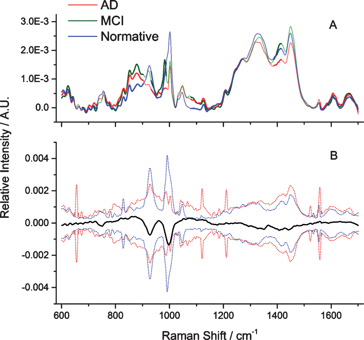
A) Pre-processed mean saliva spectra of the three classes, including the spectral ranges selected by Genetic Algorithm: AD (red), MCI (green), and normative (blue). Areas selected by Genetic Algorithm are marked as bold lines, whereas excluded spectral ranges are marked as unfilled transparent lines. B) The pre-processed difference mean saliva spectra between AD and normative (bold line) with the positive and negative 2 standard deviations (dotted lines) of the AD (red) and normative (blue) donors’ spectral data sets.

Since a large number of input variables can lead to overfitting of the ANN, and because portions of the Raman spectra are non-informative, GA was applied to reduce the variables that will be examined by the ANN classifier. GA was used to select the most informative features in the training data set consisting of 35 donors and 1440 spectra. The parameters of GA are given as follows: the population size was set to 62, the mutation rate to 0.005, and the maximum number of generations for every run was set to 100. The breeding was set to double crossover, the window width was 30 variables, and 30% of the windows were initially included. In order to pick out diagnostic feature information from the measured Raman spectra, GA was independently run 200 times, to select significant spectral bands.

The subsets of data identified by GA signify the areas of the spectra that have the strongest distinguishing capabilities between the different classes. As seen in Fig. 1, not all regions which exhibit the greatest differences between mean spectra were selected by GA; this is most likely due to the large standard deviations observed for those regions. GA iteratively split and analyzed all combinations of various subsets of spectral data with the goal of differentiating the three classes; the spectral features identified as having the lowest prediction errors “survived” and were passed along to the next potential solution. The regions and bands recognized by GA are represented by the bold lines in the spectra, as seen in Fig. 1A. The transparent lines indicate areas of the spectra that were not considered significant for differentiation purposes.

The ANN approach was used with a multilayer perceptron neural network as a classification technique and with the resilient backpropagation learning algorithm. In multivariate statistics, ANN conducts information processing in a manner that is similar to the way the human brain works. ANNs are composed of several layers of simple interconnected processing elements (i.e., neurons), which each perform a mathematical operation on input values and transfer the result to one or more hidden layers, or an output layer. The GA-identified dataset is introduced to the model through the input layer; one or more hidden layers perform processing through a system of weighted connections that perform calculations on the input data, and the output layer finally gives the classification result. Because ANN is a supervised statistical method, each donor will have a class (AD, MCI, or normative) assigned to each of its individual spectra.

During the training phase, the neural network learns the relationship between independent and dependent variables. Specifically, it learns to make associations between intensity values at specific wavelengths of the input spectral data with sample class membership, which are the designated outputs of the neural network. A total of 1,440 labeled spectra were presented to the network. During the learning phase, the network weights were adjusted to minimize differences between the output of the network and the known class labels of the samples. The process of weight optimization was based on the resilient backpropagation algorithm with weight backtracking, with a threshold set to 0.01 for defining the partial derivatives of the error function [30]. The backpropagation learning algorithm is a common method used to update weights in feedforward ANNs due to its computational efficiency [31]. Once the network weights, together with network architecture, were adjusted using the spectral dataset, the network was used to predict the labels of the unknown samples in the independent validation set. The goal was to produce a neural network model that fit the data set well while still allowing for accurate prediction of data that was not used to build the model. ANN models can be over-trained, which means they do not show good generalization due to the model fitting noise; thus, applying noise reduction techniques, such as GA, to the input data before the initiation of training can prevent overtraining of the model.

The architecture and main neural network parameters for differentiating the three classes was identified by a trial-and-error process. The network weights were trained with different configurations of the adjustable parameters and various network architectures. The performance of each ANN was assessed using the bootstrapped Latin partition (BLP) validation procedure in order to determine the optimal ANN that can differentiate AD, MCI, and normative spectra. BLP provides an unbiased evaluation of pattern recognition models. BLP divides the dataset into training and validation sets; here, nine training-validation subsets of complete samples (donors) were furnished, ensuring that each sample was only used once for prediction. The proportions of each class distribution remains fixed to maintain equal class distributions. Multiple neural network structures were built and tested using BLP to determine which structure had the best prediction capabilities.

The neural network structure that yielded the best results through validation by BLP consisted of two hidden layers, the first with 100 neurons and the second with 20 neurons. The output layer contained three neurons and was responsible for giving the predicted class. This network structure provided the lowest prediction errors for validation datasets as compared to the other networks tested in the trial-by-error process. The final network results are depicted in Table 1. Here, the performance parameters for each class, determined through BLP, are shown. The sensitivity (true-positive rate), specificity (true-negative rate), and accuracy (percentage of correctly predicted spectra among total cases) for each class prediction is reported together with 95% confidence intervals. All three classes were successfully differentiated with an average sensitivity of 98.56%, specificity of 99.29%, and accuracy of 99.14%.

Table 1

Performance parameters of the Artificial Neural Network determined using BLP

Class	Performance parameter	Value	95% Confidence interval
AD	Sensitivity	0.9887	(0.9797–0.9978)
	Specificity	0.9954	(0.9908–0.9999)
	Accuracy	0.9933	(0.9879–0.9986)
MCI	Sensitivity	0.9829	(0.9722–0.9937)
	Specificity	0.9889	(0.9826–0.9953)
	Accuracy	0.9877	(0.9813–0.9941)
Normative	Sensitivity	0.9853	(0.9754–0.9952)
	Specificity	0.9944	(0.9898–0.9981)
	Accuracy	0.9933	(0.9895–0.9971)

To verify the success of the model, “blind” external validation was conducted. Here, a total of 140 spectra from the four samples, which were previously set aside, were introduced into the validated model. To guarantee independence, spectral data was used from samples that were specifically not used in the model-building process and were only collected and preprocessed after the model training was finished. Furthermore, the classification of these samples was not known to the researcher conducting the external validation and were thus considered “blind”. Once again, the ANN model computes the probability of each individual spectrum for belonging to each class. All unlabeled spectra are then assigned to the class with the highest probability. The classification of each individual spectrum from each of the four samples is depicted in Table 2 (left-hand side), demonstrating an overall average accuracy of 72% for all three classes.

Table 2

Classification predictions for all individual spectra collected from each of the four samples (left) and overall donor-level classification predictions of the four samples (right) used for “blind” external validation

Individual spectral predictions				External validation results
Sample	Predicted class			Sample	Predicted class	True class
	AD	MCI	Normative
#1	20	8	6	#1	AD	AD
#2	5	13	14	#2	Normative	Normative
#3	18	2	14	#3	AD	AD
#4	10	30	0	#4	MCI	MCI

The overall donor-level classification of each of the four donors, based on spectral-level predictions, is shown on the right-hand side of Table 2. A donor sample was assigned to the class (MCI, AD, or normative) that received the majority of spectra assigned to it. Figure 2 plots the spectral level classifications for the four unknown samples as a percentage of spectra classified to each class, which is expressed as the height of the bar. The lowest maximum percentage was observed for Donor #2 who was assigned to the normative class with 44% of spectra correctly assigned. True classification of the samples was only revealed after the model had made its predictions. All four samples that were introduced into the model for external prediction were correctly classified. This indicates that the ANN model optimized using BLP is robust enough to reliably classify “unseen”, or new, data.

Fig.2

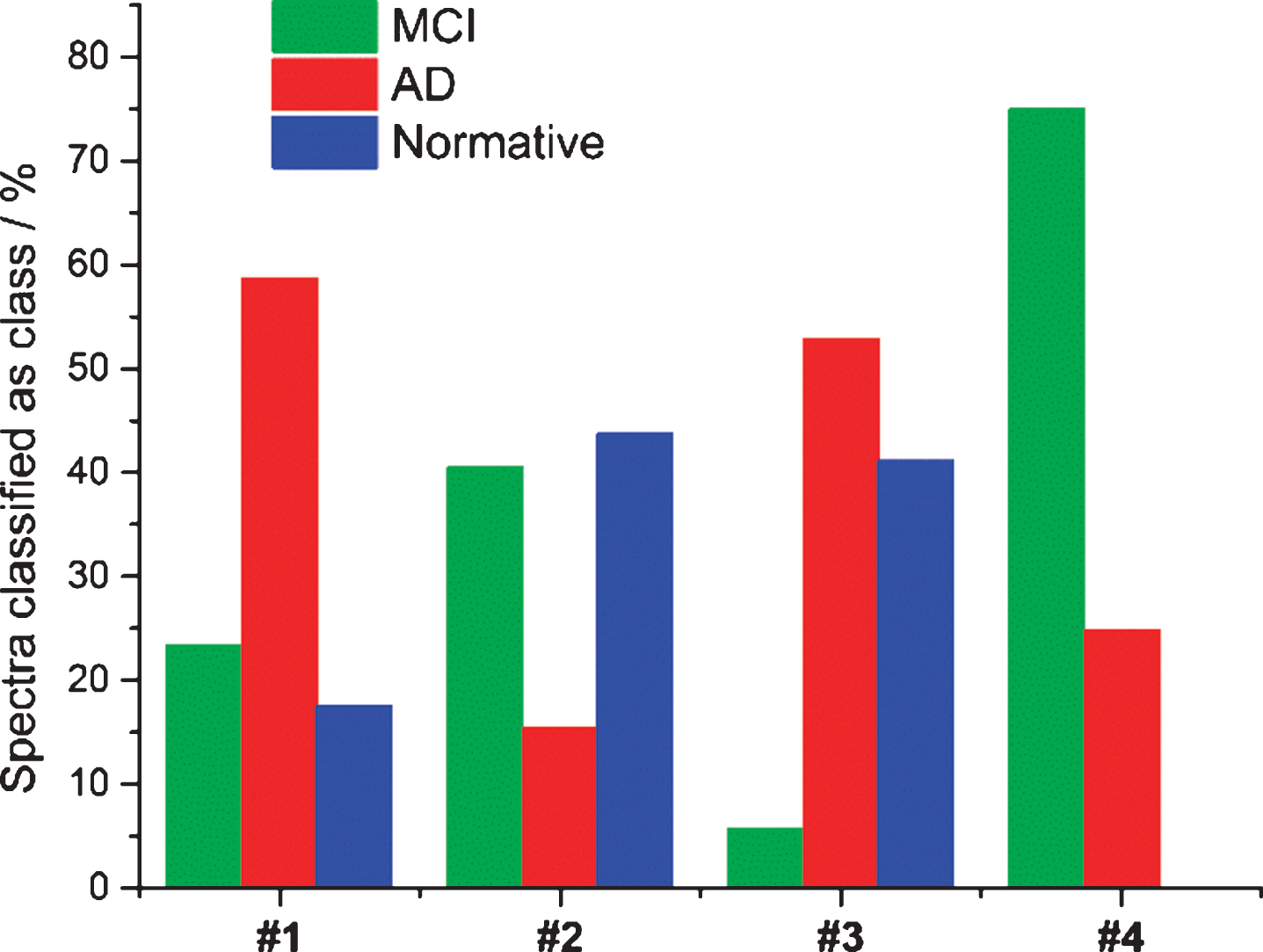
Histogram plotting the results from “blind” external validation of the ANN model. The percent of spectra assigned to three classes: AD (red), MCI (green), and normative (blue) is plotted as the bar heights for all donors.

Lastly, peak intensity ratios were compared between normative and AD samples. Specifically, the ratio between 1320 cm^–1 (internal standard) and 878 cm^–1 (peak which greatly differed between classes and was also selected by GA) were compared. The difference in peak ratios between averaged spectra from normative and AD donors was significant enough for discrimination (see Supplementary Material 4).

DISCUSSION

Many of the bands identified by GA can be assigned to major components of saliva. A summary of those peaks and their assignments as well as tentative contributions can be found in Table 3. Proteins, lipids, and other small biological molecules are mostly responsible for contributing to the average Raman spectra seen in Fig. 1A.

Table 3

Tentative assignments of the most important regions of the Raman spectrum of saliva for discriminating between AD, MCI, and normative classes, as identified by Genetic Algorithm [38 –49]

Peak position (cm^–1)	Band assignment	Tentative contribution
607		Glycerol, Cholesterol
625	(C-C)^a	Proteins (Phe), Lysozyme
643	(C-C)^a	Proteins (Tyr), Lysozyme
702		Cholesterol, Cholesterol ester
719	N⁺(CH₃)₃^b	Phospholipids, Phosphatidylcholine, Sphingomyelin
757	Ring breathing mode	Proteins (Trp)
775	Ring breathing mode	Phosphatidylinositol
830	Ring breathing mode	Proteins (Tyr)
853	Ring breathing mode, (C-C)^b	Proteins (Tyr and Pro)
880	Ring breathing mode, N⁺(CH₃)₃^b	Proteins (Trp), Phosphatidylcholine
903	Acyl chains	Sphingophospholipids
923	(C-C) ring^b	Proteins (Pro), Glucose, Lactic acid
963	Ring vibration	Hypoxanthine
985	Ring breathing mode	Proline
1048	(C-CH₃)^b	Lactic Acid
1068	Acyl Chains	Phospholipids
1126	CH₃^c, (C–O)^b	Proteins (Trp), Lactic Acid
1176	(C-H)^d	Proteins (Tyr and Phe)
1207		Proteins (Tyr and Hydroxyproline)
1272	Ring deformation mode	Proteins (Tyr)
1413	(C = N)^b	Hypoxanthine
1554	(C = C)^b	Proteins (Trp), Lysozyme
1605	(C = C)^d	Proteins (Phe and Tyr)
1667	Amide I	Proteins

^aTwisting, ^bstretching, ^crocking, ^dbending.

Notably, the results of GA are consistent with recent lipidomic and metabolomic studies conducted to determine potential biomarker panels for diagnosing AD. Of interest, metabolic differences in saliva between subjects with AD and healthy controls identified sphinganine-1-phosphate, phenyllactic acid, inosine, and hypoxanthine as influencing diagnostic power [32]. Concurrently, Mapstone et al. identified phospholipids, including phosphatidylcholine, and various amino acids, including proline and phenylalanine, which also contributed toward diagnostic functions [33]. Lysozyme has also been identified as having diagnostic capabilities as its concentration will increase in response to inflammation, a symptom associated with AD [34]. The GA-selected spectral regions are representative of previously determined biomarkers for diagnosing AD and were thus specifically used for further statistical analysis.

The usefulness of saliva for diagnosing diseases has been previously demonstrated. Diagnostic biomarkers within saliva have been used to diagnose various cancers, and bacterial, viral, cardiovascular, and autoimmune diseases [18]. A thorough review of the usefulness of saliva in metabolomics and disease diagnostics can be found elsewhere [18]. Importantly, saliva is completely noninvasive to collect, making it an attractive option over invasive blood or private urine collection. Because of its apparent usefulness and advantages, the analysis of saliva by Raman hyperspectroscopy was considered here for the first time for diagnosing AD.

Raman hyperspectroscopy is uniquely suitable for characterizing micro-heterogeneous environments [35]. Multiple spectra are collected from individual points of a sample, which represent approximately a few hundred femtoliters of volume [36]. The collected spectral data contributes to a three-dimensional hyperspectral data cube (x, y, λ), where x and y are spatial dimensions and λ is the spectral dimension. When machine learning is applied to the data cube, the spatial distribution of biochemical components can be elucidated [37]. This produces a statistically significant characterization of the sample’s heterogeneity and multicomponent composition which can further be used to identify biomarkers, including those present at low average concentrations. Since the entirety of the biochemical composition of a sample is probed, the spectroscopic signature produced for different disease states will be based on the simultaneous integration of multiple biomarkers of the disease, which significantly improves the sensitivity and selectivity of the technique for diagnostic purposes [35].

Furthermore, due to the heterogeneous nature of the sample, the distribution of biochemical components within saliva will be varied. Thus, not every spectrum collected from a single sample will be identical, as some spectra will represent higher or lower local concentrations of biomarkers and biochemical components. This creates the possibility for individual spectra to be misclassified. Because of this, it is important to make donor-level classifications based on spectral-level predictions. Thus, each of the four unknown samples examined during external validation were classified as belonging to the class that the majority of its spectra were assigned. The spectral-level predictions for the four unknown samples are summarized in a histogram (Fig. 2), with the number of spectra assigned to each class scaled to accommodate relative frequencies per donor. The donor-level predictions for each unknown sample are summarized in Table 2 (right-hand side).

External “blind” classification reached 100% accuracy for predicting the class of four unknown donors, showing excellent prediction results and indicating that the model is not majorly overfit. While “blind” external validation was able to show the reliability of the method for diagnosing AD based on saliva, it should be noted this study was designed as a proof-of-concept and the test data set was created using only a few samples. Therefore, more testing is necessary to obtain a strong understanding of the classification accuracy and generalizability of the method. Mean spectra of all four unknown samples are provided in the Supplementary Material 5.

This proof-of-concept study demonstrates the incredible potential of Raman hyperspectroscopy to identify and screen for AD based on analysis of saliva. This technique is sensitive and specific for distinguishing between samples from different classes and is an exemplar non-invasive technique, as saliva can be collected easily through passive drooling. Raman hyperspectroscopy in combination with machine learning was used to successfully differentiate saliva collected from patients with AD or with MCI from normative individuals with an average accuracy of 99%. GA identified areas of spectral data with the strongest differentiation capabilities; the assignments of these identified spectral bands can be attributed to various proteins, amino acids, and lipids, many of which have previously been reported in the literature as potential biomarkers for AD. These important differences in spectral data were utilized by ANN to successfully execute classification between the three different sets of samples. The results were verified through “blind” external validation using an independent dataset to comprehend how well the novel method could classify new unknown data. All four samples used for this task were correctly predicted. Based on such successful results, Raman hyperspectroscopic analysis of saliva is shown here to have a remarkable potential for use as a non-invasive, efficient, and accurate technique for diagnosing AD.

Footnotes

ACKNOWLEDGMENTS

N.M.R was supported by NIH grant T32 GM13206.

Authors’ disclosures available online ().

The supplementary material is available in the electronic version of this article: .

References

What Is Alzheimer’s? Alzheimer’s Association, https://www.alz.org/alzheimers-dementia/what-is-alzheimers, Accessed 5 December, 2018.

Alzheimer’s Association (2018) 2018 Alzheimer’s disease facts and figures. Alzheimers Dement 14, 367–429.

Hardy

, Higgins

(1992) Alzheimer’s disease: The amyloid cascade hypothesis. Science 256, 184–185.

Maccioni

, Muñoz

, Barbeito

(2001) The molecular bases of Alzheimer’s disease and other neurodegenerative disorders. Arch Med Res 32, 367–381.

Jack

, Lowe

, Weigand

, Wiste

, Senjem

, Knopman

, Shiung

, Gunter

, Boeve

, Kemp

, Weiner

, Petersen

(2009) Serial PIB and MRI in normal, mild cognitive impairment and Alzheimer’s disease: Implications for sequence of pathological events in Alzheimer’s disease. Brain 132, 1355–1365.

Sperling

, Aisen

, Beckett

, Bennett

, Craft

, Fagan

, Iwatsubo

, Jack

, Kaye

, Montine

, Park

, Reiman

, Rowe

, Siemers

, Stern

, Yaffe

, Carrillo

, Thies

, Morrison-Bogorad

, Wagster

, Phelps

(2011) Toward defining the preclinical stages of Alzheimer’s disease: Recommendations from the National Institute on Aging-Alzheimer’s Association workgroups on diagnostic guidelines for Alzheimer’s disease. Alzheimers Dement 7, 280–292.

Blennow

, Hampel

, Weiner

, Zetterberg

(2010) Cerebrospinal fluid and plasma biomarkers in Alzheimer disease. Nat Rev Neurol 6, 131–144.

Olsson

, Lautner

, Andreasson

, Öhrfelt

, Portelius

, Bjerke

, Hölttä

, Rosén

, Olsson

, Strobel

, Wu

, Dakin

, Petzold

, Blennow

, Zetterberg

(2016) CSF and blood biomarkers for the diagnosis of Alzheimer’s disease: A systematic review and meta-analysis. Lancet Neurol 15, 673–684.

Ryzhikova

, Kazakov

, Halamkova

, Celmins

, Malone

, Molho

, Zimmerman

, Lednev

(2015) Raman spectroscopy of blood serum for Alzheimer’s disease diagnostics: Specificity relative to other types of dementia. J Biophotonics 8, 584–596.

10.

Liang

, Liu

, Li

, Zhang

A-H

(2016) High-throughput metabolomics analysis discovers salivary biomarkers for predicting mild cognitive impairment and Alzheimer’s disease. RSC Adv 6, 75499–75504.

11.

Yilmaz

, Geddes

, Han

, Bahado-Singh

, Wilson

, Imam

, Maddens

, Graham

(2017) Diagnostic biomarkers of Alzheimer’s disease as identified in saliva using ¹H NMR-based metabolomics. J Alzheimers Dis 58, 355–359.

12.

Charchat Fichman

, Martins Oliveira

, Santos Fernandes

(2011) Neuropsychological and neurobiological markers of the preclinical stage of Alzheimer’s disease. Psychol Neurosci 4, 245–253.

13.

Ryzhikova

, Ralbovsky

, Halamkova

, Celmins

, Malone

, Molho

, Quinn

, Zimmerman

, Lednev

(2019) Multivariate statistical analysis of surface enhanced raman spectra of human serum for Alzheimer’s disease diagnosis. Appl Sci 9, 3256.

14.

Chiappin

, Antonelli

, Gatti

, De Palo

(2007) Saliva specimen: A new laboratory tool for diagnostic and basic investigation. Clin Chim Acta 383, 30–40.

15.

Ross

(1978) Essentials of Human Physiology, Year Book Medical Publishers, Inc., Chicago.

16.

Farquharson

, Shende

, Inscore

, Maksymiuk

, Gift

(2005) Analysis of 5-fluorouracil in saliva using surface-enhanced Raman spectroscopy. J Raman Spectrosc 36, 208–212.

17.

El-Bakary

AAE-S

(2013) Oral fluids and teeth in toxicology. In Evidence-Based Forensic Dentistry, Springer, pp. 189–199.

18.

Zhang

, Sun

, Wang

(2012) Saliva metabolomics opens door to biomarker discovery, disease diagnosis, and treatment. Appl Biochem Biotechnol 168, 1718–1727.

19.

Hanlon

, Manoharan

, Koo

T-W

, Shafer

, Motz

, Fitzmaurice

, Kramer

, Itzkan

, Dasari

, Feld

(2000) Prospects for in vivo Raman spectroscopy. Phys Med Biol 45, R1–R59.

20.

Kong

, Kendall

, Stone

, Notingher

(2015) Raman spectroscopy for medical diagnostics — From in-vitro biofluid assays to in-vivo cancer detection. Adv Drug Del Rev 89, 121–134.

21.

Austin

, Osseiran

, Evans

(2016) Raman technologies in cancer diagnostics. Analyst 141, 476–503.

22.

Sahu

, Dalal

, Naglot

, Aggarwal

, Krishna

(2013) Serum based diagnosis of asthma using Raman spectroscopy: An early phase pilot study. PLoS One 8, e78921.

23.

Bai

, Chen

, Mishra

, Beuerman

, Liu

(2017) Feasibility of quantitatively diagnosing cornea infection using Raman spectroscopy (conference presentation). In SPIE BiOS International Society for Optics and Photonics, San Francisco, California, USA, p. 1005407.

24.

Oshima

, Ishimaru

, Kiyomatsu

, Hino

, Miura

(2018) Evaluation of degenerative changes in articular cartilage of osteoarthritis by Raman spectroscopy. In SPIE BiOS International Society for Optics and Photonics, San Francisco, California, USA, p. 104971A.

25.

Paraskevaidi

, Morais

, Halliwell

, Mann

, Allsop

, Martin-Hirsch

, Martin

(2018) Raman spectroscopy to diagnose Alzheimer’s disease and dementia with Lewy bodies in blood. ACS Chem Neurosci 9, 2786–2794.

26.

Ravina

, Eberly

, Oakes

, Lang

, Dodelet

, Roos

, Harman

, Shoulson

, Schipper

(2015) Plasma near-infrared spectroscopy for diagnosis of idiopathic Parkinson’s disease: The SPIN-PD study. Biomark Med 9, 89–97.

27.

Carmona

, Molina

, Calero

, Bermejo-Pareja

, Martínez-Martín

, Toledano

(2013) Discrimination analysis of blood plasma associated with Alzheimer’s disease using vibrational spectroscopy. J Alzheimers Dis 34, 911–920.

28.

Lednev

(2018) Spectroscopic method for Alzheimer’s disease diagnosis. U.S. Patent No: US 9,891,108.

29.

Fritsch S, Guenther F, Suling M, neuralnet: Training of Neural Networks, R package version 1.32, https://cran.r-project.org/web/packages/neuralnet/index.html, Accessed 17 September 2017.

30.

Günther

, Fritsch

(2010) neuralnet: Training of neural networks. R J 2, 30–38.

31.

Bishop

(1995) Neural networks for pattern recognition, Oxford University Press.

32.

Liang

, Liu

, Zhang

, Jiang

, Xing

, Zhang

A-H

(2015) Metabolomics-based screening of salivary biomarkers for early diagnosis of Alzheimer’s disease. RSC Adv 5, 96074–96079.

33.

Mapstone

, Cheema

, Fiandaca

, Zhong

, Mhyre

, MacArthur

, Hall

, Fisher

, Peterson

, Haley

, Nazar

, Rich

, Berlau

, Peltz

, Tan

, Kawas

, Federoff

(2014) Plasma phospholipids identify antecedent memory impairment in older adults. Nat Med 20, 415–418.

34.

Gruden

, Davudova

, Mališauskas

, Zamotin

, Sewell

RDE

, Voskresenskaya

, Kostanyan

, Sherstnev

, Morozova-Roche

(2004) Autoimmune responses to amyloid structures of Aβ(25–35) peptide and human lysozyme in the serum of patients with progressive Alzheimer’s disease. Dement Geriatr Cogn 18, 165–171.

35.

Ralbovsky

, Lednev

(2018) Raman hyperspectroscopy shows promise for diagnosis of Alzheimer’s. Biophotonics 4, 33–37.

36.

Muro

, Lednev

(2017) Identification of individual red blood cells by Raman microspectroscopy for forensic purposes: In search of a limit of detection. Anal Bioanal Chem 409, 287–293.

37.

Sikirzhytski

, Sikirzhytskaya

, Lednev

(2011) Multidimensional Raman spectroscopic signatures as a tool for forensic identification of body fluid traces: A review. Appl Spectrosc 65, 1223–1232.

38.

Talari

ACS

, Movasaghi

, Rehman

(2015) Raman spectroscopy of biological tissues. Appl Spectrosc Rev 50, 46–111.

39.

Krafft

, Neudert

, Simat

, Salzer

(2005) Near infrared Raman spectra of human brain lipids. Spectrochim Acta A 61, 1529–1535.

40.

Muro

, de Souza Fernandes

, Lednev

(2016) Sex determination based on Raman Spectroscopy of saliva traces for forensic purposes. Anal Chem 88, 12489–12493.

41.

Chen

, Lord

, Mendelsohn

(1974) Laser-excited Raman spectroscopy of biomolecules. V. Conformational changes associated with the chemical denaturation of lysozyme. J Am Chem Soc 96, 3038–3042.

42.

Stone

, Kendall

, Smith

, Crow

, Barr

(2004) Raman spectroscopy for identification of epithelial cancers. Faraday Discuss 126, 141–157.

43.

Daudon

, Protat

, Reveillaud

, Jaeschke-Boyer

(1983) Infrared spectrometry and Raman microprobe in the analysis of urinary calculi. Kidney Int 23, 842–850.

44.

Culka

, Jehlička

, Edwards

HGM

(2010) Acquisition of Raman spectra of amino acids using portable instruments: Outdoor measurements and comparison. Spectrochim Acta A 77, 978–983.

45.

Virkler

, Lednev

(2010) Forensic body fluid identification: The Raman spectroscopic signature of saliva. Analyst 135, 512–517.

46.

Pecul

, Rizzo

, Leszczynski

(2002) Vibrational Raman and Raman optical activity spectra of d-Lactic Acid, d-Lactate, and d-Glyceraldehyde: Ab initio calculations. J Phys Chem A 106, 11008–11016.

47.

Chan

, Taylor

, Zwerdling

, Lane

, Ihara

, Huser

(2006) Micro-Raman spectroscopy detects individual neoplastic and normal hematopoietic cells. Biophys J 90, 648–656.

48.

Ludwig

, Asher

(1988) Ultraviolet resonance Raman excitation profiles of tyrosine: Dependence of Raman cross sections on excited-state intermediates. J Am Chem Soc 110, 1005–1011.

49.

Huang

, McWilliams

, Lui

, McLean

, Lam

, Zeng

(2003) Near-infrared Raman spectroscopy for optical diagnosis of lung cancer. Int J Cancer 107, 1047–1052.