Real-time optimization of active loops for the magnetic field minimization

Abstract

This paper deals with the design and the final implementation of a low-cost active shielding system for the mitigation of magnetic fields generated by electrical installations like power lines or substations. In this paper a new working prototype is built and tested. It is shown that the developed control strategy is effective also for field sources with complex geometries. Moreover, a real-time optimizer is added to the control strategy in order to guarantee the minimization of the source field at any working conditions of the source (i.e. different from the rated power). The control algorithm and the real-time optimizer are fully described in the paper, moreover, their behavior is verified through simulations and experimental tests.

Keywords

Magnetic fields mitigation active shields real-time control

1. Introduction

The magnetic field ( $B$ -field) generated by power-frequency electrical installations has provoked concern in recent decades. Although there is no scientific evidence that prolonged exposure to electromagnetic fields produces long-term effects[1], health effects related to short-term exposure have been established form the basis of both ICNIRP and IEEE exposure limit guidelines [1, 2]. The current literature has well explored the possible mitigation solutions for power lines identifying several options that are suitable for overhead [3, 4] and underground installations [5, 6]. The literature covers also mitigation solutions for more complex field sources and, in this case, the shield is often made by metallic plates [7, 8, 9, 10, 11, 12]. Among the currently available mitigation systems, one solution for having a strong mitigation of the $B$ -field is the use of active shielding systems [13]. This technique consists in a coil (or a set of coils) where an alternating current (with a certain magnitude and phase) is injected by an external equipment in order to generate a $B$ -field which counteracts the original one, resulting in a mitigated $B$ -field. This technique has shown to be attractive not only for the reduction of the $B$ -field in wide areas close to overhead lines [14, 15, 16, 17], but also in MV/LV substations [18, 19] and other industrial applications [20]. However, the need of an external power supply increases the complexity of the shielding system in comparison with other mitigation techniques, so its properties must be selected carefully during the design process of the active shield. In addition, the mitigation system must have a controller to guarantee the optimal compensation at any time due to variations on the loading conditions of the field source. In this sense, previous works employed control techniques based on the implementation of a proper transfer function in an electronic system [20], which is generally an analogical system. Nonetheless, the introduction of a microcontroller could extend the possibilities of control, which would be not limited to a transfer function anymore. In this regard, this paper deals with the design and application of a low-cost microcontroller-based system for the active shielding of the $B$ -field generated by power lines and MV/LV substations. In reference [21] a first prototype has been developed. In this paper the controller is improved by adding new hardware and software features in order to provide better mitigation results. In particular, the new prototype is more flexible and adaptable to different $B$ -field sources and its loading conditions thanks to the implementation of a “perturb and observe” control algorithm. In the following sections, the software of the new prototype is fully described, and several numerical results are also presented.

2. Prototype description

A first prototype for the active shield was already developed and successfully applied to the mitigation of the $B$ -field generated by a three-phase line [21]. The whole system is designed by a two-stage procedure. The first stage assumes standard working conditions (e.g. three-phase balanced system) providing the geometry of the active loops that makes possible to minimize the magnetic fields in the desired region of interest. The optimization is performed by genetic algorithms and all details can be found in [22]. The second stage is the design of the control algorithm which guarantees the minimization of the magnetic field also for non standard working conditions (e.g. three-phase unbalanced system). This paper focuses on a significant improvement of the second stage. An new version of the control algorithm has been developed with the following new features: i) possibility to drive $n$ shielding loops, ii) possibility to measure and analyze the $B$ -field at $m$ points, iii) possibility to run a real-time optimization tool called “minimum field tracker” (details will be given later). The hardware is shown in Fig. 1.

Figure 1.

Prototype of the active shield controller.

A detailed description of the minimum field tracker (MFT) algorithm will be given in the rest of the paper, here we briefly recall the basic working principle of the active koops developed in [21]. The simplest layout of the active shield is based on the following expressions:

$\displaystyle\bar{B}_{j}=\bar{B}_{j,s}+\bar{B}_{j,sh}=\bar{\alpha}_{j}\bar{I}_% {s}+\bar{\beta}_{j}\bar{I}_{sh}$ (1) $\displaystyle\bar{I}^{\prime}_{sh}=\bar{\gamma}\bar{I}_{s}$ (2)

All of the above quantities are complex numbers, more precisely, they are phasors when related to magnetic fields or currents. Subscript $j$ is used to identify the $j$ th component of the field. $\bar{B}_{j}$ is the total field at a given point, $\bar{B}_{j,s}$ is the magnetic flux density created by the source and $\bar{B}_{j,sh}$ is the compensation field created by the shield. $\bar{I}_{s}$ is a current selected to represent the source field. For a three-phase system one can select arbitrarily the current of phase 1, 2 or 3. $\bar{\alpha}_{j}$ is the ratio between $\bar{B}_{j,s}$ and $\bar{I}_{s}$ , it depends only on the geometry of the source under standard working conditions. $\bar{I}_{sh}$ is the shielding current flowing in the active loop and $\bar{\beta}_{j}$ is the coefficient that links the shield current to the compensation field $\bar{B}_{j,sh}$ . For a system with only one loop $\bar{\beta}_{j}$ is a scalar quantity, however, in systems with more than one loop a single current $\bar{I}_{sh}$ can represent the behavior of a group of loops. For this reason, also $\bar{\beta}_{j}$ is presented here as a complex number. $\bar{\alpha}_{j}$ and $\bar{\beta}_{j}$ are both computed at the end of the first stage of the design when the geometry of the active loop is known (more details in [22]). Equation (1) is a general expression that gives the total field for all possible working conditions of the source (described by $\bar{I}_{s}$ ) and the shield (described by $\bar{I}_{sh}$ ). For a given value of $\bar{I}_{s}$ , the shielding current that makes it possible to minimize the total field is provided by Eq. (2). The optimal shielding current is identified by the variable $\bar{I}^{\prime}_{sh}$ and the link between the source current and the optimal shielding current is called $\bar{\gamma}_{j}$ . Once again, $\bar{\gamma}_{j}$ is obtained at the end of the first stage of the design described in [22].

Figure 2.

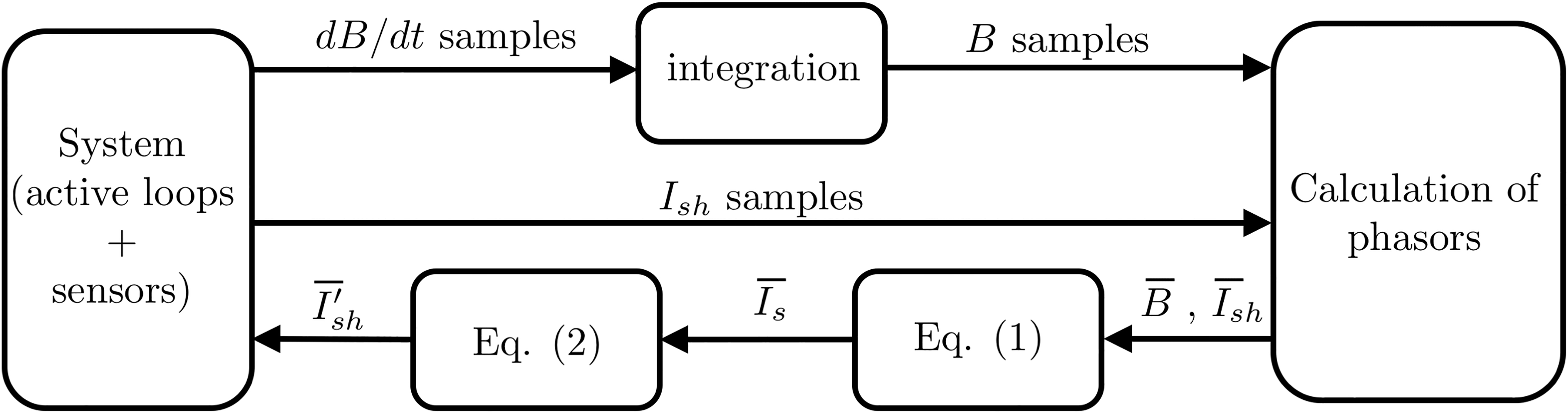
Scheme of the control algorithm.

The first prototype was based only on the above mentioned two equations. Its working principle is explained in Fig. 2. Basically, at a given instant of time, the shielding current and the time derivative of the total magnetic flux density are measured in time domain. The magnetic flux density is then obtained by time integration and provided to the microcontroller that calculates the phasors associated to the total magnetic flux density and the shielding current. Equation (1) is then used in cascade to estimate the source current and to adjust, according to Eq. (2), the shielding current.

2.1 Experimental validation

The performance of the prototype was analyzed on a simple case study tested under controlled conditions. A 6 meter long power line were assembled in a laboratory and an active shield made of only one loop were designed [21]. Some measurements were carried out along the inspection line to check the validity of the optimal solution and the performance of the control system. The main results are reported in Table 1, where data are related to a source current equal to $I_{s}=$ 25 A. As it can be observed, the results are in good agreement with the analytical calculations derived from the optimization procedure, hence validating the rationale on which the whole system is based: design, modeling and control system. The small differences observed are mainly caused by possible deviations in the 3D model in comparison to the actual installation. For this reason, a “perturb and observe” algorithm has been developed to improve the effectiveness of the shielding system.

Table 1
B-field expressed in $\mathrm{\mu T}$ with and without shielding system

x (m)	Simulation source	Measure source	Simulation total	Measure total
	field	field	field	field
0	1.910	2.078	0.346	0.430
0.5	1.743	1.867	0.338	0.356
1	1.358	1.385	0.263	0.279
1.5	0.959	0.957	0.179	0.168
2	0.654	0.648	0.117	0.120
2.5	0.447	0.443	0.078	0.072
3	0.311	0.340	0.053	0.070

Figure 3.

Experimental setup: power line made of three conductors 6 meter long with spacing of 0.5 m. The active shield is made of one loop 0.1 m above the power line, it is 6 m long, it is wide 1.34 m. The geometry of the loop comes from the optimal design as well as the optimal current [21, 22].

3. Perturb and observe algorithm

As mentioned earlier, a “perturb and observe” algorithm has been implemented in the prototype under analysis. This technique has been preferred among other possibilities because it is characterized by a very low price-performance ratio [23]. Its goal is the searching of the actual optimal shielding current under conditions that are different from the design ones. In fact, the setpoint calculated offline by the optimization process might not be perfect due to: i) simplifying assumption on the 3D model that, consequently, it is not exactly compliant with the actual geometry and/or the properties of the materials. ii) Loading condition of the power line that differs from the rated one. For instance: unbalanced load or partial load working conditions.

In addition, the measure of $B$ -field and $\bar{I}_{sh}$ might be affected by errors that lead to a setpoint different from the optimal one. To overcome these issues, the new algorithm perturbs the parameter $\bar{\gamma}$ during the runtime and it evaluates the effect on the total $B$ -field in order to search the best setpoint. This new algorithm has been named “minimum field tracker”. Its approach is similar to the maximum power point tracker (also known as MPPT) used in the inverters for photovoltaic applications [23] but, instead of working on a scalar quantity (which is the duty cycle of the buck converter for the MPPT), it works on a complex number ( $\bar{\gamma}$ ). The variables that are perturbed during the runtime are: i) the magnitude of $\bar{\gamma}$ for each shielding loop, ii) the angle of $\bar{\gamma}$ for each shielding loop. For example, an active shield with one loop has 2 optimization variables, the magnitude and the angle of the single available $\bar{\gamma}$ values. The MFT algorithm starts perturbing a first variable (for instance the magnitude of $\bar{\gamma}$ ) and it observes the variation of the $B$ -field. Actually, the MFT observes the ratio $B$ -field/ $I_{s}$ called performance indicator to take into account possible variations of the load profile during the observation time. In fact, the normalization of the $B$ -field with the module of the current $\bar{I}_{s}$ makes it possible to compare the magnetic flux density at different loading conditions. The MFT proceeds checking if the performance indicator increases or not. If it is increased, the MFT changes sign to the perturbation and it observes the $B$ -field again, otherwise it continues to perturb the variable with the same sign. These operations are repeated until a stable condition is reached and, after a given delay, the loop starts again perturbing another variable (for instance the angle of $\bar{\gamma}$ ). A more schematic explanation of the MFT working principle is given by the pseudocode in Fig. 4.

Figure 4.

Pseudocode of the MFT working principle. In this paper the value of $N$ is equal to 5 (line 9 of the code) and the delay is equal to 0.2 s (line 21 of the code).

The inspection point used as feedback for the MFT can coincide with the one used for Eq. (1) but this is not always possible and neither mandatory. If the complexity of the source increases, usually more than one feedback point can be used. Although the definition of the number and the position of such inspection points is hard to be generalized, one chief criterion can be considered. The measurement at the inspection point is used to assess the source current $\bar{I}_{s}$ by means of Eq. (1). Therefore, it is mandatory to not collocate the inspection points too close to the shield otherwise $\bar{B}_{j}\approx\bar{B}_{j,sh}$ . If that happens, the assessment of the source current becomes very inaccurate or even not possible.

3.1 Experimental test

The MFT algorithm has been tested experimentally on the laboratory setup described in Fig. 3. The MFT is stressed setting intentionally a wrong value for the $\bar{\gamma}$ parameter: the optimal design suggests the use of this value $\bar{\gamma}_{\textit{opt}}=$ 0.631 $\exp(j2.56)$ whereas the initial value is deliberately set to $\bar{\gamma}_{0}=0.35\exp(j1.8)$ .

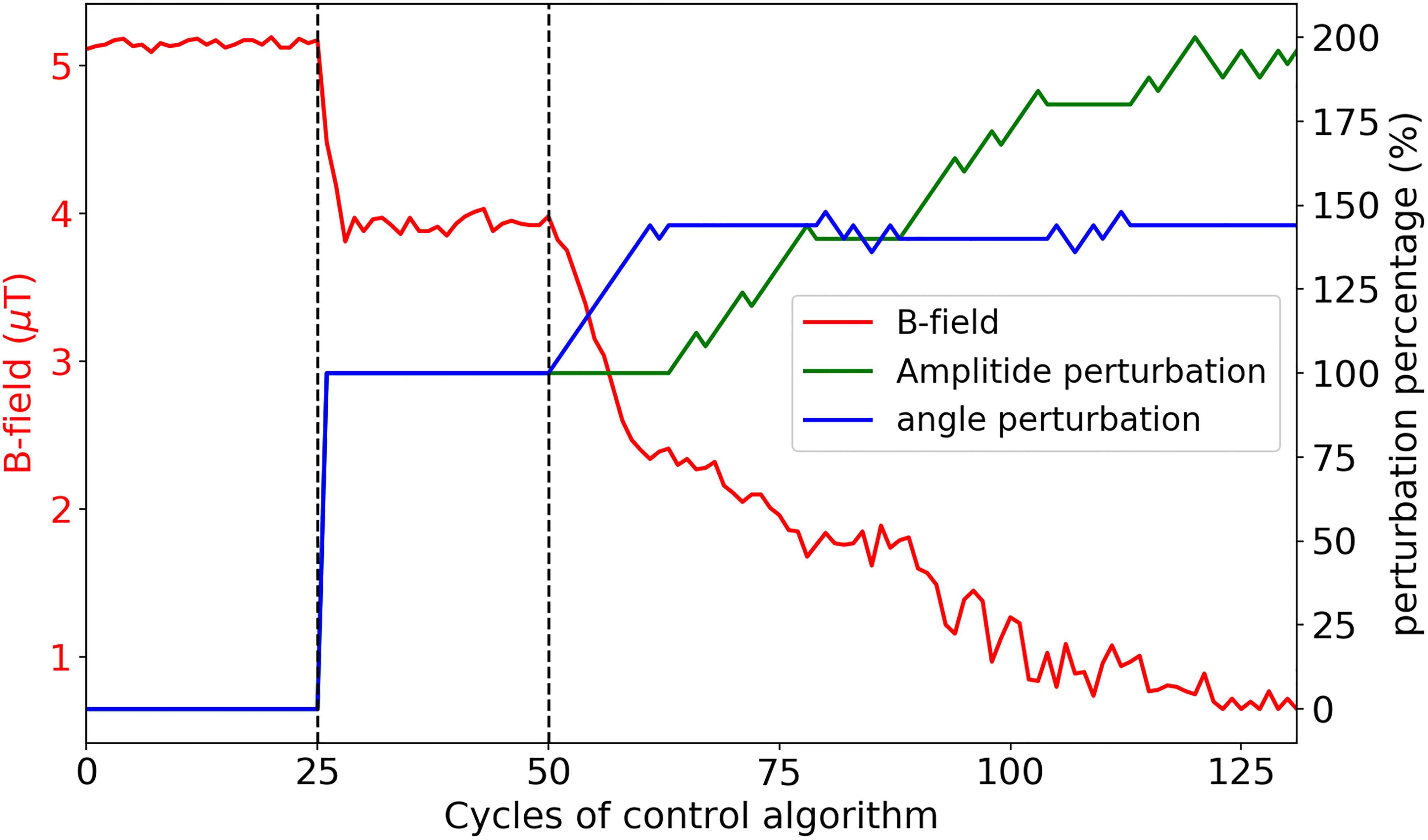
The test carried out is summarized by Fig. 5. The x coordinate represents the cycles of the control algorithm (to evaluate the absolute time one has to multiply by the conversion factor 0.2 ms/cycle). In the first part of the experiment the shielding system is off and the magnetic flux density (red curve to be read on the left y-axis of 5) is approximately 5 ${\mu T}$ . At the 25th cycle the active shield is turned on (but the MFT is off) and the $B$ -field decreases immediately to 4 ${\mu T}$ . Since we intentionally set a non-optimal value of $\bar{\gamma}$ this is not the best performance of the shield. At the 50th cycle the MFT is turned on and it perturbs first the angle and then the magnitude of $\bar{\gamma}$ until a stable condition is reached. The perturbation has to be read on the right y-axis of Fig. 5. At the end of the process the $B$ -field is lower than 1 ${\mu T}$ . The final value of $\bar{\gamma}$ corresponding to the stable condition is $\bar{\gamma}=0.69\exp(j2.59)$ . It is worth noting that the final value is very close the optimal one: $\bar{\gamma}_{\textit{opt}}=0.631\exp(j2.56)$ .

Figure 5.

Experimental test of the MFT algorithm on a three-phase power line. Up to the 25th cycle the active shield is off. $B$ -field values at the inspection point is represented in red and had to be read on the left y-axis. The other two curves represent the percentage perturbation of the $\gamma$ parameter and they have to be read on the right y-axis. From the 25th cycle to the 50th cycle the active shield is on and the MFT is off. At the 50th cycle the MFT is turned on and the plot range goes until the stable (minimum field) condition is found.

Figure 6.

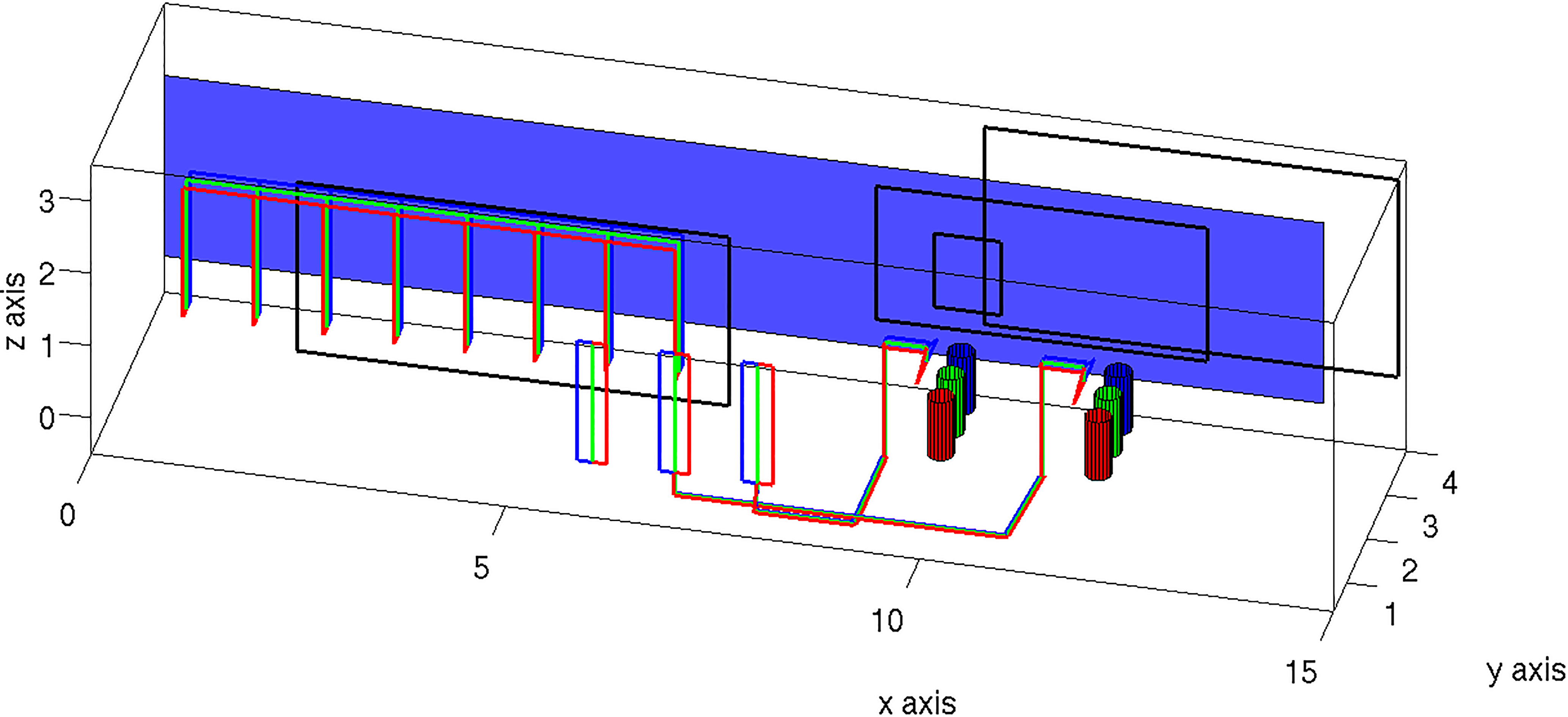
Geometry of the substation (red, blue and green conductors represents the phase 1, 2 and 3, respectively). The active loops are represented in black color and the inspection plane in violet.

4. Effectiveness of the MFT on complex sources

A previous work discussed the possibility to use active loops on complex field sources like substation [22]. Satisfactory results were obtained and, therefore, the active loops can be considered as an alternative shielding solutions also for complex field sources. In reference [22], however, the authors considered a magnetic field source at its rated power with possible homogeneous variation of the loading condition. This is a strong limitation because a complex substation can be divided in more than one section that could be operated independently. A simple example is provided in Fig. 6 where a substation with two 630 kVA MV/LV cast resin transformers is shown. The standard design takes into account all the components at their rated power but several other working conditions can be found. For example, if the two transformers supply two independent loads, an extremely different condition would be: one transformer at the rated power and the other transformer working at no load conditions. Theoretically, for each working behavior there is an optimal shield configuration but, of course, only one has to be designed. In this section we will show that the MFT algorithm makes it possible to overcome the limitations assumed in [22].

Figure 7.

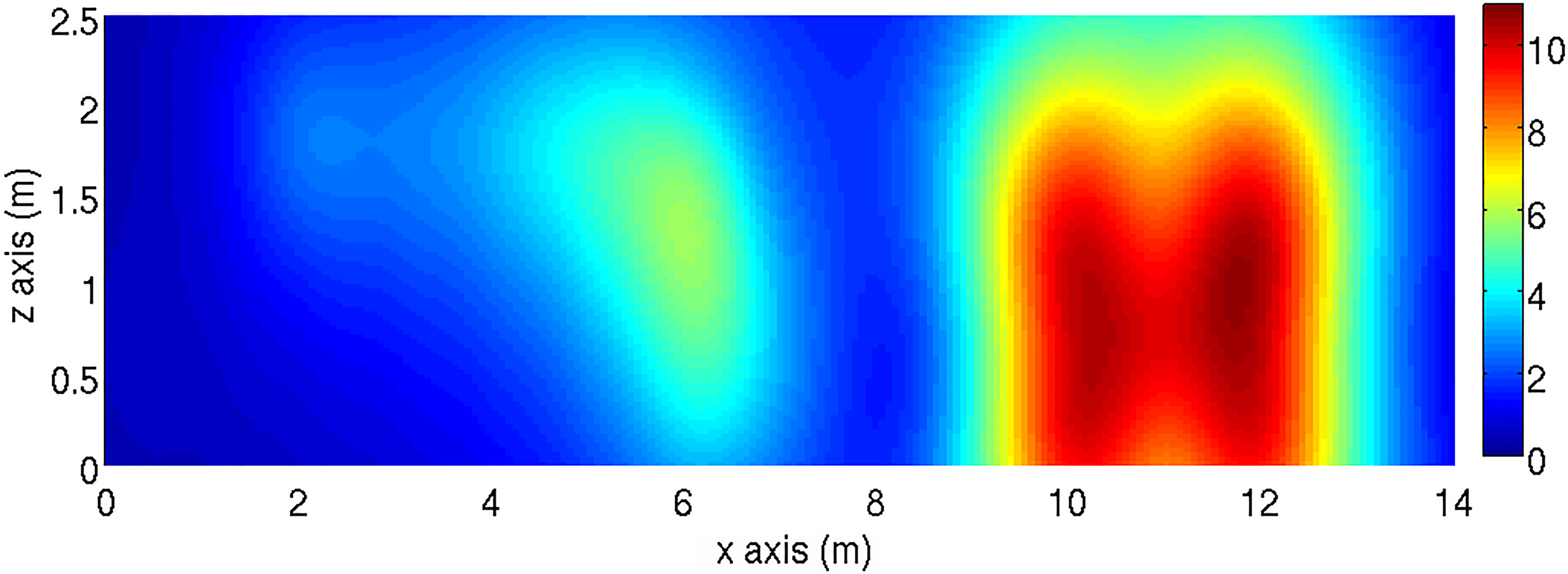
$B$ -field on the inspection plane with all the components at rated power and the shield is off. Value in $\mathrm{\mu T}$ .

Figure 8.

Mitigation of the $B$ -field on the inspection plane with all the components at rated power. The optimal active loops system is turned on. Value in $\mathrm{\mu T}$ .

Figure 6 represents the geometry of an actual substation that includes: two 630 kVA MV/LV cast resin transformers, one MV switchgear with seven cells and one LV switchgear. The active shield is made of 4 loops represented in black color. They are all located on the wall corresponding to $y=4$ m because it was forbidden by the local distributor to use the other walls. The represented geometry comes from an optimization procedure [22] based on the working configuration at rated power. The goal is to minimize the average $B$ -field in a target volume that extends beyond the wall at $y=4$ m. In this paper we present the $B$ -field on the inspection plane that corresponds to the surface of the target volume which is closest to the substation. This surface lays on the wall at $y=4$ m and it is represented in violet color in Fig. 6.

Figure 9.

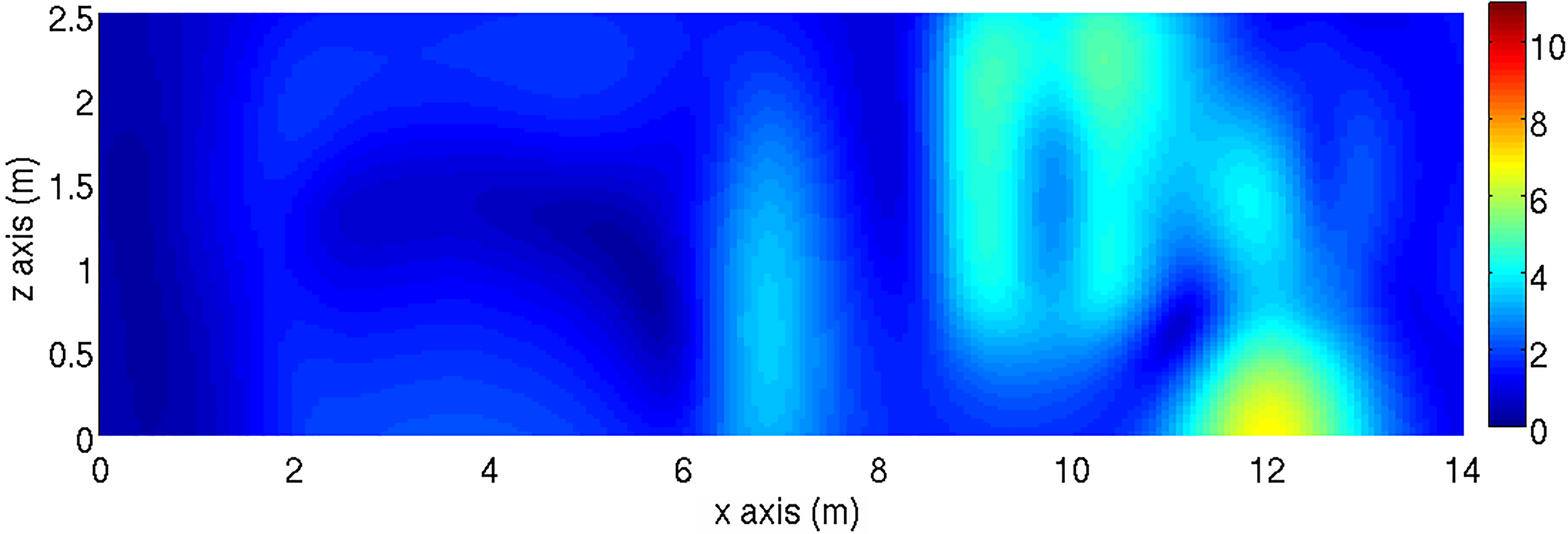
$B$ -field on the inspection plane when only one transformer and its related distribution/cables are active and the shield is off. Value in $\mathrm{\mu T}$ .

Figure 10.

Mitigation of the $B$ -field on the inspection plane when only one transformer and its related distribution/cables are active. Value in $\mathrm{\mu T}$ . This is a fictitious case in which the $B$ -field is mitigated by the optimal active loops system for this configuration.

First the working condition at rated power is analyzed. Figure 7 shows the $B$ -field created by the source at rated power on the inspection plane. Figure 8 shows the reduction obtained by the active loops system optimized for such working condition. It is noticeable the significant reduction obtained.

Now let us analyze a considerable variation of the working condition by turning off one of the transformer (the left one in Fig. 6). The source field on the inspection plane becomes the one represented in Fig. 9. As already mentioned, a new working condition would require a new optimal design. Even if it is impossible to modify the geometry of the active loops system in the reality, we evaluated this new confutation and we tested its performance. The reduction of the $B$ -field is shown in Fig. 10.

Now, coming back to the impossibility of changing the geometry of the active loops system once it is designed, we are going to show what happen if the active loops system optimized under rated conditions is used to mitigate the magnetic flux density created by only one transformer (and its related cables) in the substation. This result is shown in Fig. 11. It is apparent that the shield is not providing any mitigation and, on the contrary, the $B$ -field is increased at some points of the inspection plane.

Figure 11.

Mitigation of the $B$ -field on the inspection plane when only one transformer and its related distribution/cables are active. Value in $\mathrm{\mu T}$ . In this case the active loops system optimized at rated power is used. It is apparent that the mitigation is not satisfactory and the $B$ -field is even increases at some points.

Finally, starting from the condition of Fig. 11 the MFT is activated and, after some cycles, the stable condition of Fig. 12 is obtained. Figure 12 shows a significant reduction factor. This result should be compared with the one obtained using the optimal active loops system for this configuration represented in Fig. 10. Even if the MFT is unable to reach the reduction factor of the optimal configuration, it makes possible a significant reduction that is comparable to the optimal one. Moreover, the MFT guarantees that the $B$ -field will never be increased by the active loops.

Figure 12.

Mitigation of the $B$ -field on the inspection plane when only one transformer and its related distribution/cables are active. Value in $\mu T$ . In this case the active loops system optimized at rated power is used. The map of the $B$ -field represents the sable condition obtained by turning on the MFT. The improvement with reference to Fig. 11 is noticeable.

5. Conclusions

This paper presents the new features of a previously developed prototype of a low-cost active shielding system. The prototype is based on a low-cost control hardware ( $\approx$ 100 €), and now it has been improved by extending the hardware and the firmware features. A perturb and observe algorithm called minimum field tracker has been developed. The MFT makes more flexible and adaptable the shielding system to complex $B$ -field sources, like MV/LV substations, where the loading conditions may vary without homogeneity in all the components. The performance of this new algorithm is analyzed in two situations: three-phase line in flat configuration and MV/LV substation. The results show that the MFT algorithm is able to improve the mitigation results by compensating possible differences between the data employed in the design stage and the actual installation.

On the other hand, since the active shield is designed considering the most common loading conditions of the $B$ -field source or the rated loading conditions, the control algorithm has to react to changes of the working point of the source. In this situation, the new algorithm has proven to be quite efficient, recalculating the right shielding currents to be injected in the active shield which was optimized for very different loading conditions. This leads to a shielding factor which is comparable to the optimum one.

References

ICNIRP, Guidelines for limiting exposure to time-varying electric and magnetic fields (1 Hz to 100 kHz). Health Phys 99(6) (2010), 818–836.

C95.6 – IEEE Standard for Safety Levels with Respect to Human Exposure to Electromagnetic Fields, 0–3 kHz.

Reta-Hernández

and Karady

G.G.

, Attenuation of low frequency magnetic fields using active shielding. Electr. Power Syst. Res. 45 (1998), 57–63.

Ippolito

and Siano

, Using multi-objective optimal power flow for reducing magnetic fields from power lines, Electr. Power Syst. Res. 68 (2004), 93–101.

Habiballah

I.O.

Farag

A.S.

Dawoud

M.M.

and Firoz

, Underground cable magnetic field simulation and management using new design configurations, Electr. Power Syst. Res. 45 (1998), 141–148.

Canova

Bavastro

Freschi

Giaccone

and Repetto

, Magnetic shielding solutions for the junction zone of high voltage underground power lines, Electr. Power Syst. Res. 89 (2012), 109–115.

Barbarics

and Kis

, Magnetic shielding on low-frequency, International Journal of Applied Electromagnetics and Mechanics 13(1–4) (2001), 441–446.

Bottauscio

Chiampi

Chiarabaglio

Fiorillo

Rocchino

and Zucca

, Role of magnetic materials in power frequency shielding: numerical analysis and experiments, In IEE Procedings of Generation, Transmission and Distribution 148 (2001), pp. 104–110.

Bottauscio

Chiampi

and Manzin

, Numerical analysis of magnetic shielding efficiency of multilayered screens, IEEE Trans. Magn. 40(2) (2004), 726–720.

10.

San Segundo

H.B.

and Roig

V.F.

, Reduction of low voltage power cables electromagnetic field emission in MV/LV substations, Electr. Power Syst. Res. 78 (2008), 1080–1088.

11.

Saito

, Open-type magnetic shielding method, International Journal of Applied Electromagnetics and Mechanics 33(3–4) (2010), 891–899.

12.

Bavastro

Canova

Giaccone

and Manca

, Numerical and experimental development of multilayer magnetic shields, Electric Power Systems Research 116 (2014), 374–380.

13.

Mitigation techniques of power frequency magnetic fields originated from electric power systems. Technical Report Working group C4.204, International Council on Large Electric Systems (CIGRE’), 2009, ISBN: 978-2-85873-060-5.

14.

Jonsson

and Sjödin

J.O.

, Optimized reduction of the magnetic field near Swedish 400 kV lines by advanced control of shield wire currents. test and economic evaluation, IEEE Transactions on Power Delivery 9(2) (April 1994), 961–969.

15.

Okazaki

Yanase

and Sugimoto

, Active magnetic shielding with magneto-impedance sensor, International Journal of Applied Electromagnetics and Mechanics 13(1–4) (2001), 437–440.

16.

Cruz

Izquierdo

Burgos

Ferrer

Llanos

and Pacheco

, Magnetic field mitigation in power lines with passive and active loops, In: Proc. CIGRE, 2002, pp. 36–107.

17.

Barsali

Giglioli

and Poli

, Active shielding of overhead line magnetic field: Design and applications, Electric Power Systems Research 110 (May 2014), 55–63.

18.

Buccella

Feliziani

and Prudenzi

, Active shielding design for a MV/LV distribution transformer substation, In 3rd International Symposium on Electromagnetic Compatibility (May 2002), pp. 350–353.

19.

Garzia

and Geri

, Active shielding design in a full 3D space of indoor MV/LV substations using genetic algorithm optimization, In IEEE International Symposium on Electromagnetic Compatibility 1 (August 2003), pp. 197–202.

20.

Sergeant

P.L.

Van den Bossche

and Dupré

, Hardware control of an active magnetic shield, IET Science, Measurement & Technology 1(3) (May 2007), 151–159.

21.

Canova

del Pino López

J.C.

Giaccone

and Manca

, Active shielding system for elf magnetic fields, IEEE Transaction on Magnetics 51(3) (2015).

22.

del Pino López

J.C.

Giaccone

Canova

and Cruz-Romero

, Design of active loops for magnetic field mitigation in MV/LV substation surroundings, Electric Power Systems Research 119 (2015), 337–344.

23.

Femia

Petrone

Spagnuolo

and Vitelli

, Optimization of Perturb and Observe Maximum Power Point Tracking Method, IEEE Transactions on Power Electronics 20(4) (Jul 2005), 963–973.

Real-time optimization of active loops for the magnetic field minimization

Abstract

Keywords

1. Introduction

2. Prototype description

Table 1 B-field expressed in μ ⁢ T with and without shielding system

References

Table 1
B-field expressed in $\mathrm{\mu T}$ with and without shielding system