Reactive-power-based MRAC for rotor resistance and speed estimation in bearingless induction motor drives

Abstract

The reactive power-based model reference adaptive controller (MRAC) is presented in this paper in detail to estimate rotor resistance online. This controller can maintain rotor flux orientation of bearingless induction motor (BIM) driven by indirect vector control. The instantaneous and steady state reactive power of the rotating part of the BIM are selected in the MRAC as reference model and adjustable model, which automatically protects the entire system from any effects of stator resistance. In addition, this proposed formation of MRAC is independent of the requirement for the estimation of any flux in the calculation process. Therefore, this scheme is not influenced by the integration, and the problems like saturation and drift can be ignored. At zero speed, this scheme will estimate the rotor resistance more accurately. A speed sensorless scheme can be proposed after adding flux estimators to the MRAC. The effectiveness of the proposed scheme has been verified in MATLAB/SIMULINK.

Keywords

bearingless induction motor model reference adaptive controller reactive power estimation sensorless

1. Introduction

The AC motor is widely used in high-performance industrial applications, but it is hard to satisfy the needs of modern industry [1–3]. Therefore, a motor supported by the magnetic bearing has emerged. However, it still has some shortcomings, such as more power consumption for magnetic suspensions, limited critical speed, less rotor stiffness, and so on [4–6]. The bearingless motor is a new type of AC motor that places both the suspension force windings and the torque windings in the stator slots of the motor. The two sets of windings interact to create a radial suspension force that stabilizes the rotor [7–10]. Compared with the motor supported by the magnetic bearing, the BIM has higher axial utilization, which provides more power for the motor operation at high speed and super high speed [11–13]. The size of the bearingless motor is smaller and the space utilization is higher. Bearingless motors have obvious reduction in losses during operation and the operating consumption is relatively low [14–16]. Therefore, the BIM has popularized in the field of medical, aerospace and high-speed hard disk [17,18].

The BIM is a system with of strongly coupled nonlinearity characteristics. To achieve decoupling control between the excitation component and the torque component in the stator current, the rotor flux-oriented vector control is adopted by BIM. The rotor flux-oriented vector control takes the orientation of the magnetic field as the reference orientation of the coordinate system, and the magnitude orientation of the current vector is represented by the instantaneous value [19–21]. Then, the AC motor model can be equivalent to the DC motor for control. However, the rotor resistance is required for adjusting the slip-frequency, which makes the scheme rely on the accuracy of the motor parameters [22–24]. In the actual motor parameters, the rotor resistance will vary with the operating temperature, but the rotor resistance in the controller is a constant. If the compensation for variety is ignored, it will lead to the inaccuracy of the field orientation and couple between the excitation component and the torque component in the stator current of torque windings [25–28]. The performance of the entire drive system is influenced by this couple. To eliminate the effects of rotor resistance, many algorithms for online rotor resistance identification have been proposed [29–32].

Signal injection-based method, as a kind of method for identifying the motor parameter, is mentioned in [33] and [34]. This method obtains the motor parameters by injecting characteristic signals into the system. However, this method has certain limitations on the identification of the rotor resistance. To some extent, it destroys the normal operation state of the motor, and sometimes even generates strong torque ripple, so it is rarely used in practical systems. In [35], observer-based method is used for motor parameter identification in nonlinear systems. It mainly contains extended kalman filter (EFK) and extended luenberger observer (ELO). The basic idea is to take the required motor parameters as the internal state of the system. The theoretical identification algorithm of the observer is used to obtain the required parameters. However, the matrix operations and careful preprocessing are required in each step of this method. Due to the large amount of computations and memory requirements, even the reduced-order Kalman filter is used, it is still difficult to be used in actual vector control. MRAS is another method for motor parameter identification. It is one of the adaptive control methods proposed for the uncertainties existing in the system. The proposed model reference adaptive controller (MRAC) based rotor resistance estimation scheme contains two kinds of model, one of which contains the rotor resistance as an adjustable model, and the other as a reference model. Both models have the same physical meaning of output. According to the certain adaptive law, the deviation of the two model outputs is used to dynamically update the rotor resistance of the adjustable model. Then the error between the outputs of the two models will tend to zero. When the steady state is reached, the parameter value in the adjustable model is the actual rotor resistance. The research on parameter identification of MRAS mainly focuses on selection of various models, such as, rotor flux based [36], reactive-power based [37–39], electromagnetic torque based [40]. There are numerous other identification methods for motor parameters identification, such as fuzzy artificial neural networks [41], recursive least squares [42]. Some methods are also based on various algorithms [43–45].

In this paper, the use of reactive power-based model reference adaptive controller in BIM is described detailly to realize rotor resistance identification. The estimation of rotor flux is not required in the proposed MRAC. It is worth noting that MRAC-based schemes have been reviewed [46–48]. However, most of them do not have comprehensive analysis of stability and sensitivity, and the identification of the rotor flux is also required in the calculation. Therefore, at low speeds they suffer from the problems associated with the integrator and the relatively low accuracy achieved in the calculations. The most important contribution of the proposed MRAC in this paper are the utilization of instantaneous reactive power and the steady-state reactive power of the rotating part of the BIM in the reference model and adjustable model. The identification for rotor resistance in the BIM is established based on this scheme. Finally, the simulation is carried out in MATLAB/SIMULINK according to the proposed scheme.

This paper is composed of the following parts. In the second part, the principle of the suspension force generation in BIM is introduced. In the third part, the reactive power-based MRAC controller is constructed and related stability principles are analyzed. In the fourth part, the rotor field-oriented vector control system of the BIM based on MRAC is established. In the fifth part, the relevant simulations are carried out. In the sixth part, the use of MRAC is improved into the speed sensorless scheme and the corresponding results are obtained in the simulation. Finally, some conclusions are summarized in the seventh part.

2. Principle of radial suspension force generation

Two sets of three-phase windings with different pole pairs are stacked in the stator of the bearingless induction motor, one is torque windings whose pole pair number is p ₁ and another is suspension force windings whose pole pair is p ₂. Controllable radial suspension force can be generated when the bearingless induction motor satisfies the following conditions (1) p ₂ = p ₁ ± 1, (2) the currents in two sets of windings have the same electrical angle frequency [49–52].

According to the electromagnetic theory, it is known that there are two kinds of electromagnetic forces in ordinary BIM: Lorentz force and Maxwell force. In the BIM, the principal of radial suspension force generation is Maxwell force, also called magnetic resistance force. Compared with Maxwell force, Lorentz force not only generates electromagnetic torque, but also generates small amount of radial suspension force. The principle of radial suspension force generation is illustrated in Fig. 1. The effective number of the turns of torque windings and suspension force windings are assumed to N ₁ and N ₂, respectively. The currents flowing into torque windings and suspension force windings are i ₁ and i ₂ and generate fluxes 𝜓₁ and 𝜓₂ respectively. Mutually perpendicular rotor position axes are represented by x and y. When the current flowing into windings in the direction shown in Fig. 1, the direction of the upper fluxes 𝜓₁ and 𝜓₂ is the same, the air gap flux density is increased, and the lower fluxes 𝜓₁ and 𝜓₂ are opposite in direction, so the air gap flux density is decreased. The radial force F _y produced by the rotor of the motor along the positive direction of y due to the unbalanced air gap flux density. If the direction of current flowing into the suspension force windings is reversed, radial suspension force can be generated in the opposite direction of y. Similarly, the radial force in the x direction can be obtained by passing a current perpendicular to I ₂ in the suspension force windings N ₂. Therefore, the stable suspension performance of the rotor of the BIM can be achieved by controlling the magnitude and direction of the current in the suspension force windings.

Fig. 1.

Principle of radial suspension force generation.

Fig. 2.

Structure of MRAC.

3. Proposed scheme

3.1. Basic structure of MRAC

In the proposed MRAC (Fig. 2), the instantaneous reactive power (Q _ref) and steady state reactive power (Q _est) of the rotating part of the BIM can be calculated by using the reference model and adjustable model, respectively. The difference between the reference model and adjustable model is that the reference model depends on ω_s and the adjustable model is independent of ω_s. The error signal is derived from the formula ϵ = Q _ref − Q _est. It is fed into the adaptation mechanism block and generals the estimated slip speed (ω_s,est). The whole driving process is shown in Fig. 3. The block diagram includes the rotor resistance update block. It is used to make the IFO-controller more insensitive to the dynamic performance of MRAC. ω_s,est is derived from calculation of rotor resistance.

Fig. 3.

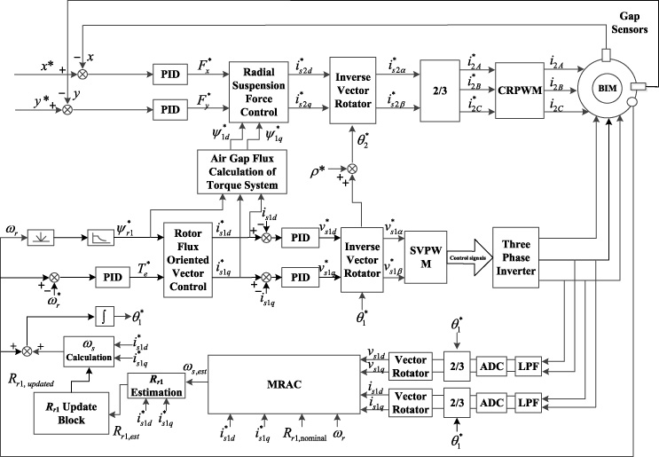
Block diagram of the MRAC-based rotor resistance estimation for IFOC BIM drive.

3.2. Theoretical development of the proposed scheme

BIM is basically an induction motor. Referring to synchronous rotating reference frame, the d and q-axis voltages of the rotating part of the BIM can be expressed as: $\begin{eqnarray}\displaystyle \text{v}_{s1d}=R_{s1}i_{s1d}+{\sigma}L_{s1}pi_{s1d}+{\displaystyle \frac{L_{m1}}{L_{r1}}}p{\psi}_{r1d}-{\sigma}L_{s1}{\omega}_{1}i_{s1q}-{\omega}_{1}{\displaystyle \frac{L_{m1}}{L_{r1}}}{\psi}_{r1q} & & \displaystyle\end{eqnarray}$ (1) $\begin{eqnarray}\displaystyle \text{v}_{s1q}=R_{s1}i_{s1q}+{\sigma}L_{s1}pi_{s1q}+{\displaystyle \frac{L_{m1}}{L_{r1}}}p{\psi}_{r1q}+{\sigma}L_{s1}{\omega}_{1}i_{s1d}+{\omega}_{1}{\displaystyle \frac{L_{m1}}{L_{r1}}}{\psi}_{r1d}, & & \displaystyle\end{eqnarray}$ (2) where “p” represents the (d∕dt) operator and ω₁ = ω_s + ω_r. The instantaneous reactive power of rotating part of the BIM (Q) can be expressed as $\begin{eqnarray}\displaystyle Q_{1}=v_{s1q}i_{s1d}-v_{s1d}i_{s1q} & & \displaystyle\end{eqnarray}$ (3) Combining (1) and (2) in (3), the new presentation of Q is $\begin{eqnarray}\displaystyle Q_{2} & = & \displaystyle {\sigma}L_{s1}\left(pi_{s1q}i_{s1d}-pi_{s1d}i_{s1q}\right)+{\sigma}L_{s1}{\omega}_{1}(i_{s1d}^{2}+i_{s1q}^{2})\nonumber\\ \displaystyle \text{} & \text{} & \displaystyle -∼{\displaystyle \frac{L_{m1}}{L_{r1}}}(p{\psi}_{r1d}i_{s1q}-p{\psi}_{r1q}i_{s1d})+{\omega}_{1}{\displaystyle \frac{L_{m1}}{L_{r1}}}({\psi}_{r1q}i_{s1q}+{\psi}_{r1d}i_{s1d}).\end{eqnarray}$ (4)

Identification of the stator resistance is not required to be a significant feature of the above reactive power model. It is a remarkable feature of any reactive power-based model.

In the steady state, the derivative term is zero. Thus, the expression of Q simplifies to $\begin{eqnarray}\displaystyle Q_{3}={\sigma}L_{s1}{\omega}_{1}(i_{s1d}^{2}+i_{s1q}^{2})+{\omega}_{1}{\displaystyle \frac{L_{m1}}{L_{r1}}}({\psi}_{r1q}i_{s1q}+{\psi}_{r1d}i_{s1d}). & & \displaystyle\end{eqnarray}$ (5)

Adding the condition 𝜓_r1d = L _m1 i _s1d and 𝜓_r1q = 0 to (5) for indirect field-oriented control (IFOC) of BIM, the more simplified expression of Q is $\begin{eqnarray}\displaystyle Q_{4}={\sigma}L_{s1}{\omega}_{1}(i_{s1d}^{2}+i_{s1q}^{2})+{\omega}_{1}\frac{L_{m1}^{2}}{L_{r1}}i_{s1d}^{2}. & & \displaystyle\end{eqnarray}$ (6)

Since Q ₁ is independent of slid-speed term, it is chosen as the reference model consistently from the above expressions of Q. In the remaining expressions Q (such as, Q ₂, Q ₃ and Q ₄), Q ₄ is used in the adjustable model because it is dependent on slid speed. In addition, Q ₄ is independent of rotor fluxes and several derivative terms.

Fig. 4.

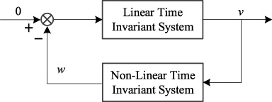
Nonlinear feedback system.

3.3. Stability of the proposed MRAC

As shown in Fig. 4, the design of MRAC is determined by the concept of Hyperstability [53]. The MARC mainly concerns the stability characteristics of ordinary feedback systems. If the system satisfies following two conditions, the feedback system will be globally stable.

Ensure that the transfer function of the linear stationary block is a strictly positive real function.

The nonlinear feedback block satisfies the Popov’s integral inequality $\begin{eqnarray}\displaystyle {\eta}(0,t_{1})=\int _{0}^{t_{1}}v^{T}wdt\geq -{\gamma}^{2}\quad \forall t_{1}>0 & & \displaystyle\end{eqnarray}$ (7) where 𝜈 is the input vector, w is the output vector of the feedback block, and 𝛾² is a finite positive constant.

Formation of the equivalent MRAC is shown in Fig. 5. Reference model and Adjustable model are as follow $\begin{eqnarray}\displaystyle \text{} & \text{} & \displaystyle Q_{ref}=v_{s1q}i_{s1d}-v_{s1d}i_{s1q}\end{eqnarray}$ (8) $\begin{eqnarray}\displaystyle \text{} & \text{} & \displaystyle Q_{est}={\sigma}L_{s1}{\omega}_{1}(i_{s1d}^{2}+i_{s1q}^{2})+{\omega}_{1}{\displaystyle \frac{L_{m1}^{2}}{L_{r1}}}i_{s1d}^{2}.\end{eqnarray}$ (9)

Subtracting (8) from (7) $\begin{eqnarray}\displaystyle Q_{ref}-Q_{est} & = & \displaystyle (v_{s1q}i_{s1d}-v_{s1d}i_{s1q})\nonumber\\ \displaystyle \text{} & \text{} & \displaystyle -∼{\omega}_{1}({\varepsilon},t)\left\{{\sigma}L_{s1}(i_{s1d}^{2}+i_{s1q}^{2})+(L_{m1}^{2}/L_{r1})i_{s1d}^{2}\right\}.\nonumber\end{eqnarray}$

As can be seen from the structure of Fig. 2, ω₁(ϵ, t) = ω_{s, nom} + δω_{s, est}(ϵ, t) + ω_r. Therefore $\begin{eqnarray}\displaystyle {\varepsilon}={\rho}_{1}-\left\{{\omega}_{s,nom}+{\delta}{\omega}_{s,est}\left({\varepsilon},t\right)+{\omega}_{r}\right\}{\rho}_{2}, & & \displaystyle\end{eqnarray}$ (10) where 𝜌₁ = v _s1q i _s1d − v _s1d i _s1q and ${\rho}_{2}={\sigma}L_{s1}(i_{s1d}^{2}+i_{s1q}^{2})+\frac{L_{m1}^{2}}{L_{r}}i_{s1d}^{2}$ . Considering to the general structure of the adaptation law, the δω_{s, est} (ϵ, t) will be presented for the concrete form of expression $\begin{eqnarray}\displaystyle {\delta}{\omega}_{s,est}({\varepsilon},t)=\left(k_{p}+{\displaystyle \frac{k_{I}}{s}}\right)v & & \displaystyle\end{eqnarray}$ (11) where 𝜈 is the output of a block D and used to adjust error function, D is usually taken as unit matrix $\begin{eqnarray}\displaystyle v=D\cdot {\varepsilon}={\varepsilon}. & & \displaystyle\end{eqnarray}$ (12)

According to Fig. 5, make $\begin{eqnarray}\displaystyle u={\rho}_{1}-\{{\omega}_{s,nom}+{\delta}{\omega}_{s,est}({\varepsilon},t)+{\omega}_{r}\}{\rho}_{2}. & & \displaystyle\end{eqnarray}$ (13)

Thus, according to (10), ϵ = u can be obtained. It is assumed that w = −u $\begin{eqnarray}\displaystyle w=-u=-{\rho}_{1}+\{{\omega}_{s,nom}+{\delta}{\omega}_{s,est}({\varepsilon},t)+{\omega}_{r}\}{\rho}_{2}. & & \displaystyle\end{eqnarray}$ (14)

Substituting ω and v from (12) and (14) into (7), the formula can be simplified to $\begin{eqnarray}\displaystyle \int _{0}^{t1}\left\{-v{\rho}_{1}+{\omega}_{s}v{\rho}_{2}+\left(k_{P}+{\displaystyle \frac{k_{I}}{s}}\right)v^{2}{\rho}_{2}+{\omega}_{r}v{\rho}_{2}\right\}dt\geq -{\gamma}^{2}. & & \displaystyle\end{eqnarray}$ (15)

According to the following famous inequality, it can be demonstrated that the inequality (15) is satisfied: $\begin{eqnarray}\displaystyle \int _{0}^{t1}\frac{d}{dt}f(t)k_{1}f(t)dt\geq -{\displaystyle \frac{1}{2}}k_{1}f(0)^{2}\quad \forall k_{1}>0. & & \displaystyle\end{eqnarray}$ (16)

Thus, Popov’s integral inequality is satisfied completely by the PI controller. The other condition that needs to be met is to make the transfer function of the feedforward linear stationary block positive. To meet this, the error manipulation block “D” is included in Fig. 5, which achieves the same by properly setting the sign of ϵ. These make the Popov’s criterion satisfied and the stability of the system is proved.

Fig. 5.

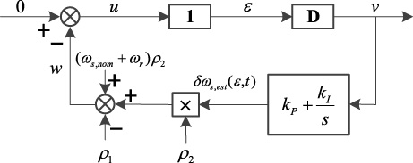
Equivalent nonlinear feedback scheme.

Fig. 6.

Step response of rotor sensitivity function and stator sensitivity function.

3.4. Sensitivity analysis of the proposed MRAC

(1) Sensitivity to rotor resistance: The rotating part of the BIM regarding to synchronous coordinate system model at steady state can be expressed as: $\begin{eqnarray}\displaystyle \text{} & \text{} & \displaystyle \frac{d}{dt}\left[\begin{array}{@{}c@{}}i_{s1}\\ {\psi}_{r1}\end{array}\right]=\left[\begin{array}{@{}cc@{}}-(a_{1}I+{\omega}_{1}J) & a_{2}I-a_{3}{\omega}_{r}J\\ a_{4}I & -(a_{5}I+{\omega}_{s}J)\end{array}\right]\left[\begin{array}{@{}c@{}}i_{s1}\\ {\psi}_{r1}\end{array}\right]+\left[\begin{array}{@{}cc@{}}I & 0\\ 0 & 0\end{array}\right]v_{s1}\end{eqnarray}$ (17) $\begin{eqnarray}\displaystyle \text{} & \text{} & \displaystyle i_{s1}=\left[\begin{array}{@{}cc@{}}I & 0\end{array}\right]\left[\begin{array}{@{}c@{}}i_{s1}\\ {\psi}_{r1}\end{array}\right],\end{eqnarray}$ (18) where $a_{1}=\frac{1}{{\sigma}L_{s1}}\left(R_{s1}+\frac{L_{m1}^{2}}{L_{r1}T_{r1}}\right)$ , $a_{2}=\frac{1}{{\sigma}L_{s1}}\left(\frac{L_{m1}}{L_{r1}T_{r1}}\right)$ , $a_{3}=\frac{1}{{\sigma}L_{s1}}\left(\frac{L_{m1}}{L_{r1}}\right)$ , $a_{4}=\frac{L_{m1}}{T_{r1}}$ , $a_{5}=\frac{1}{T_{r1}}$ , $I=\left[\begin{array}{@{}cc@{}}1 & 0\\ 0 & 1\end{array}\right]$ and $J=\left[\begin{array}{@{}cc@{}}0 & -1\\ 1 & 0\end{array}\right]$ . Equation ((18)) can be expressed to $\begin{eqnarray}\displaystyle {\dot{x}}=Ax+Bu. & & \displaystyle\end{eqnarray}$ (19)

After linearization regarding with the working point (x), the small signal model of (19) can be expressed as $\begin{eqnarray}\displaystyle \text{} & \text{} & \displaystyle {\Delta}{\dot{x}}=A{\Delta}x+{\Delta}Ax\end{eqnarray}$ (20) $\begin{eqnarray}\displaystyle \text{} & \text{} & \displaystyle {\Delta}i_{s1}=C{\Delta}x.\end{eqnarray}$ (21)

Thus, $\begin{eqnarray}\displaystyle {\Delta}i_{s1}(s)=C(sI-A)^{-1}{\Delta}A(s)x, & & \displaystyle\end{eqnarray}$ (22) where $\begin{eqnarray}\displaystyle {\Delta}A=\left[\begin{array}{@{}cc@{}}b_{1}I & -b_{2}I\\ -b_{3}I & b_{4}I\end{array}\right]{\Delta}R_{r1}. & & \displaystyle\end{eqnarray}$ (23) Here, $b_{1}=\frac{1}{{\sigma}L_{s1}}\left(\frac{L_{m1}^{2}}{L_{r1}^{2}}\right)$ , $b_{2}=\frac{1}{{\sigma}L_{s1}}\left(\frac{L_{m1}}{L_{r1}^{2}}\right)$ , $b_{3}=\frac{L_{m1}}{L_{r1}}$ , $b_{4}=\frac{1}{L_{r1}}$ . The expression of (Δi _s ₁∕ΔR _r1) can be given by substituting ((23)) into ((22)). After linearization regarding with the operating point, (Δω_s∕Δi _s1) can be obtained from the small signal model of ((11)). Now, the sensitivity function of the rotor change can be obtained for the proposed MRAC. $\begin{eqnarray}\displaystyle \frac{{\Delta}{\omega}_{s}}{{\Delta}R_{r1}}=\frac{(v_{s1q}-2k_{1}{\omega}_{1}i_{s1d})\frac{{\Delta}i_{s1d}}{{\Delta}R_{r1}}-(v_{s1d}+2{\sigma}L_{s1}{\omega}_{1}i_{s1q})\frac{{\Delta}i_{s1q}}{{\Delta}R_{r1}}}{(k_{1}i_{s1d}^{2}+{\sigma}L_{s1}i_{s1q}^{2})+\left(k_{p}+\frac{k_{I}}{s}\right)^{-1}} & & \displaystyle\end{eqnarray}$ (24) where $k_{1}={\sigma}L_{s1}+\frac{L_{m1}^{2}}{L_{r1}}$ and K _P, K _I can be got from the PI controller that satisfies the adaptation law. As is shown in Fig. 6, the step response of the sensitivity function is presented in ((24)). The response indicates that any changes can be estimated by correctly identifying the slip speed.

(2) Sensitivity to stator resistance: The matrix ΔA can be expressed as (25) after a small change in R _s1 $\begin{eqnarray}\displaystyle {\Delta}A=\left[\begin{array}{@{}cc@{}}\frac{1}{{\sigma}L_{s1}}I & 0\\ 0 & 0\end{array}\right]{\Delta}R_{s1}. & & \displaystyle\end{eqnarray}$ (25)

As the same with the sensitivity function of the rotor resistance, the sensitivity function of the stator resistance ( $Δω_s = ΔR_{s1}$ ) can also be obtained. Figure 6 shows the step response of the sensitivity function. This can be included that the estimation mechanism at steady state is not affected by any change in stator resistance.

4. Vector control

For the control of the radial suspension force in the BIM, the distribution of the combined magnetic field in the air gap can be changed by adjusting the current of the suspension force windings, so that the magnitude and direction of the Maxwell force on the rotating shaft can be controlled, and finally the shaft suspension is achieved. Referring to synchronous rotating reference frame, radial suspension forces F _x and F _y can be expressed as: $\begin{eqnarray}\displaystyle \left\{\begin{array}{@{}l@{}}F_{x}=(K_{m}+K_{l})(i_{s2d}{\psi}_{1d}+i_{s2q}{\psi}_{1q})\\[6.0pt] F_{y}=(K_{m}+K_{l})(i_{s2q}{\psi}_{1d}-i_{s2d}{\psi}_{1q})\end{array}\right. & & \displaystyle\end{eqnarray}$ (26) where $K_{l}=\frac{p_{1}W_{2}}{2rW_{1}}$ and $K_{m}=\frac{{\pi}p_{1}p_{2}L_{m2}}{18{\mu}_{0}lrW_{1}W_{2}}$ are the Lorentz forces constant and Maxwell forces constant respectively, the d and q-axis components of air-gap flux of torque windings are expressed by 𝜓_1d and 𝜓_1q respectively, the d and q-axis components of stator current of suspension force windings are expressed by i _s2d and i _s2q respectively, the mutual inductance of suspension force windings is expressed by L _m2, the number of pole pairs of torque windings and suspension force windings is expressed by p ₁ and p ₂, the number of turns of torque windings and suspension force windings is expressed by W ₁ and W ₂, respectively, the radius of the stator inner surface is expressed by r, and 𝜇₀ express the vacuum permeability.

Table 1

Parameters of BIM

Parameter	Value
L _s1	16.514 × 10⁻² H
L _r1	16.509 × 10⁻² H
L _m1	16.081 × 10⁻² H
R _s1	0.877Ω
R _r1	1.48Ω
J	0.015 kg ⋅ m⁻²
p ₁	2
p ₂	1

For realizing stable suspension and operation of the BIM, the realization of nonlinear decoupling control between electromagnetic torque and radial suspension forces is the basic requirement. Many reliable methods can be applied to achieve it, and vector control is one of them. Regarding to the vector control (In this paper, vector control is represented by indirect rotor flux-oriented control), the rotor magnetic field of the torque windings is defined on the same axis as the d-axis of the rotating coordinate axis, which means 𝜓_r1d = L _m1 i _s1d and 𝜓_r1q = 0. Then, the currents of torque windings i _s1d and i _s1q, the electromagnetic torque T _e and slip angular speed ω_s can be expressed as $\begin{eqnarray}\displaystyle \left\{\begin{array}{@{}l@{}}i_{s1d}=(T_{r1}p_{1}{\psi}_{r1}+{\psi}_{r1})/L_{m1}\\[6.0pt] i_{s1q}=T_{e}L_{r1}/(p_{1}{\psi}_{r1}L_{m1})\\[6.0pt] {\omega}_{s}={\omega}_{1}-{\omega}_{r}=i_{s1q}L_{m1}/({\psi}_{r1}T_{r1})\\[6.0pt] T_{e}={\psi}_{r1}i_{s1q}L_{m1}p_{1}/L_{r1}.\end{array}\right. & & \displaystyle\end{eqnarray}$ (27)

From ((11)), it can be concluded that the radial suspension force is the result of the interaction between the air-gap flux of the torque windings and current of suspension control windings. Hence, to obtain excellent radial suspension forces, it is essential to obtain the air-gap flux. The relationship between the rotor flux linkage and the air gap flux linkage can be obtained when the BIM achieves rotor field orientation control. Air-gap flux can be got by calculating the rotor flux and stator current of torque windings. The specific formula can be expressed as: $\begin{eqnarray}\displaystyle \left\{\begin{array}{@{}l@{}}{\psi}_{1d}={\displaystyle \frac{L_{m1}}{L_{r1}}}\left({\psi}_{r1d}+L_{r1l}i_{s1d}\right)\\ {\psi}_{1q}={\displaystyle \frac{L_{m1}}{L_{r1}}}L_{r1l}i_{s1q}.\end{array}\right. & & \displaystyle\end{eqnarray}$ (28)

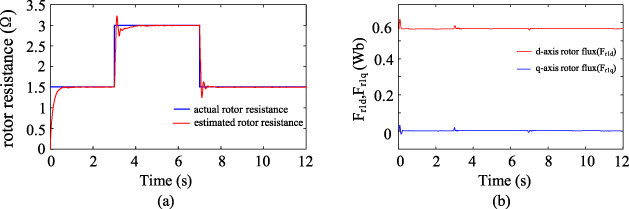
According to the suspension force formula ((26)), once the air gap flux value is obtained, the current value required for the suspension control windings can also be obtained by ((29)) $\begin{eqnarray}\displaystyle \left[\begin{array}{@{}c@{}}i_{s2d}\\ i_{s2q}\end{array}\right]={\displaystyle \frac{1}{M}}\left[\begin{array}{@{}cc@{}}\cos {\rho} & -\sin {\rho}\\ \sin {\rho} & \cos {\rho}\end{array}\right]\left[\begin{array}{@{}c@{}}F_{x}\\ F_{y}\end{array}\right] & & \displaystyle\end{eqnarray}$ (29) where ${\rho}=\arctan (\frac{{\psi}_{1q}}{{\psi}_{1d}})$ and $M=(K_{m}+K_{l})\sqrt{{\psi}_{1d}^{2}+{\psi}_{1q}^{2}}.$

Fig. 7.

Step change in rotor resistance: (a) actual rotor resistance and estimated rotor resistance, (b) d and q-axis flux.

Fig. 8.

Rotor resistance estimation at zero speed: (a) actual and estimated rotor resistance with step change in stator resistance, (b) d and q-axis rotor flux.

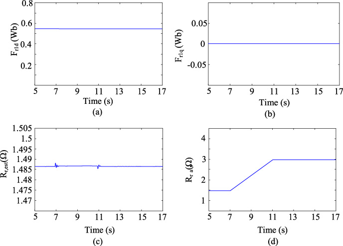
Figure 2 shows the block diagram of MRAC-based rotor resistance estimation for IFO BIM drive. For the radial suspension force control subsystem, the deviation between the rotor radial displacement detected by displacement sensor and reference values x ^∗ and y ^∗ generates the radial suspension force commands $F_{x}^{\ast }$ and $F_{y}^{\ast }$ by proportional–integral–derivative controllers. Then, current commands $i_{s2d}^{\ast }$ and $i_{s2q}^{\ast }$ for the suspension force windings can be got by (29). These commands are modulated by inverse Park transformation and 2/3 transformation. Then, it generates suspension force windings current commands $i_{2A}^{\ast }$ , $i_{2B}^{\ast }$ , $i_{2C}^{\ast }$ . The current commands $i_{2A}^{\ast }$ , $i_{2B}^{\ast }$ , $i_{2C}^{\ast }$ are used to regulate currents of suspension force windings i _2A, i _2B, i _2C by a current-regulated pulse width modulation (CRPWM)-based inverter. Eventually, radial suspension force can be got in BIM.

Fig. 9.

Simulated result for slow variation in rotor resistance: (a) d-axis rotor flux, (b) q-axis rotor flux, (c) estimated rotor resistance, and (d) assumed rotor resistance.

For the torque control subsystem, the rotor speed ω_r detected by the photoelectric encoder is transformed to rotor flux-linkage command ${\Psi}_{r1}^{\ast }$ by flux generator and value ab-soluting. The deviation between detected rotor speed and given speed generates electromagnetic torque command $T_{e}^{\ast }$ by proportional–integral–derivative controllers. Then, torque windings current commands $i_{s1d}^{\ast }$ and $i_{s1q}^{\ast }$ can be got by rotor flux-oriented vector controller. These commands are compared with actual current commands. The errors are amplified by PID controllers to obtain reference voltage commands $v_{s1d}^{\ast }$ and $v_{s1q}^{\ast }$ . The slip angular speed ω_s got by MRAC in Fig. 1 is added to the detected rotating speed ω_r of the rotor and their sum is used as the synchronous rotating speed ω₁ of the torque windings and the suspension force windings, and the integral is obtained as the rotational transformation angle ${\theta}_{1}^{\ast }$ . ${\theta}_{2}^{\ast }$ is determined by the rotational transformation angle ${\theta}_{1}^{\ast }$ and compensation angle 𝜌∗. ${\theta}_{1}^{\ast }$ and ${\theta}_{2}^{\ast }$ are used in the inverse Park transformation and the orientation of the obtained flux will be more accurate. $v_{s1a}^{\ast }$ and $v_{s1b}^{\ast }$ got by the inverse Park transformation drive the three-phase inverter to control the BIM through the regulation of SVPWM.

Fig. 10.

Vector controlled BIM drive with MRAC-based speed estimator.

5. Simulation results

To verify the feasibility of the proposed MRAC-based rotor resistance estimation scheme. MATLAB/SIMULINK was used to simulate the IFO-controlled BIM driver. The BIM parameters and rating are given in Table 1.

Fig. 11.

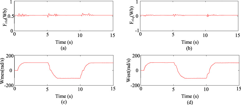
Simulated results for speed reversal: (a) d-axis rotor flux, (b) q-axis rotor flux, (c) actual rotor speed, and (d) estimated rotor speed.

Figure 7 shows the curves of the actual and estimated rotor resistance, and d and q-axis rotor flux with step change in rotor resistance. Of course, in actual driving, the rotor resistance changes with the operating temperature, but the rotor resistance does not change suddenly because the large thermal time constant. The step change of the rotor resistance represents an extreme situation, and based on this case, the robustness of the proposed MRAC can be displayed.

The simulated results of the rotor resistance estimation are shown in the Fig. 8 at the zero speed. As it is shown in Fig. 8(a), the stator resistance exerts a step change at 7s. The rotor resistance estimation is not influenced by the step change in stator resistance. The d and q-axis rotor flux are shown in Fig. 8(b).

Fig. 12.

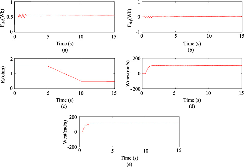
Simulated results for speed estimation under change in rotor resistance (from Rr to 0.5 Rr): (a) d-axis rotor flx, (b) q-axis rotor flux, (c) rotor resistance variation from Rr to 0.5 Rr, (d) actual rotor speed, and (e) estimated rotor speed.

In the actual system, the rotor resistance changes so slowly over time that it is difficult to be observed, it is impossible to capture their data over a long-time range. So in order to simulate the difference between the actual rotor resistance value and the controller value, it is assumed that the controller value varies in 7s and 11s, as shown in Fig. 9(d). However, MRAC identifies that their values of output are not equal, and makes the output values of the reference model and the adjustable model same by driving the PI controller, and the measured actual value of rotor resistance is shown in Fig. 9(c). Figure 9(a) and (b) show the curves of the corresponding d and q-axis rotor fluxes respectively.

6. Rotor resistance estimation in speed sensorless controller

Due to the speed sensorless controller mentioned in several literatures [54–57] on rotor resistance estimation, the attempted scheme is proposed. The section describes how to modify MRAC to achieve a speed sensorless controller together with online rotor resistance estimation. Figure 10 shows relevant MRAC-based speed estimator. Now flux estimation is demanded by the current system. In addition, flux tuning controller is also known as the PI controller. It is used for the orientation of flux. The stability of the entire system is verified by Popov’s Hyper Stability Criterion. The whole process is the same as the rotor resistance estimation in Section 4.3.

The proposed MRAC-based speed estimator is used to test by giving a step change in command speed. The command speed is set to 100 rad/s at 0.5 seconds and is maintained for 4.5 seconds. At 5 seconds, the command speed is set to a negative speed command for −100 rad/s. At last, set the speed command to 100 rad/s again at 10 seconds. Figure 11 shows simulated result curves of d-axis and q-axis flux, the actual rotor speed and the estimated speed. It can be seen from the simulated results that the system can work stably regardless of whether the forward rotor speed command or the reverse rotor speed command is set.

Eventually, another simulated result is shown in Fig. 12. It shows that the controller can maintain the orientation of flux after the variation of rotor resistance. In this simulation, the rotor resistance is changed from R _r to 0.5R _r slowly in 5s. Therefore, this simulation shows that the speed estimation is not affected by parameter of rotor resistance. Figures 12(c) and (d) show the estimated speed and actual speed, respectively. Figure 12(a) and (b) show the d-axis and q-axis rotor flux.

7. Conclusion

This paper presents the detailed performance of rotor resistance estimation technique based on MRAC of the BIM. The instantaneous reactive power and steady-state reactive power of the rotating part of the BIM is selected in the MRAC as reference model and adjustable model. This selection of model has the following advantages.

It is not influenced by the stator resistance.

The calculation of the flux linkage is not required, so it is independent of the integration.

There is no derivative term in the MRAC model, hence it is free from noise-related problems.

Reference model is completely immune to machine parameters

The calculation process of the entire reference model and adjustable model is relatively simple.

The speed sensorless scheme is proposed after adding the flux estimation. At last, speed sensorless technique can be achieved together with online rotor resistance estimation. The proposed scheme is simulated in MATLAB/SIMULINK. The feasibility of the scheme is also validated by the simulated results.

Footnotes

Acknowledgements

This work was supported by the National Natural Science Foundation of China under Projects 51875261 and 51475214, the Natural Science Foundation of Jiangsu Province of China under Projects BK20180046 and BK20170071, the “Qinglan project” of Jiangsu Province, the Key Project of Natural Science Foundation of Jiangsu Higher Education Institutions under Project 17KJA460005, the Six Categories Talent Peak of Jiangsu Province under Projects2016-GDZB-096 and 2015-XNYQC-003, and the “333 project” of Jiangsu Province under Project BRA2017441.

References

Sun

Chen

and Yang

, Overview of bearingless permanent magnet synchronous motors, IEEE Transactions on Industrial Electronics 60(12) (2013), 5528–5538.

Sinervo

and Arkkio

, Rotor radial position control and its effect on the total efficiency of a bearingless induction motor with a cage rotor, IEEE Transactions on Magnetics 50(4) (2014), 1–9.

Grabner

Amrhein

Silber

and Gruber

, Nonlinear feedback control of a bearingless brushless DC motor, IEEE/ASME Transactions on Mechatronics 15(1) (2010), 40–47.

Grabner

Amrhein

Silber

and Gruber

, Nonlinear feedback control of a bearingless brushless DC motor, IEEE Transactions on Mechatronics 15(1) (2010), 40–47.

Chiba

Fukao

and Rahman

M.A.

, Vibration suppression of a flexible shaft with a simplified bearingless induction motor drive, IEEE Transactions on Industry Applications 44(3) (2008), 745–752.

Sun

Shi

Chen

and Yang

, Internal model control for a bearingless permanent magnet synchronous motor based on inverse system method, IEEE Transactions on Energy Conversion 31(4) (2016), 1539–1548.

Sun

Lei

Guo

and Zhu

, State feedback control for a PM hub motor based on grey wolf optimization algorithm, IEEE Transactions on Power Electronics (2019), doi:10.1109/TPEL.2019.2923726.

Sun

Diao

Lei

Guo

and Zhu

, Study on segmented-rotor switched reluctance motors with different rotor pole numbers for BSG system of hybrid electric vehicles, IEEE Transactions on Vehicular Technology 68(6) (2019), 5537–5547.

Sun

Shen

Wang

Lei

Yang

and Han

, Core losses analysis of a novel 16/10 segmented rotor switched reluctance BSG motor for HEVs using nonlinear lumped parameter equivalent circuit model, IEEE/ASME Transactions on Mechatronics 23(2) (2018), 747–757.

10.

Sun

Diao

and Yang

, Performance improvement of a switched reluctance machine with segmental rotors for hybrid electric vehicles, Computers and Electrical Engineering (2019), 244–259.

11.

Sun

Jin

and Yang

, Performance improvement of torque and suspension force for a novel five-phase BFSPM machine for flywheel energy storage systems, IEEE Transactions on Applied Superconductivity 29(2) (2019), 0601505.

12.

Cheng

Sun

and Yang

, A nonlinear flux linkage model for bearingless induction motor based on GWO-LSSVM, IEEE Access 7 (2019), 36558–36567.

13.

Sun

Xue

and Zhu

, Suspension force modeling for a bearingless permanent magnet synchronous motor using maxwell stress tensor method, IEEE Transactions on Applied Superconductivity 26(7) (2016), 0608705.

14.

Hiromi

Katou

Chiba

Rahman

M.A.

and Fukao

, A novel magnetic suspension-force compensation in bearingless induction-motor drive with squirrel-cage rotor, IEEE Transactions on Industry Applications 43(1) (2007), 66–76.

15.

Chiba

and Santisteban

J.A.

, A PWM harmonics elimination method in simultaneous estimation of magnetic field and displacements in bearingless induction motors, IEEE Transactions on Industry Applications 48(1) (2012), 124–131.

16.

Choi

and Gweon

, A high-precision dual-servo stage using halbach linear active magnetic bearings, IEEE/ASME Transactions on Mechatronics 16(5) (2011), 925–931.

17.

Yan

Hsu

Wang

Tsai

and Wu

, Axial-flux permanent magnet brushless motor for slim vortex pumps, IEEE Transactions on Magnetics 45(10) (2009), 4732–4735.

18.

Noh

Gruber

and Trumper

D.L.

, Hysteresis bearingless slice motors with homopolar flux-biasing, IEEE/ASME Transactions on Mechatronics 22(5) (2017), 2308–2318.

19.

Belahcen

Mukhrejee

Martin

and Rasilo

, Computation of hysteresis torque and losses in a bearingless synchronous reluctance machine, IEEE Transactions on Magnetics 54(3) (2018), 1–4.

20.

Yang

and Zhang

, Modelling and performance analysis on a bearingless fixed-pole rotor induction motor, IET Electric Power Applications 13(2) (2019), 251–258.

21.

Sun

Wang

Yang

Lei

Zhu

and Guo

, Performance analysis of suspension force and torque in an IBPMSM with V-shaped PMs for flywheel batteries, IEEE Transactions on Magnetics 54(11) (2018), 8105504.

22.

Tera

Yamauchi

Chiba

Fukao

and Rahman

M.A.

, Performances of bearingless and sensorless induction motor drive based on mutual inductances and rotor displacements estimation, IEEE Transactions on Industrial Electronics 53(1) (2006), 187–194.

23.

Sugimoto

Miyoshi

and Chiba

, Axial vibration suppression by field flux regulation in two-axis actively positioned permanent magnet bearingless motors with axial position estimation, IEEE Transactions on Industry Applications 54(2) (2018), 1264–1272.

24.

Jabbour

and Mademlis

, Online parameters estimation and autotuning of a discrete time model predictive speed controller for induction motor drives, IEEE Transactions on Power Electronics 34(2) (2019), 1548–1559.

25.

Zhang

and Xiao

, Inverse system decoupling control strategy of BLIM based on stator flux orientation, International Journal of Applied Electromagnetics and Mechanics 48(4) (2015), 469–480.

26.

Cheng

Qiao

Zhang

and Xu

, Inverse system modeling and decoupling control of bearingless induction motor based on air gap flux orientation, International Journal of Applied Electromagnetics and Mechanics 53(3) (2017), 567–577.

27.

and Xiao

, Unbalanced vibration control strategy of bearingless induction motor based on inverse system decoupling, International Journal of Applied Electromagnetics and Mechanics 51(4) (2016), 455–469.

28.

Wang

and Liu

, An improved rotor flux-oriented control system of bearingless induction motors, in: Chinese Control and Decision Conference, Xuzhou, 2010, pp. 2733–2737.

29.

Shi

Sun

Cai

Yang

Lei

Guo

and Zhu

, Torque analysis and dynamic performance improvement of A PMSM for EVs by skew angle optimization, IEEE Transactions on Applied Superconductivity 29(2) (2019), 0600305.

30.

Sun

Zhu

Wang

Zhou

Yang

Lei

Zhu

and Guo

, MPTC for PMSMs of EVs with multi-motor driven system considering optimal energy allocation, IEEE Transactions on Magnetics 55(7) (2019), 8104306.

31.

Sun

Chen

Yang

and Zhu

, Speed-sensorless vector control of a bearingless induction motor with articial neural network inverse speed observer, IEEE/ASME Transactions on Mechatronics 18(4) (2013), 1357–1366.

32.

Sun

Chen

Yang

and Shi

, Precise control of a four degree-of-freedom permanent magnet biased active magnetic bearing system in a magnetically suspended direct-driven spindle using neural network inverse scheme, Mechanical Systems and Signal Processing 88 (2017), 36–48.

33.

Reigosa

D.D.

Briz

Blanco

and Guerrero

J.M.

, Sensorless control of doubly fed induction generators based on stator high-frequency signal injection, IEEE Transactions on Industry Applications 50(5) (2014), 3382–3391.

34.

Chiba

Sotome

Iiyama

and Rahman

M.A.

, A novel middle point current injection type bearingless PM synchronous motor for vibration suppression, IEEE Transactions on Industry Applications 47(4) (2011), 1700–1706.

35.

Liu

Wang

Cao

and Wang

, Speed-sensorless direct torque control of bearingless permanent magnet synchronous motor based on extended Kalman filter, in: International Conference on Measuring Technology and Mechatronics Automation, Changsha, 2010, pp. 457–460.

36.

Pal

Das

and Chattopadhyay

A.K.

, An improved rotor flux space vector based MRAS for field-oriented control of induction motor drives, IEEE Transactions on Power Electronics 33(6) (2018), 5131–5141.

37.

Cao

Zhang

Yang

Xie

and Zhang

, Reactive-power-based MRAS for online rotor time constant estimation in induction motor drives, IEEE Transactions on Power Electronics 33(12) (2018), 10835–10845.

38.

Manohar

and Das

, Combined speed and rotor resistance estimation for speed sensorless induction motor drive using reactive power based MRAS, Michael Faraday IET International Summit (2015), 330–335.

39.

Ravi Teja

A.V.

Verma

and Chakraborty

, A new formulation of reactive power based model reference adaptive system for sensorless induction motor drive, IEEE Transactions on Industrial Electronics 62(11) (2015), 6797–6808.

40.

Cao

Zhang

Yang

Xie

and Zhang

, Torque based model reference adaptive system updating rotor time constant in induction motor drives, in: IEEE Transportation Electrification Conference and Expo, Asia-Pacific, Harbin, 2017, pp. 1–5.

41.

Sun

Chen

and Jiang

, High-performance control for a bearingless permanent magnet synchronous motor using neural network inverse scheme plus internal model controllers, IEEE Transactions on Industrial Electronics 63(6) (2016), 1–1.

42.

Han

Zhang

Qiu

and Wang

, Multivariate chaotic time series online prediction based on improved kernel recursive least squares algorithm, IEEE Transactions on Cybernetics 49(4) (2019), 1160–1172.

43.

Bijan

M.G.

Al-Badri

Pillay

and Angers

, Induction machine parameter range constraints in genetic algorithm based efficiency estimation techniques, IEEE Transactions on Industry Applications 54(5) (2018), 4186–4197.

44.

Huang

Zhang

and Shi

, Unbalanced displacement LMS extraction algorithm and vibration control of a bearingless induction motor, International Journal of Applied Electromagnetics and Mechanics 56(1) (2018), 35–47.

45.

Zhang

Qiao

and Zhang

, Equivalent two-phase mutual inductance model and measurement algorithm of three-phase bearingless motor, Transactions of the Institute of Measurement and Control 40(2) (2018), 630–639.

46.

Garces

L.J.

, Parameter adaption for the speed-controlled static ac drive with a squirrel-cage induction motor, IEEE Transactions on Industry Applications 16(2) (1980), 173–178.

47.

Huang

and Lu

, A novel on-line rotor resistance estimation method for vector controlled induction motor drive, International Power Electronics and Motion Control Conference (2004), 655–660.

48.

Nait Said

M.S.

and Benbouzid

M.E.H.

, Induction motors direct field oriented control with robust on-line tuning of rotor resistance, IEEE Transactions on Energy Conversion 14(4) (1999), 1038–1042.

49.

Sun

Shi

Wang

Chen

Yang

and Li

, Linearizing control of a permanent magnet linear synchronous motor with inverse system scheme plus an internal model controller, International Journal of Applied Electromagnetics and Mechanics 55(4) (2017), 523–534.

50.

Sun

Chen

Yang

Qiao

and Han

, A high-performance control scheme for reluctance type bearingless motors, International Journal of Applied Electromagnetics and Mechanics 53(3) (2017), 537–549.

51.

Sun

Shen

Zhou

Yang

and Chen

, Modeling and control of a bearingless permanent magnet synchronous motor, International Journal of Applied Electromagnetics and Mechanics 53(1) (2017), 151–165.

52.

Yang

Sun

Zhu

and Zhao

, Active disturbance rejection control for bearingless induction motor based on hyperbolic tangent tracking differentiator, IEEE Journal of Emerging and Selected Topics in Power Electronics (2019), doi:10.1109/JESTPE.2019.2923793.

53.

Landau

, Adaptive control—the model reference approach, IEEE Transactions on Systems Man and Cybernetics 14(1) (1984), 169–170.

54.

Sun

Yang

Sun

and Zhang

, Speed sensorless of a bearingless induction motor based on super-twisting-model reference adaptive system, in: 20th International Conference on Electrical Machines and Systems (ICEMS), Sydney, 2017, pp. 1–5.

55.

Sun

Mao

Liu

and Wang

, The SVM-DTC system of the bearingless induction motor based on model reference adaptive, in: Proceedings of the 30th Chinese Control Conference, Yantai, 2011, pp. 3565–3569.

56.

Das

Kumar

and Pal

, MRAS-based speed estimation of induction motor drive utilizing machines’ d- and q-circuit impedances, IEEE Transactions on Industrial Electronics 66(6) (2019), 4286–4295.

57.

Accetta

Cirrincione

Pucci

and Vitale

, Closed-loop mras speed observer for linear induction motor drives, IEEE Transactions on Industry Applications 51(3) (2015), 2279–2290.