Lightning return stroke electromagnetic field and energy at close distance by using 3D FDTD simulation

Abstract

In this paper, the lightning return stroke electromagnetic field at close distance is calculated by the way of transmission line (TL) model and full-wave three-dimensional electromagnetic field simulation software XFDTD, which is based on finite-difference time-domain (FDTD) method. The evolution of distributions of electric field and magnetic field are summarized in the study. Furthermore, the total electromagnetic field and major components are analyzed to clarify the electromagnetic hazard from lightning electromagnetic pulse (LEMP). Then the temporal and spatial distribution characteristic of Poynting vector of the electromagnetic environment is shown to expound the energy distribution of LEMP at close distance. The results based on the analyses of field strength and Poynting vector show that the distribution of electric field, magnetic field and Poynting vector at close distance is akin to multilayered cylinder, and LEMP in the region characterized by large amplitude, transient behavior and high electromagnetic energy is a potential threat to adjacent electronic equipments. Moreover, engineering basis concerning LEMP protection and electromagnetic compatibility (EMC) design in the region closed to the return stroke point can be provided by the synthetical analysis of LEMP.

Keywords

Lightning electromagnetic field return stroke Poynting vector

1. Introduction

In view of the lightning damage effect and electromagnetic hazard on electronic device and overhead power transmission line suffered from the strong LEMP during the process of lightning return stroke [1,2], it’s imperative to investigate the mechanism of lightning return stroke, and compute electromagnetic field in engineering application.

For the numerical calculation of lightning electromagnetic field, both lightning return stroke model and channel-base current model are essential. lightning return stroke model is a mathematical conception aimed to reproduce the physical processes in the lightning discharge, which includes gas dynamic models, electromagnetic models, distributed-circuit models and engineering models [3–7]. Considering that the TL model [3] is convenience to describe the propagation of lightning current, it is usually adopted as the lightning return stroke model. The base current models are also the important part of numerical simulation, including double exponential function model [6], Heidler function model [8], impulse function current model [9] and so on.

In addition, the precision of results of numerical simulation is also determined by the calculation method. The electromagnetic numerical calculation methods, which include the method of moments (MoM) [10], the finite-difference time-domain (FDTD) [11] method, the finite-element method (FEM) [12] and partial-element equivalent-circuit (PEEC) [13] method are most widely used to analyze electromagnetic fields and its effect in recent years. The propagation of electromagnetic waves in the space can be well simulated by the FDTD method involving the space and time discretization of the solution space and the finite-difference approximation to differential form of Maxwell's equations. This method considers the full-wave process and analyzes the current distribution and the synthetic electromagnetic field in the conductor system. Accordingly, the FDTD method is widely applied to the solution of lightning electromagnetic fields. In terms of distance scale, the researches about lightning electromagnetic field can be divided into two aspects. The researches at far distance [14–16] and the researches at close distance [17–23] mostly concentrate on the electromagnetic field itself or the electromagnetic effects.

In the light of the tasks of lightning electromagnetic field at close distance, scholars conduct the following representative researches. (1) the influence of constructions or other facilities to electromagnetic field [19,24], (2) the consideration of stratified conducting ground [22,25], (3) the condition of rough ground surface [17,20,26,27], (4) onefold calculation of electromagnetic field [18].

However, few researches is involved in the dynamic 3-D distribution [28] of lightning electromagnetic field. It’s worth noting that this research incorporates with the superiority of XFDTD. Compared with the numerical solution by programming code, the advantages of XFDTD include efficient modeling procedure, acceleration techniques of XStream, accurate solution for self-adapting division of FDTD cells and powerful ability of post-processing.

The purpose of this paper is to study the distribution of lightning return stroke electromagnetic field at close distance, which includes the dynamic 3-D distribution of field strength and electromagnetic energy at different cross sections, by the numerical simulation of lightning return stroke of cloud to ground (CG) flashes in XFDTD.

This paper is organized as follow: The method and computational models used in the XFDTD simulations are introduced in Section 2, and the distribution of electric field, magnetic field and Poynting vector in the region close to return stroke point is discussed in Section 3. The main conclusions are drawn in Section 4.

2. Method and computational models

2.1. The lightning electromagnetic field method

Uman [29] proposed a method for calculating the lightning electromagnetic field by Maxwell’s equations under condition of the vertical lightning channel current with finite length. In the simplified lightning return stroke model, which is comprised of the vertical lightning channel and the homogeneous, isotropic ground, that the temporal and spatial distribution of lightning current is specified makes it possible to realize the accurate calculation of electromagnetic field. In other words, the computation of return stroke electromagnetic field relies heavily on the distribution of lightning current that propagates upward along the longitudinal channel.

The components of electric and magnetic fields at P (r, 𝜙, z) can be calculated by the formula ((1)) ∼((3)) referred in [30,31]. The electromagnetic energy can be calculated by the formula (4), which denotes that the Poynting vector refers to the energy that flows through unit area perpendicularly. In the following expressions, the R represents the distance from the observation point to the position z ^′ , and r represents the horizontal distance from the observation point to the channel. The i (z ^′, t) is the current at arbitrary height z ^′ and arbitrary time t. The μ₀ is the permeability of vacuum. The σ₀ is the vacuum dielectric constant. And the c is the velocity of light. $\begin{eqnarray}\displaystyle E_{r}(r,{\varphi},z,t) & = & \displaystyle \frac{1}{4{\pi}{\varepsilon}_{0}}\left[\int _{-H}^{H}\frac{3r(z-z^{\prime })}{R^{5}}\int _{0}^{t}i(z^{\prime },{\tau}-R/c)d{\tau}dz^{\prime }\right.\nonumber\\ \displaystyle \text{} & \text{} & \displaystyle \left.+∼\int _{-H}^{H}\frac{3r(z-z^{\prime })}{cR^{4}}i(z^{\prime },{\tau}-R/c)dz^{\prime }-\int _{-H}^{H}\frac{r(z-z^{\prime })}{c^{2}R^{3}}\frac{\partial i(z^{\prime },{\tau}-R/c)}{\partial t}dz^{\prime }\right]\end{eqnarray}$ (1) $\begin{eqnarray}\displaystyle E_{z}(r,z,t) & = & \displaystyle \frac{1}{4{\pi}{\varepsilon}_{0}}\left[\int _{-H}^{H}\frac{2(z-z^{\prime })^{2}}{R^{5}}\int _{0}^{t}i(z^{\prime },{\tau}-R/c)d{\tau}dz^{\prime }\right.\nonumber\\ \displaystyle \text{} & \text{} & \displaystyle \left.+∼\int _{-H}^{H}\frac{2(z-z^{\prime })^{2}-r^{2}}{cR^{4}}i(z^{\prime },{\tau}-R/c)dz^{\prime }-\int _{-H}^{H}\frac{r(z-z^{\prime })}{c^{2}R^{3}}\frac{\partial i(z^{\prime },{\tau}-R/c)}{\partial t}dz^{\prime }\right]\end{eqnarray}$ (2) $\begin{eqnarray}\displaystyle \text{} & \text{} & \displaystyle H_{{\phi}}(r,z,t)=\frac{1}{4{\pi}}\left[\int _{-H}^{H}\frac{r}{R^{3}}i(z^{\prime },t-R/c)dz^{\prime }+\int _{-H}^{H}\frac{r}{cR^{2}}\frac{\partial i(z^{\prime },t-R/c)}{\partial t}dz^{\prime }\right]\end{eqnarray}$ (3) $\begin{eqnarray}\displaystyle \text{} & \text{} & \displaystyle S=E\times H.\end{eqnarray}$ (4)

In formula (1) ∼(2), the integral term including current i (z ^′, t) denotes the charges transferred by the differential element dz ^′, which is called the electrostatic field. This term is the dominant field component at close distance for its characteristic of strong distance dependance. The term including the derivative of the current is called radiation field, and the third term including the current induction field.

In formula (3), that the first term including current called induction field is the dominant field component close to the source. Moreover, the second term is called radiation field. It is noted that the lightning current plays an important role in the computation of the electromagnetic field. Considering that the engineering models have the advantage of a small number of control parameters, it allows to calculate the return stroke current at any position along the channel, and conveniently associates with a specific base current [32]. And the current expression of the engineering models [33] is given by following formula. $\begin{eqnarray}\displaystyle \begin{array}{@{}c@{}}i(z^{\prime },t)=u(t-z^{\prime }/v_{f})P(z^{\prime })i(0,t-z^{\prime }/v)\end{array} & & \displaystyle\end{eqnarray}$ (5) Where u (t) is the Heaviside function. P (z ^′) is the height-dependent current attenuation factor. i (0, t − z ^′∕v) is the base current. v _f is the return stroke speed. v is the propagation velocity of the current wave. In TL model, the current wave propagates along the channel is characterized by ideal transmission line without any distortion and attenuation, namely the parameters of P (z ^′) = 1 and v _f = v. And the current at the front of the channel is zero.

As for the base current, the combination of Double exponential function and Heidler function [5] is used to reproduce the measured base current owing to the validity of time derivative of Heidler function at t = 0 and the Double exponential function with the feature of adjusting the waveform by simple coefficients. And the expressions of composite function are shown as follow. $\begin{eqnarray}\displaystyle \text{} & \text{} & \displaystyle i(0,t)=\frac{I_{1}}{{\eta}}\frac{(t/{\tau}_{1})^{n}}{(1+(t/{\tau}_{1}))^{n}}e^{-t/{\tau}_{2}}+I_{2}(e^{-t/{\tau}_{3}}-e^{-t/{\tau}_{4}})\end{eqnarray}$ (6) $\begin{eqnarray}\displaystyle \text{} & \text{} & \displaystyle {\eta}=\exp [-({\tau}_{1}/{\tau}_{2})(n{\tau}_{2}/{\tau}_{1})^{1/n}].\end{eqnarray}$ (7)

In above formula, I ₁ and I ₂ are current peak. The 𝜂 is amplitude correction factor, which is described in formula ((7)). τ₁ and τ₃ are the rise constants. The τ₂ and τ₄ are the decay constants. The trend of current waveform is simultaneously determined by those four time constants. Besides, the value of exponent n is 2 in this paper.

2.2. 3D computational model in XFDTD

The 3D computational model, which is composed of lightning channel, lumped current source [34] and the ground, is simulated in XFDTD, taking into account the measured data, which is derived from the triggered-lightning experiments at Camp Blanding, Florida (1994) [35].

Fig. 1.

The schematic diagram of 3D simulation model in XFDTD.

2.2.1. 3D simulation model of lightning return stroke

The simulation model of CG return stroke in Cartesian coordinates is shown in Fig. 1. The return stroke channel is assumed to be perpendicular and straight, which is erected on the ground along the z-axis, so as to simulate the launching rocket trailing a thin grounded wire toward a charged cloud overhead in the triggered-lightning experiments. According to the details of the triggered-lightning experiments [36], the field enhancement near the rocket tip launches a positively charged leader that propagates upward toward the cloud, when the rocket, ascending at about 200 m/s, is about 200 to 300 m high. Based on the aforesaid details, the length of the channel is set to 2500 m in that the interest of the spatial dimension in this paper mainly concentrates on the lightning return stroke electromagnetic field within the atmospheric boundary layer. The conductivity and relative permittivity of the channel [37] are 10000 S/m, 5.3 respectively, which is related to the propagation speed of the current wave [38,39]. The image channel identical with the return stroke channel is embedded in the homogeneous and isotropic ground (1005 m × 1000 m × 2500 m) for the triggering site occupies a flat, open field with dimension of approximately 400 m by 700 m. Meanwhile, given the geographical conditions of Camp Blanding, Florida, USA located in 29°57^′25^′′ North, 81°59^′6^′′ West, much of the Florida’s surface is covered by a varying thickness of undifferentiated sediments consisting of siliciclastics, organics and carbonates, and its lithology characteristic appears as sedimentary rocks [40,41], so the ground characterized by conductivity of 0.01 S/m, relative permittivity of 10 and thickness of 2500 m [21] is similar to the real ground conditions, which induces field propagation effects. Furthermore, the return stroke current is transmitted to the channel and ground through the lumped current source.

2.2.2. The excitation source of the model

That the feed source(ideal current source), which expounds the specific channel-base current, is the critical part of the model associated with the accuracy of the calculation of the electromagnetic field. Therefore, formula (6) ∼(7) are utilized to reproduce the measured base current data of artificial triggered lightning [35]. The parameters of fitting current waveform is shown in Table 1. And the comparison of fitting current and the experimental current are depicted in Fig. 2.

Table 1
Parameters of fitting current waveform

I ₁/ (kA) I ₂/ (kA) τ₁∕μs τ₂∕μs τ₃∕μs τ₄∕μs

6.55 4.00 9.00 0.22 90.90 100.00

I ₁/ (kA)	I ₂/ (kA)	τ₁∕μs	τ₂∕μs	τ₃∕μs	τ₄∕μs
6.55	4.00	9.00	0.22	90.90	100.00

Fig. 2.

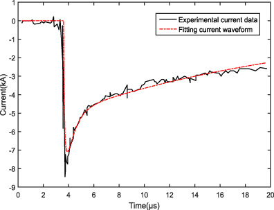
The comparison between the fitting current and the experimental current data.

The comparison of the current waveforms suggests that the rising and falling edges of the fitting curve can well reproduce the variation characteristics of base current waveform. Therefore, the fitting current waveform (from 3.6 μs to 18 μs) is chosen as the excitation source waveform. Except for the most important excitation source in the return stroke model, whether the numerical simulation results are consentaneous with measured electromagnetic fields data also hinges upon the configurations of FDTD numerical calculation.

2.2.3. Configuration of the FDTD calculation space

The cell size used to discretize the solution space should be compatible with the dimensions and features of the geometric structure of the target model, and it in turn will determine the runtime and memory costs of the simulation. The XFDTD can provide more accuracy in simulation results and optimized runtime by more than nonuniform grid type. In this paper, a nonuniform grid type is utilized to improve the effectiveness of simulation [42]. The cell size of the whole solution space (1005 m × 1000 m × 5000 m) is set to 9 m, and over-ground calculation space (105 m × 100 m × 100 m), which is adjacent to the return stroke point, is set to the FDTD cells with size of 5 m to research into the variation laws of lightning electromagnetic field in the horizontal direction. To further investigate the electromagnetic field at close distance, the cell size of solution space (105 m × 100 m × 5000 m) is set to 6 m, and over-ground calculation space (105 m × 100 m × 100 m) is set to 1 m to improve solving precision so that the distribution characteristics and change laws of field strength and electromagnetic energy at the close distance can be expounded. Moreover, the subcellular discretization of the computational domain is provided by XFDTD’s self-adaptive dividing of cell size. The gridding properties editor controls the placement of fixed points at automatically-determined locations on the part where one or more types of geometric features are detected. And the cell size of the region including channel is smaller than that of the rest of domain for the reason that the dimension of the channel geometric structure is relatively small, and it is more important than other portions in the whole 3D computational model.

The calculation is carried out by 19.26 ps time step. The calculation space has six faces terminated by seven planes of perfectly matched layer (PML), which is adopted as the absorption boundary to avoid reflection [11,17].

3. Simulation results and discussion

The distribution of lightning return stroke electromagnetic field at close distance is calculated by means of the previously mentioned model in XFDTD. From the perspective of field strength and electromagnetic energy, the distribution characteristics and variation laws of electric field, magnetic field and energy flux density in the horizontal and vertical direction are analyzed so that the complex electromagnetic environment at close distance can be clarified.

3.1. The lightning return stroke electromagnetic field at close distance

3.1.1. Electric field

According to the simulation results of total electric field within the horizontal range of 0 ∼ 1000 m, at the height of 6 m depicted in the Fig. 3, the waveform of electric field strength promptly increases, then decays with smaller amplitude over time. The temporal traits of the electric field at different distances are consistent with the actual counterpart in the triggered lightning experiment [35]. Besides, as horizontal distance increases, that electric field strength rapidly declines, which is confirmed by the equation (1) ∼(2), reflects electrostatic field, whose field strength highly depends on the distance between field point and the source point, dominates the return stroke electric field at close distance.

Fig. 3.

Electric field strengths with distance to the channel is 15 m, 30 m, 150 m, 300 m, 600 m and 900 m, when x = 0 m andz = 6 m.

Fig. 4.

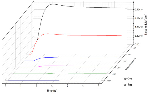
(a) The temporal distribution of total electric field at different heights on XoY cross section. (b) The trend of electric field strength, when x = 0 m, y = 15 m and z = 1 m.

Based on the research on the total electric field in the horizontal direction, this section mainly concentrates on the dynamic distribution and variation law of electric field at comparatively close distance.

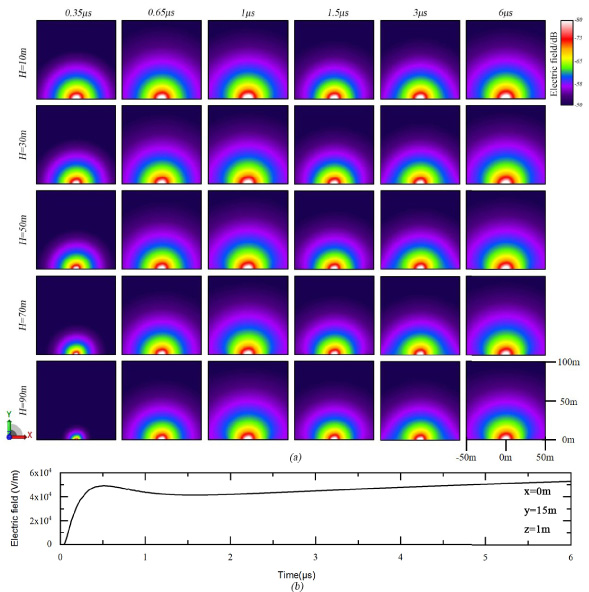
The dynamic distribution of total electric field at different heights is depicted in Fig. 4(a). On the whole, the distribution of total electric field looks like a cylinder. Aiming at observing the variation of distribution expediently, the unit of decibel and the benchmark of 6 ×10⁷ V/m are adopted to manifest the distinction of different field strengths. With the same time, the electric field distribution zone gradually reduces as the height increases, and its field strength gradually diminishes along the positive direction of y-axis. This spatial evolution is in relation to fact that the return stroke current propagates along the longitudinal channel, chiefly radiating electrostatic field at close distance. Moreover, with the identical height, the total electric field increases at first then decreases and increases again. Although there are changes in electric field distribution from 0.65 μs to 6 μs at the same height, the changes are little. The trend of outer edge of the electric field distribution conforms to the electric waveform shown in Fig. 4(b), which emanates the changes of the total electric field located in the position away from the return point 15 m and at the height of 1 m. And the temporal variation trend of Fig. 4(b) is consistent with that of Fig. 3. In addition, the variation of total electric field as heights increase depicted in Fig. 4(a) is in good agreement with the variation trend of electric field strength peak shown in Fig. 5.

Fig. 5.

The field strength peaks of E _z component and total electric field at different heights, when x = 0 m and y = 30 m.

The electric field strength peak of both E _z component and total electric field in the region near the source decreases with height, which is shown in Fig. 5. And the decay rate of the peak of total electric field is smaller than that of E _z component on account of the first derivative of electric field strength peaks. And the peaks of E _z at different heights account for 92.69%, 87.79%, 74.56%, 60.24%, 48.15%, 38.65%, 29.37%, 26.07%, 20.72%, 16.55% and 14.80% respectively of the total electric field strength peaks, which demonstrates that the proportion of the E _z component in the total electric field of the LEMP decreases with height. The field strength of vertical component of lightning return stroke electric field in the region near the ground is much larger than that of the horizontal component at the same position [43,44], which is consistent with the phenomenon in Fig. 5. Considering the distribution of total electric field at different heights depicted in Fig. 4 and the peaks of total electric field at different heights shown in Fig. 5, it can be found that electric field attenuates slightly as height increases after the initial peak of the electric field.

In accordance to Fig. 6, the distribution of E _z component at close distance looks like the sphere, whose radius increase with time. The distribution shape of E _z component in above figure associates the distribution phenomenon of electric field component under the ground in literature [45], and both the distributions of electric field E _z components in the aerial and underground region take on spherical distribution. The distribution structure of E _z component resembles cylinder, which is different from the distribution of E _x and E _y. And the distribution of E _x and E _y has been discussed in our another paper [46]. In addition, the peak of field strength of E _z component gradually declines with height rising. The reason for the attenuation phenomenon of E _z along radial direction is that electrostatic field, which is the dominant field component in the region close to the channel-base current source, is inversely proportional to distance r ³ according to the formula (2) [47].

Fig. 6.

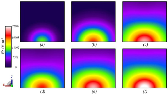
The electric field transient distribution of E _z component on XoZ cross section when X = −50 ∼ 50 m, Y = 30 m, Z = 0 ∼100 m. (a) 0.2 μs. (b) 0.3 μs. (c) 0.6 μs. (d) 2 μs. (e) 5 μs. (f) 8 μs.

3.1.2. Magnetic field

Considering the simulation results of total magnetic field within the horizontal range of 0 ∼ 1000 m, at the height of 6 m depicted in the Fig. 7, the magnetic field strength, at first, rapidly soars, and then gradually diminishes. The temporal variation features of the magnetic field at different distances are consistent with the measured magnetic field result [35]. What’s more, as horizontal distance increases, that magnetic field strength also rapidly attenuates, which is confirmed by the equation (3), verifies induction field, whose field strength highly depends on the distance between field point and the source point, dominates the return stroke magnetic field at close distance.

Fig. 7.

Magnetic field strengths with distance to the channel is 15 m, 30 m, 150 m, 300 m, 600 m and 900 m, when x = 0 m and z = 6 m.

To further investigate the magnetic field at close distance, then this section further discuss the evolution process and the distribution traits of the magnetic field along the vertical direction, which is comparatively closer to the channel.

The evolution of total magnetic field distribution at different heights is shown in Fig. 8(a). Likewise, 8 ×10⁴ A/m is adopted as the benchmark for the unit of decibel. The total magnetic field distribution zone gradually shrinks at time of 0.32 μs as height rises, and its variation of field strength along y-axis is akin to that of electric field. When at other times (after 0.65 μs), the distribution zone changes slightly at the same time as height increases. Furthermore, the total magnetic field strength increases at first then descends at the same height over time, and conspicuously the magnetic field distribution zone at 0.65 μs is larger than those at any other time, which is stimulated by the peak of return stroke current. And the magnetic field distribution zone obviously attenuates as time augments after the initial peak of the magnetic field. The variation of temporal distribution zone at same height is consistent with the temporal variation trend of magnetic field shown in Fig. 8(b), which is similar to that of magnetic field depicted in the Fig. 7.

Fig. 8.

(a) The temporal distribution of total magnetic field at different heights on XoY cross section. (b) The trend of magnetic field strength, when x = 0 m, y = 15 m and z = 1 m.

In Fig. 9, the peaks of field strength of total magnetic field and H _x component have the relatively similar decay rate. And the peaks of H _x at different heights account for average of 97.91% of the total magnetic field, which illustrates that H _x component dominates the distribution of magnetic field in the region. Additionally, magnetic field can be divided into high and low frequency magnetic field. It is generally assumed that the frequency of the low-frequency magnetic field is below 100 kHz [48]. The frequency domain of lightning is assumed to be in the range of direct current (DC) to 5 MHz [49]. According to Fig. 10, the majority of magnetic field amplitude at close distance mainly concentrate on frequency of the low-frequency.

Fig. 9.

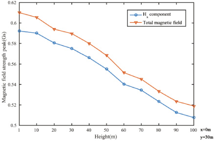
The field strength peaks of H _x component and total magnetic field at different heights, when x = 0 m and y = 30 m.

Fig. 10.

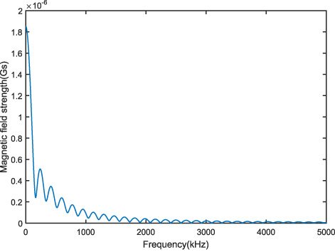
The frequency spectrum of the magnetic field, when x = 0 m, y = 30 m and z = 1 m.

The distribution of H _x, the dominant field component in the region, is shown in Fig. 11. The distribution of H _x component, which resembles multi-layer columnar structure, is similar to that of H _y, which has been researched in our another paper [46]. The distribution phenomenon is attributed to the Ampere Rule [50]. Besides, the magnetic field stimulated by the return stroke current along the channel presents symmetrical distribution. At the beginning of the process, field strength gradually magnify until the maximum value produced by the peak of channel current appears. Moreover, the distance-varying law of field strength of H _x component can be regarded as an analogy of the distribution of E _z component. The distance from the observation point to the return stroke point larger is, and the magnetic field strength smaller is. This distribution phenomenon is complied with relation between the field strength and distance from the formula (3) [31].

Fig. 11.

The magnetic field transient distribution of H _x component on XoZ cross section when X = −50 ∼ 50 m, Y = 30 m, Z = 0 ∼100 m. (a) 0.2 μs. (b) 0.3 μs. (c) 0.6 μs. (d) 1.1 μs. (e) 3 μs. (f) 6 μs.

3.2. The distribution of Poynting vector at close distance

According to the simulation results of total Poynting vector within the horizontal range of 0 ∼ 1000 m, at the height of 6 m depicted in the Fig. 12, the variation tendency of waveform of Poynting vector is similar to the features of total magnetic field depicted in Fig. 7. Moreover, compared with the field strength trend of electric field and magnetic field, the peak of total Poynting vector diminishes more rapidly as horizontal distance increases. According to equation (4), which reveals the quantity relation between electric field, magnetic field and Poynting vector, that total Poynting vector diminishes more rapidly as horizontal distance increases can be deduced on the basis of the attenuation trends depicted in Fig. 3 and 7.

Fig. 12.

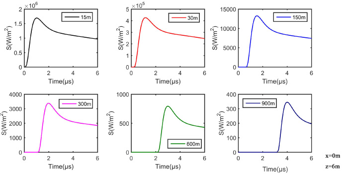
The Poynting vector with distance to the channel is 15 m, 30 m, 150 m, 300 m, 600 m and 900 m, when x = 0 m andz = 6 m.

On basis of the research on the total Poynting vector in the horizontal direction, this section mainly discusses the dynamic distribution and variation features of Poynting vector at different height in the region much closer to the lightning channel.

The Poynting vector of electromagnetic field stimulated by CG flashes denotes the electromagnetic energy. Except for the field strength, the Poynting vector also can be used to signify the energy characteristics of LEMP so that the distribution and hazard of LEMP can be analyzed comprehensively by the synthetical analysis of electromagnetic field. The temporal distribution of Poynting vector at different heights is depicted in Fig. 13(a). Similarly, 4 ×10¹² W/m² is adopted as the benchmark for the unit of decibel. With the same time, the Poynting vector distribution zone gradually reduces as the height increases. According to Fig. 13, the distribution of total Poynting vector increases at first then decreases at same height over time, and its variation trend is similar to the waveform of Poynting vector shown in Fig. 13(b). Meanwhile, the variation trends of the Poynting vector waveform depicted in Fig. 13(b) and Fig. 12 are uniform.

Fig. 13.

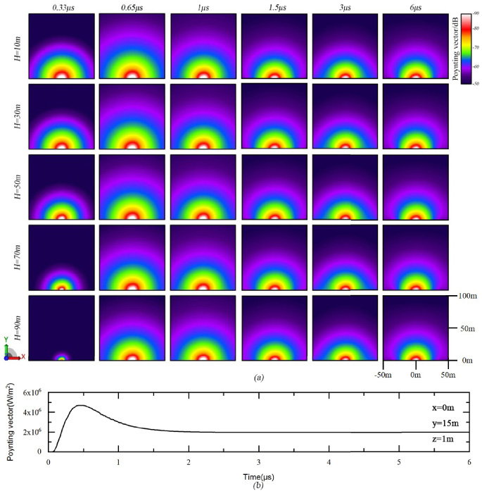
(a) The temporal distribution of total Poynting vector field at different heights on XoY cross section. (b) The trend of Poynting vector, when x = 0 m, y = 15 m and z = 1 m.

The variation with height of the total Poynting vector and its different components in the Cartesian coordinates is displayed in Fig. 14. The variation trend of S _x and S _y component is similar to that of the total Poynting vector, but the decay rate of two components is larger than that of total Poynting vector. In addition, it’s obvious that the order of magnitude of S _x component is smaller than others for the reason that S _x is calculated by cross product of electric field, in which the horizontal components of electric field significantly smaller than the vertical component [43,44], and magnetic field with minor unit. Furthermore, the magnitude of S _z component conspicuously increases at the early time, and then slowly declines later.

Fig. 14.

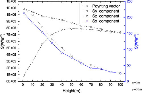
The peaks of electromagnetic energy of total Poynting vector and its components at different heights, when x = 0 m and y = 30 m. The value of total Poynting vector, S _y component and S _z component associates with the left y-axis. The value of S _x component associates with the right y-axis.

The dynamic distribution of S _x component on YoZ cross section is shown in Fig. 15. The distribution shape of S _x component seems like a streamlined cylinder. As the return stroke current propagates along the channel, electromagnetic energy continuously diffuses along z-axis positive direction. When the peak of S _x component emerges, the electromagnetic energy sets about attenuating. Simultaneously, the energy constantly radiates with the increment of time, and attenuates along the positive direction of y-axis.

Fig. 15.

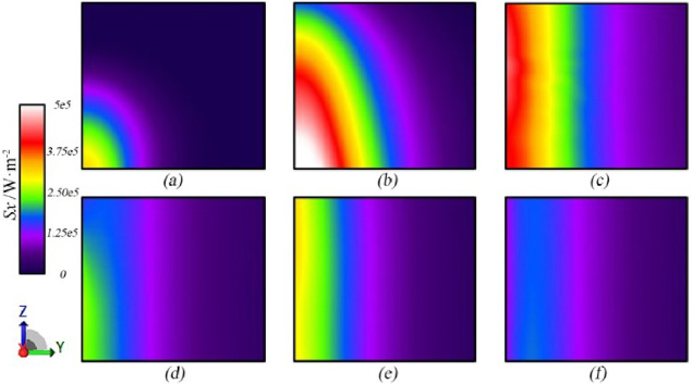
The transient distribution of S _x component of Poynting vector on YoZ cross section when X = 40 m, Y = 0 ∼100 m,Z = 0 ∼100 m. (a) 0.3 μs. (b) 0.5 μs. (c) 1 μs. (d) 2 μs. (e) 4 μs. (f) 6 μs.

In general, the distribution of S _y component resembles spheroidicity. Compared with S _x component, the magnitude of S _y component does not continuously diffuse along the z-axis. The major electromagnetic energy distributes in the region near the ground. The magnitude of S _y component gradually descends along the radial direction with time increasing. The height-varying attenuation of S _y component in Fig. 16 is in accord with the variation of the peak of S _y component at different heights shown in Fig. 14.

Fig. 16.

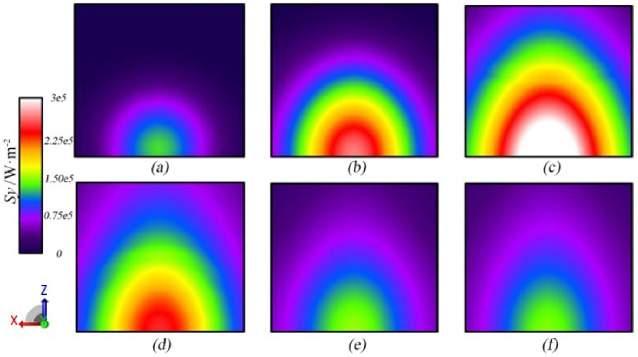
The transient distribution of S _y component of Poynting vector on XoZ cross section when X = −50 ∼50 m, Y = 50 m,Z = 0 ∼100 m. (a) 0.3 μs. (b) 0.4 μs. (c) 0.6 μs. (d) 1 μs. (e) 4 μs. (f) 8 μs.

The transient distribution of S _z component in the process of lightning return stroke is depicted in Fig. 17. According to the peak distribution of S _z in Fig. 14, the fact that S _z evolves as the dominant component in the region near the source indicates that the order of magnitude of S _z is a considerable quantity so that the unit of decibel with the benchmark of 1.7 ×10¹² W/m² is adopted to describe the dynamic process of S _z component. The distribution shape of S _z component is similar to that of E _z component, which takes on sphericity. Whereas the electromagnetic energy of S _z component continually diffuses along the radial direction. There are no obvious changes in the latter part of Fig. 17, which is analogous with the waveform trend of Poynting vector peak of S _z.

Fig. 17.

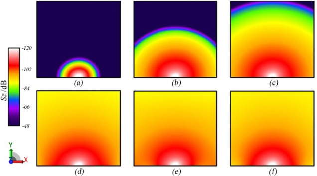
The transient distribution of S _z component of Poynting vector on XoY cross section when X = −50 ∼ 50 m, Y = 0 ∼100 m, Z = 60 m. (a) 0.2 μs. (b) 0.3 μs. (c) 0.4 μs. (d) 2 μs. (e) 5 μs. (f) 8 μs.

4. Conclusion

In this paper, the distribution of lightning return stroke electromagnetic field close to the channel-base source is analyzed to clarify the field strength and electromagnetic energy of LEMP based on the numerical simulation of 3D model of lightning return stroke in XFDTD software. On the basis of above simulation results, we draw the following conclusions.

(1) The distribution of total electric field in the region resembles the cylinder, and that of E _z component resembles the sphere. However, the distribution structure of E _z, which is akin to cylinder is different from that of E _x and E _y. The distribution area of total electric field decreases as height increases, and enlarges firstly then diminishes, enlarges again as time increase. Moreover, the electric field waveform depicted in Fig. 4(b) will approximately keep the strength of about 5 ×10⁴ V/m after the waveform reaching the peak electric field. Hence, the hazard from the electric field might be continuous during the process of return stroke. Meanwhile the E _z is the dominant component near the ground, and its peak of field strength declines with the increment of height. Therefore, it is noted that the research about distribution of E _z component conduces to the improving of the protection of induced overvoltage to the electronic devices.

(2) The distribution area of total magnetic field decreases as height increases, and expands firstly then shrinks as time increase. And the H _x component, whose distribution looks like columnar structure, always dominates the peak of the total magnetic field. The distribution of H _y component is akin to that of H _x. Furthermore, the dynamic distribution of magnetic field closely associates with the variation of waveform of channel-base current. Hence, that the magnetic field waveform shown in Fig. 8(b) will promptly decline after emergence of the magnetic field peak value reveals that the correlation between magnetic field waveform and the current, but also the hazard of the magnetic field with the feature of fleeting single pulse may also have impact on the adjacent devices during the return stoke. Accordingly, the magnetic field characterized by low frequency is a kind of electromagnetic interference source, which is difficult for electronic equipments to circumvent the magnetic hazard.

(3) The dynamic process of Poynting vector denotes the distribution of electromagnetic energy stimulated by the return stroke current. In terms of qualitative analysis, the distribution of each component takes on symmetrical structure. The spatial and temporal evolution of distribution of total Poynting vector is similar to that of total magnetic field. Meanwhile the S _x component of Poynting vector resembles streamlined cylinder, and S _y spheroidicity, and S _z sphere. According to quantitative analysis, total Poynting vector of LEMP gradually attenuates as the height increases.The S _x and S _y component are characterized by the similar trend. Then, S _z emerges as the dominant component in the region as height augments, which should warrant the due attention to the electromagnetic hazard from the S _z component. Furthermore, the total Poynting vector waveform that changes over time also embodies the fleeting single pulse depicted in Fig. 13(b), which may elucidate the hazard of electromagnetic energy instantaneously transforms. Meanwhile, that the order of magnitude of Poynting vector of LEMP at close distance suggests that electromagnetic energy from the LEMP might pose a potential threat to electronic equipments.

(4) Furthermore, it’s worth noting that the trend of field strength and electromagnetic energy changes with height at close distance. The trends of components of electromagnetic field and energy are different, albeit the amplitudes of total electric field, total magnetic field and total Poynting vector descends with height increases. Except for S _z component shown in Fig. 14, the peaks of other components mentioned above diminish as heights increases. The impacts of components are also worthy of our attention. The problem about electromagnetic hazard should be considered by total field strength at some fixed-positions, but also the hazard from predominant components at different heights to the devices adjacent to the return stroke point. Therefore, the protection of LEMP should be based on the comprehensive analysis of field strength and electromagnetic energy.

Footnotes

Acknowledgements

This work is supported in part by the National Natural Science Foundation of China (No. 41375012) and the Beijing Natural Science Foundation Program (No. KZ201411232037).

References

Rakov

V.A.

, Fundamentals of Lightning, Cambridge University Press, Cambs, 2016.

Rakov

V.A.

and Rachidi

, Overview of recent progress in lightning research and lightning protection, IEEE Transactions on Electromagnetic Compatibility 51(3) (2009), 428–442, doi:10.1109/TEMC.2009.2019267.

Uman

M.A.

and McLain

D.K.

, Magnetic field of lightning return stroke, Journal of Geophysical Research 74(28) (1969), 6899–6910, doi:10.1029/jc074i028p06899.

Rakov

V.A.

, Calculated electromagnetic fields of lightning return stroke, Tekh. Elektrodinam. 1 (1987), 87–89.

Nucci

C.A.

, On lightning return stroke models for LEMP calculations, in: Proc. 19th Int. Conf. Lightning Protection, Graz, Austria, 1988.

Bruce

C.E.R.

and Golde

R.H.

, The lightning discharge, Journal of the Institution of Electrical Engineers-Part II: Power Engineering 88(6) (1941), 487–505, doi:10.1049/ji-2.1941.0065.

Heidler

, Traveling current source model for LEMP calculation, in: Proc. 6th Int. Zurich Symp. Electromagnetic Compatibility, Zurich, Switzerland, 1985.

Heidler

Cvetic

J.M.

and Stanic

B.V.

, Calculation of lightning current parameters, IEEE Transactions on Power Delivery 14(2) (1999), 399–404, doi:10.1109/61.754080.

Yazhou

Shanghe

Xiaorong

A new kind of lightning channel-base current function, in: 3rd International Symposium on Electromagnetic Compatibility, Beijing, China, 2002.

10.

Harrington

R.F.

, Field Computation by Moment Methods, Wiley-IEEE Press, 1993.

11.

Yee

, Numerical solution of initial boundary value problems involving Maxwell’s equations in isotropic media, IEEE Transactions on Antennas and Propagation 14(3) (1966), 302–307, doi:10.1109/TAP.1966.1138693.

12.

Sadiku

M.N.O.

, A simple introduction to finite element analysis of electromagnetic problems, IEEE Transactions on Education 32(2) (1989), 85–93, doi:10.1109/13.28037.

13.

Ruehli

A.E.

, Equivalent circuit models for three-dimensional multiconductor systems, IEEE Transactions on Microwave Theory and Techniques 22(3) (1974), 216–221, doi:10.1109/tmtt.1974.1128204.

14.

Haddad

M.A.

Rakov

V.A.

and Cummer

S.A.

, New measurements of lightning electric fields in Florida: Waveform characteristics, interaction with the ionosphere, and peak current estimates, Journal of Geophysical Research: Atmospheres 117(D10) (2012), doi:10.1029/2011JD017196.

15.

and Cummer

S.A.

, An FDTD model for low and high altitude lightning-generated EM fields, IEEE Transactions on Antennas and Propagation 54(5) (2006), 1513–1522, doi:10.1109/TAP.2006.874336.

16.

Shoory

Mimouni

Rachidi

, Validity of simplified approaches for the evaluation of lightning electromagnetic fields above a horizontally stratified ground, IEEE Transactions on Electromagnetic Compatibility 52(3) (2010), 657–663, doi:10.1109/temc.2010.2045229.

17.

Zhang

Wang

, Computation of lightning horizontal field over the two-dimensional rough ground by using the three-dimensional FDTD, IEEE Transactions on Electromagnetic Compatibility 56(1) (2013), 143–148, doi:10.1109/temc.2013.2266479.

18.

Yang

and Zhou

, Calculation methods of electromagnetic fields very close to lightning, IEEE Transactions on Electromagnetic Compatibility 46(1) (2004), 133–141, doi:10.1109/temc.2004.823626.

19.

Baba

and Rakov

V.A.

, Influence of strike object grounding on close lightning electric fields, Journal of Geophysical Research: Atmospheres 113(D12) (2008), doi:10.1029/2008JD009811.

20.

Zhang

Liu

, Validation of the Cooray-Rubinstein (C-R) formula for a rough ground surface by using three-dimensional (3-D) FDTD, Journal of Geophysical Research: Atmospheres 118(22) (2013), 12749–12754, doi:10.1002/2013JD020078.

21.

Khosravi-Farsani

Moini

Sadeghi

S.H.H.

, On the validity of approximate formulas for the evaluation of the lightning electromagnetic fields in the presence of a lossy ground, IEEE Transactions on Electromagnetic Compatibility 55(2) (2012), 362–370, doi:10.1109/TEMC.2012.2211364.

22.

Mimouni

Rachidi

and Rubinstein

, Electromagnetic fields of a lightning return stroke in presence of a stratified ground, IEEE Transactions on Electromagnetic Compatibility 56(2) (2013), 413–418, doi:10.1109/TEMC.2013.2282995.

23.

Zhang

Fan

, Examination of the Cooray-Rubinstein (C-R) formula for a mixed propagation path by using FDTD, Journal of Geophysical Research: Atmospheres 117(D15) (2012), doi:10.1029/2011JD017331.

24.

Sobrinho

C.L.S.S.

, Computational environment for simulating lightning strokes in a power substation by finite-difference time-domain method, IEEE Transactions on Electromagnetic Compatibility 51(4) (2009), 995–1000, doi:10.1109/temc.2009.2028879.

25.

Omari

and Mimouni

, Electromagnetic fields at very close range from a tower struck by lightning in presence of a horizontally stratified ground, IEEE Transactions on Electromagnetic Compatibility 61(1) (2018), 166–173, doi:10.1109/TEMC.2018.2790166.

26.

Soto

Perez

and Herrera

, Electromagnetic field due to lightning striking on top of a cone-shaped mountain using the FDTD, IEEE Trans. Electromagn. Compat. 56(5) (2014), 1112–1120.

27.

Khosravi

Sadeghi

S.H.H.

and Moini

, Electromagnetic field due to lightning strike to a tall tower sitting on a mountainous terrain, IEEE Transactions on Electromagnetic Compatibility 58(4) (2016), 1–10.

28.

Zhang

and Wu

, A new perspective to the attributes of lightning electromagnetic field above the ground, Journal of Electrostatics 71(4) (2013), 703–711, doi:10.1016/j.elstat.2013.03.014.

29.

Uman

M.A.

Mclain

D.K.

and Krider

E.P.

, The electromagnetic radiation from a finite antenna, American Journal of Physics 43(1) (1975), 33–38.

30.

Nucci

C.A.

Diendorfer

Uman

M.A.

, Lightning return stroke current models with specified channel-base current: A review and comparison, Journal of Geophysical Research: Atmospheres 95(D12) (1990), 20395–20408, doi:10.1029/jd095id12p20395.

31.

Ren

Tian

, Examining the influence of current waveform on the lightning electromagnetic field at the altitude of halo formation, Journal of Atmospheric and Solar-Terrestrial Physics 189 (2019), 114–122, doi:10.1016/j.jastp.2019.04.010.

32.

M’ziou

Mokhnache

Boubakeur

, Validation of the Simpson-finite-difference time domain method for evaluating the electromagnetic field in the vicinity of the lightning channel initiated at ground level, IET Generation, Transmission & Distribution 3(3) (2009), 279–285, doi:10.1049/iet-gtd:20080342.

33.

Rakov

V.A.

and Uman

M.A.

, Review and evaluation of lightning return stroke models including some aspects of their application, IEEE Transactions on Electromagnetic Compatibility 40(4) (1998), 403–426, doi:10.1109/15.736202.

34.

Baba

and Rakov

V.A.

, On the transmission line model for lightning return stroke representation, Geophysical Research Letters 30(24) (2003), doi:10.1029/2003gl018407.

35.

Uman

M.A.

Schoene

Rakov

V.A.

, Correlated time derivatives of current, electric field intensity, and magnetic flux density for triggered lightning at 15 m, Journal of Geophysical Research: Atmospheres 107(D13) (2002), ACL 1-1–ACL 1-11, doi:10.1029/2000JD000249.

36.

Uman

M.A.

Rakov

V.A.

Rambo

K.J.

, Triggered-lightning experiments at Camp Blanding, Florida (1993–1995), IEEJ Transactions on Power and Energy 117(4) (1997), 446–452, doi:10.4271/1999-01-2413.

37.

Rakov

V.A.

, Some inferences on the propagation mechanisms of dart leaders and return strokes, Journal of Geophysical Research: Atmospheres 103(D2) (1998), 1879–1887, doi:10.1029/97jd03116.

38.

Moini

Nazari

Fortin

, On the use of the antenna theory model of lightning return stroke with distributed current source for EMC analysis, IEEE Transactions on Electromagnetic Compatibility 61(3) (2019), 674–680, doi:10.1109/TEMC.2019.2897084.

39.

Moini

Kordi

Rafi

G.Z.

, A new lightning return stroke model based on antenna theory, Journal of Geophysical Research: Atmospheres 105(D24) (2000), 29693–29702, doi:10.1029/2000jd900541.

40.

Chorlton

L.B.

, Generalized geology of the world: bedrock domains and major faults in GIS format: A small-scale world geology map with an extended geological attribute database, Geological Survey of Canada, Open File 5529, doi:10.4095/223767.

41.

Horton

J.D.

San Juan

C.A.

and Stoeser

D.B.

, The State Geologic Map Compilation (SGMC) geodatabase of the conterminous United States, U.S. Geological Survey Data Series 1052, doi:10.3133/ds1052.

42.

Tatematsu

Rachidi

and Rubinstein

, Analysis of electromagnetic fields inside a reinforced concrete building with layered reinforcing bar due to direct and indirect lightning strikes using the FDTD method, IEEE Transactions on Electromagnetic Compatibility 57(3) (2015), 405–417, doi:10.1109/temc.2015.2400132.

43.

Yang

Qie

X.S.

Wang

J.G.

, Observation of the lightning-induced voltage in the horizontal conductor and its simulation, Acta Physica Sinica 3 (2008), 1968–1975, doi:10.1016/j.tsf.2007.04.123.

44.

Miki

Rakov

V.A.

Rambo

K.J.

, Electric fields near triggered lightning channels measured with Pockels sensors, Journal of Geophysical Research: Atmospheres 107(D16) (2002), ACL 2-1–ACL 2-11, doi:10.1029/2001jd001087.

45.

Zhang

, Distribution characteristics of lightning electromagnetic pulsed fields under the ground, Acta Physica Sinica 62(2) (2013), 709–712, doi:10.7498/aps.62.029202.

46.

Zhang

Tian

Wang

Research on the distribution characteristics of electromagnetic environment in the lightning return stroke near-field area, in: 2019 International Symposium on Antennas and Propagation (ISAP), Xi’an, China, 2019.

47.

Wang

Sun

Tian

, Current full-waveform inversion of the return stroke channel based on single-station electric field observations, Radio Science 53(10) (2018), 1245–1253, doi:10.1029/2018RS006557.

48.

Gajsek

Ravazzani

Grellier

, Review of studies concerning electromagnetic field (EMF) exposure assessment in Europe: Low frequency fields (50 Hz–100 kHz), International Journal of Environmental Research and Public Health 13(9) (2016), 875, doi:10.3390/ijerph13090875.

49.

Akbari

Sheshyekani

Pirayesh

, Evaluation of lightning electromagnetic fields and their induced voltages on overhead lines considering the frequency dependence of soil electrical parameters, IEEE Transactions on Electromagnetic Compatibility 55(6) (2013), 1210–1219, doi:10.1109/TEMC.2013.2258674.

50.

Yang

Qie

Zhang

, Magnetic field measuring system and current retrieval in artificially triggering lightning experiment, Radio Science 43(2) (2008), doi:10.1029/2007RS003753.

Lightning return stroke electromagnetic field and energy at close distance by using 3D FDTD simulation

Abstract

Keywords

1. Introduction

2. Method and computational models

2.1. The lightning electromagnetic field method

2.2.2. The excitation source of the model

Table 1 Parameters of fitting current waveform I 1/ (kA) I 2/ (kA) τ1∕μs τ2∕μs τ3∕μs τ4∕μs 6.55 4.00 9.00 0.22 90.90 100.00

3. Simulation results and discussion

3.1. The lightning return stroke electromagnetic field at close distance

3.1.1. Electric field

Footnotes

Acknowledgements

References

Table 1
Parameters of fitting current waveform

I ₁/ (kA) I ₂/ (kA) τ₁∕μs τ₂∕μs τ₃∕μs τ₄∕μs

6.55 4.00 9.00 0.22 90.90 100.00