Virtual Halbach analytical method for improved Halbach magnetized PM slotless planar linear actuators

Abstract

This paper proposes a new virtual Halbach analytical method for improved Halbach permanent magnet (PM) slotless planar linear actuators, which have mixed neodymium iron baron (NdFeB) magnets and ferrite magnets to form a two-segment quasi-Halbach topology with different heights of main and auxiliary magnetic poles. The method has four steps, which are described in detail in the paper. One of the key steps is to visually regard the permanent magnet region magnetized only in the y direction as a Halbach array structure with a magnetization amplitude of 0 in the x direction that satisfies the Newman boundary condition. The investigation shows that the results of the new analytical method are in good agreement with the finite element method. Using this analytical method, the effect of improved Halbach permanent magnet slotless planar linear actuator with unequal height of the main and auxiliary magnetic poles on the magnetic field waveform is analyzed by means of a parametric research.

Keywords

Analytical Halbach magnetic field permanent magnet (PM)

1. Introduction

Since the high-performance NdFeB were developed in early 1980's, permanent magnet actuators using NdFeB have been able to provide high power density and high efficiency [1], and are becoming increasingly popular in industrial field and domestic appliances, especially electric vehicles, wind power and wave power generation, etc. However, due to the rapid increase in the price of NdFeB in recent years, the awareness of saving the cost of permanent magnets while pursuing the improvement of the air-gap magnetic performance of the actuator is increasing [2]. Exploring new technologies, such as Halbach magnetization structure [3–7], magnet segmentation [8–15], magnet-shaping technique [16–20], and stepped magnet pole [21–24], creating magnet pole with different magnet materials [25,26], etc., are all improving performance and reducing cost awareness. Although the new technologies mentioned above have strong advantages from a certain point of view, but there are many disadvantages, so there are literatures [2–4,10] that combine two or more of them to achieve better performance. Among them, Halbach topology technology [6], especially the Halbach topology combined with other technologies, has outstanding self-shielding properties, and has been sought after by scholars. Firstly, the following summarizes several typical improved Halbach structures. For the improved Halbach structure, scholars [2–4,10,23,27,29–31] have obtained some valuable research results from different structural, magnetization directions, permanent magnet materials and so on. In particular, some scholars considered more Halbach parameters. For example, combining the merits of Halbach magnetization with two magnetic materials and modular pole technique, Shen et al. [2] achieved better performance in machine, but instead of giving an analytical method, the more complicated subdomain analytical method [28] is used. However, for their proposed complex Halbach structure, Shen et al. did not analyze and discuss the influence of the residual magnetization of permanent magnet materials on the magnetic field. Secondly, for the Halbach structure and the improved Halbach structure, the methods are usually analytical methods, 3D modeling, finite element method, subdomain model method [24,28,29,32–35], etc., but the improved Halbach structure is more complicated and difficult to obtain analytical methods. Then, considering the Halbach structure combined with other technologies that comprehensively meets the requirements of reducing structural complexity, reducing costs, and improving performance, it is very difficult to obtain analytical solutions, usually replaced by a finite element method. Therefore, the Halbach structure with two-stage main and auxiliary magnetic pole heights selected in this paper is a better compromise to meet these conditions. Due to the Halbach structure with different heights of main and auxiliary magnetic poles, the extra non-magnetized regions cause an increase in permanent magnet partitioning, making it difficult to adopt a general analytical method. Finally, in response to this problem, this paper proposes a new analytical method, which is different from the subdomain model and other methods mentioned above.

In this paper, a new virtual Halbach analytical method is proposed for the Halbach permanent magnet slotless planar linear actuator with different heights of main and auxiliary magnetic poles. In Section 2, the analytic method is validated by finite element method. In Section 3, this analytic method is used to optimize the Halbach topology using parameters closely related to the shape of the magnetic pole and the magnetic flux density. Section 4 discusses the effects of three parameters on the air gap magnetic field, namely the ratio of the auxiliary magnetic pole to main magnetic pole in the magnetization direction, the ratio of the auxiliary magnetic pole to the pole pitch in the x direction, and remanence density of the auxiliary magnetic pole.

This paper contributions are (1) the new virtual Halbach analytical method is proposed to solve the magnetic field with two-segment Halbach array of different heights of main and auxiliary magnetic poles, and is validated by finite element method, and (2) the parametric research with the method, whose parameters are closely related to the shape of the magnetic pole and the magnetic flux density, are used to optimize the improved Halbach magnetized permanent magnet topology.

2. Analytical model

2.1. Model description and assumptions

Figure 1 shows a slotless permanent magnet planar linear actuator in which the permanent magnets are in an improved Halbach array topology. The traditional quasi-Halbach array structure is formed by splicing two or more regular square permanent magnets, and the magnetic pole height of the main and auxiliary magnetizing magnets is equal, as shown in Fig. 2(a). By changing the shape of the conventional magnetic pole, there is better performance in the actuator magnetic field, namely magnet-shaping technology. Figure 2(b) shows a relatively simple unequal height magnet-shaping magnetic pole based on the conventional two-segment quasi-Halbach array structure. This paper will describe the analytical means to enhance the airgap magnetic field in planar linear actuator by varying the magnetizing magnet height in x and y directions, and by changing the magnetizing magnet widths of the main and auxiliary poles, namely Ly and Lx, and by replacing the remanence magnetic material with different remanence in the x direction, namely B _rx.

Fig. 1.

Schematic diagram of slotless permanent magnet planar linear actuator.

Fig. 2.

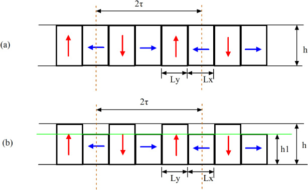
Quasi-Halbach magnetization pattern. (a) Regular square permanent magnets. (b) Unequal height permanent magnets in the two magnetization directions of x and y.

In order to obtain the solution of the analytical equation of the model of Fig. 2(b), planar linear actuator is divided in several regions as shown in Fig. 3. In this model, the following assumptions are made:

(1) the soft magnetic core portion is infinite magnetic permeability and unsaturated;

(2) the actuator is sufficiently long, so end-effects are ignored;

(3) the back iron is unsaturated and eddy current and hysteresis loss in it are all neglected;

(4) all magnets operate on a linear demagnetization curve, and have been fully magnetized in the magnetization direction.

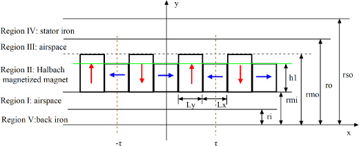
2.2. Proposal of the virtual Halbach analytical method

In order to better analyze this model, a high-low coercivity hybrid Halbach permanent magnet linear actuator analysis model is established as shown in Fig. 3. The two arrow colors represent two different material permanent magnets, that is, red indicates high coercive permanent magnet material, and blue indicates a low-coercive permanent magnet material, respectively. The arrow direction in Fig. 3 indicates the magnetization direction of the permanent magnet, that is, the red arrow indicates the high-coercive permanent magnet magnetization direction, and the blue arrow indicates the low-coercive permanent magnet magnetization direction. The layered processing of the quasi-Halbach structure topology actuator model of Fig. 2(b) can divide the five-layer model as shown in Fig. 3, namely, airspace region I, PM region II, the air-gap region III, stator iron region IV, and back iron region V. The boundary conditions where y = ro, y = rmi and y = ri, are all corresponding to the Neumann boundary conditions.

Due to the different heights of the high and low coercive permanent magnets, a green layered line as shown for the region II in Fig. 3 is proposed, and then the region II is subdivided into two regions, which are defined as region II1 and region II2, i.e., II1 is the lower part of the permanent magnet region, and II2 is the upper part. As shown in Fig. 4, after dividing the region II into two regions II2 and II1, region II1 is a quasi-Halbach topology, and region II2 can be regarded as a quasi-Halbach topology in which the residual magnetization vector Mx in the x direction is 0, that is, the x-direction permanent magnets are not magnetized in the region II2. Therefore, the upper boundary of region II and II2 is y = rmo, which satisfies the Newman boundary condition, and the lower boundary of region II and II1 is y = rmi, which also satisfies the Newman boundary condition. The upper boundary of region II1 coincides with the lower boundary of II2, i.e., y = rmi + h1, and meets Neumann boundary conditions. In calculating the magnetic density of the region II to the air gap, the quasi-Halbach boundary conditions are used to calculate the flux density of the region II1 and II2 to the air gap, respectively. Then, using the superposition principle, the air gap flux density of region II can be calculated. That is to say, firstly, when calculating the magnetic flux density of the air gap of the region II1, the air is filled with the region II2 to solve the equation; Secondly, when calculating the magnetic flux density of the air gap of II2, air filling is performed on the region II1, and the residual magnetization in the x direction of the II2 region is set to 0, and the solution of the equation can be obtained; Finally, the magnetic flux density obtained by the previous two steps is superimposed to obtain the flux density of the region II to the air gap.

Since, in the calculation of the magnetic field of the region II2, the region II2 adopts the boundary condition of the Halbach array while adding two other conditions, namely, setting the residual magnetization parameter Mx = 0 in the x direction and unchanging the residual magnetization parameter My value in the y direction. That is to say, the region II2 is regarded as a virtual satisfying Halbach boundary condition, and then the magnetic fields of II1 and II2 are respectively calculated, and finally the magnetic flux density of the region II to the air gap is calculated by applying the magnetic field superposition principle. Therefore, this analysis method is called virtual Halbach analytical method in this paper.

Fig. 3.

Quasi-Halbach structure region model.

Fig. 4.

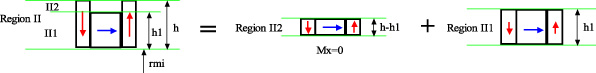
Flux density equivalent calculation model of region II with virtual Halbach analytical method.

2.3. Governing equations

For linear PM actuators, the flux density vector and magnet field intensity vector in regions I, II and III, are respectively coupled by $\begin{eqnarray}\displaystyle \text{} & \text{} & \displaystyle \vec{B}_{I}={\mu}_{0}{\mu}_{rI}\vec{H}_{I}\end{eqnarray}$ (1) $\begin{eqnarray}\displaystyle \text{} & \text{} & \displaystyle \vec{B}_{II}={\mu}_{0}{\mu}_{rII}\vec{H}_{II}+{\mu}_{0}\vec{M}_{0}\end{eqnarray}$ (2) $\begin{eqnarray}\displaystyle \text{} & \text{} & \displaystyle \vec{B}_{III}={\mu}_{0}{\mu}_{rIII}\vec{H}_{III}\end{eqnarray}$ (3) where μ₀ is the vacuum permeability, μ_rI is the relative permeability of air in regions I, μ_rI = 1; μ_rII is the relative permeability of PM in region II; μ_rIII is the relative permeability of air in region III, μ_rIII = 1; $\vec{B}_{I}$ , $\vec{B}_{II}$ and $\vec{B}_{III}$ are the magnetic flux densities of the regions I, II, and III, respectively; $\vec{H}_{I}$ , $\vec{H}_{II}$ and $\vec{H}_{III}$ are the magnetic field intensity of the regions I, II, and III, respectively; $\vec{M}_{0}$ is the residual magnetization vector of PM.

The amplitude of the residual magnetization vector $\vec{M}_{0}$ is given by $\begin{eqnarray}\displaystyle M_{0}=B_{r}/{\mu}_{0} & & \displaystyle\end{eqnarray}$ (4) where B _r is the remanence of permanent magnet.

In the two-dimensional (2D) Cartesian coordinate system, the residual magnetization vector can be decomposed as $\begin{eqnarray}\displaystyle \vec{M}_{0}=Mx\vec{x}+My\vec{y}. & & \displaystyle\end{eqnarray}$ (5) Where, Mx is the residual magnetization amplitude of the permanent magnet in the x direction, and My is the residual magnetization amplitude of the permanent magnet in the y direction. Then, the segmentation function of Mx and My can be written in one cycle, and the following Eq. (6) and (7) are obtained by performing a Fourier transform on the piecewise functions Mx, My. $\begin{eqnarray}\displaystyle \text{} & \text{} & \displaystyle Mx=\displaystyle \mathop{\sum }_{n=1}^{\infty }{\displaystyle \frac{4Mox}{k_{n}{\tau}}}\sin {\displaystyle \frac{n{\pi}Lx}{2}}\cos k_{n}x\end{eqnarray}$ (6) $\begin{eqnarray}\displaystyle \text{} & \text{} & \displaystyle My=\displaystyle \mathop{\sum }_{n=1}^{\infty }{\displaystyle \frac{4Moy}{k_{n}{\tau}}}\sin {\displaystyle \frac{k_{n}{\tau}}{2}}\sin {\displaystyle \frac{k_{n}Ly}{2}}\sin k_{n}x\end{eqnarray}$ (7) where, Mox is the magnetization amplitude of the permanent magnet x direction and expressed as Mox = B _rx∕μ₀, Moy is the magnetization amplitude of the permanent magnet y direction and expressed as Moy = B _ry∕μ₀, k _n is the spatial frequency which contains only odd harmonics and expressed as k _n = π(2n −1)∕τ, B _rx is the residual magnetic density of the permanent magnet x direction,B _ry is the residual magnetic density of the permanent magnet y direction, Lx is the length of the permanent magnet auxiliary pole x direction, Ly is the length of the permanent magnet main pole x direction, and τ is the pole pitch and expressed as τ = Lx + Ly.

The regions are shown in Fig. 3, where regions I and III are source-free regions in which the Laplace equation has to be solved, and in the magnet, region II, the Poisson equation has to be solved. According to the previous assumption, the magnetic vector potential in the Cartesian coordinate system has only a z-component, hence can be treated as scalar potential, and written as A _I, A _II and A _III, respectively.

Therefore, the model can be simplified into a two-dimensional model, and equation can be simplified and expressed as (8) and (9). $\begin{eqnarray}\displaystyle \text{} & \text{} & \displaystyle {\nabla}^{2}A_{I,III}={\displaystyle \frac{\partial ^{2}A_{I,III}}{\partial x^{2}}}+{\displaystyle \frac{\partial ^{2}A_{I,III}}{\partial y^{2}}}=0\end{eqnarray}$ (8) $\begin{eqnarray}\displaystyle \text{} & \text{} & \displaystyle {\nabla}^{2}A_{II}={\displaystyle \frac{\partial ^{2}A_{II}}{\partial x^{2}}}+{\displaystyle \frac{\partial ^{2}A_{II}}{\partial y^{2}}}=-{\mu}_{0}\mathop{\sum }_{n=1}^{\infty }{\displaystyle \frac{4Moy}{{\tau}}}\sin {\displaystyle \frac{k_{n}{\tau}}{2}}\sin {\displaystyle \frac{k_{n}Ly}{2}}\cos k_{n}x.\end{eqnarray}$ (9)

According to the magnetic symmetry of the actual actuator, ignoring the magnetic flux leakage effects between the edge and the pole, it can be seen that A _{I, II, III} is symmetric about x, that is, the magnetic potential A _{I, II, III} is an even function, so the magnetic potential A _{I, II, III} does not contain a sinusoidal component about x.

2.4. Four steps with the virtual Halbach analytical method

Using the method proposed in this paper, four steps are needed to obtain solutions of Eqs (8) and (9). Firstly, assuming that the entire region II is a two-segment quasi-Halbach array topology, the general solution of the differential Eqs (8) and (9) can be obtained by using the variable separation approach. This general solution are expressed as (10) and (11). $\begin{eqnarray} \displaystyle \text{} & \text{} & \displaystyle A_{I,III}=\displaystyle \mathop{\sum }_{n=1}^{\infty }(A_{I,IIIn}\cosh k_{n}y+B_{I,IIIn}\sinh k_{n}y)\cos k_{n}x \end{eqnarray}$ (10) $\begin{eqnarray}\displaystyle \text{} & \text{} & \displaystyle A_{II}=\displaystyle \mathop{\sum }_{n=1}^{\infty }(A_{IIn}\cosh k_{n}y+B_{IIn}\sin hk_{n}y)\cos k_{n}x+{\mu}_{0}\mathop{\sum }_{n=1}^{\infty }{\displaystyle \frac{4Moy}{k_{n}^{2}{\tau}}}\sin {\displaystyle \frac{k_{n}{\tau}}{2}}\sin {\displaystyle \frac{k_{n}Ly}{2}}\cos k_{n}x\end{eqnarray}$ (11) where, A _In, A _IIn, A _IIIn, B _In, B _IIn, B _IIIn is the coefficient in the general solution of differential equation.

Fig. 5.

Filled air model in region II2.

Secondly, by using the method mentioned above, the region II2 is filled with air, that is to say, it can be regarded as dividing region II2 into region III. Therefore, region II2 is solved using the Laplace equation, and region II1 is solved using the Poisson equation of the quasi-Halbach array. This region II2 filled air model is shown in Fig. 5, and the boundary conditions required for solving the differential equation in this model are Eqs (12)–(17). $\begin{eqnarray}\displaystyle \text{} & \text{} & \displaystyle \left.A_{I}\right|_{y=rmi}=\left.A_{II}\right|_{y=rmi}\end{eqnarray}$ (12) $\begin{eqnarray}\displaystyle \text{} & \text{} & \displaystyle \left.H_{Ix}\right|_{y=rmi}=\left.H_{IIx}\right|_{y=rmi}\end{eqnarray}$ (13) $\begin{eqnarray}\displaystyle \text{} & \text{} & \displaystyle \left.A_{II}\right|_{y=rmi+h1}=\left.A_{III}\right|_{y=rmi+h1}\end{eqnarray}$ (14) $\begin{eqnarray}\displaystyle \text{} & \text{} & \displaystyle \left.H_{IIx}\right|_{y=rmi+h1}=\left.H_{IIIx}\right|_{y=rmi+h1}\end{eqnarray}$ (15) $\begin{eqnarray}\displaystyle \text{} & \text{} & \displaystyle \left.H_{IIIx}\right|_{y=ro}=0\end{eqnarray}$ (16) $\begin{eqnarray}\displaystyle \text{} & \text{} & \displaystyle \left.H_{Ix}\right|_{y=ri}=0.\end{eqnarray}$ (17)

From the basic relationship between the magnetic density, the magnetic field strength and the residual magnetization, the Eq. (18) can be obtained, so the boundary conditions (13) and (15) of the actuator can be rewritten into the Eqs (19) and (20), respectively. $\begin{eqnarray}\displaystyle \text{} & \text{} & \displaystyle H_{II}={\displaystyle \frac{1}{{\mu}_{rII}}}\left({\displaystyle \frac{B_{II}}{{\mu}_{0}}}-M_{0}\right)\end{eqnarray}$ (18) $\begin{eqnarray}\displaystyle \text{} & \text{} & \displaystyle \left.{\displaystyle \frac{1}{{\mu}_{rI}{\mu}_{0}}}{\displaystyle \frac{\partial A_{I}}{\partial y}}\right|_{y=rmi}={\displaystyle \frac{1}{{\mu}_{rII1}}}\left({\displaystyle \frac{1}{{\mu}_{0}}}{\displaystyle \frac{\partial A_{II}}{\partial y}}\left.-M_{x}\right)\right|_{y=rmi}\end{eqnarray}$ (19) $\begin{eqnarray}\displaystyle \text{} & \text{} & \displaystyle \left.{\displaystyle \frac{1}{{\mu}_{rIII}{\mu}_{0}}}{\displaystyle \frac{\partial A_{III}}{\partial y}}\right|_{y=rmi+h1}={\displaystyle \frac{1}{{\mu}_{rII1}}}\left({\displaystyle \frac{1}{{\mu}_{0}}}{\displaystyle \frac{\partial A_{II}}{\partial y}}\left.-M_{x}\right)\right|_{y=rmi+h1}.\end{eqnarray}$ (20)

Using Eqs (10) and (11), the boundary condition Eqs (12), (14), (16), (17), (19) and (20) are simplified to obtain Eqs (21)–(26). $\begin{eqnarray} \displaystyle \text{} & \text{} & \displaystyle A_{In}\cosh k_{n}rmi+B_{In}\sinh k_{n}rmi=A_{IIn}\cosh k_{n}rmi\nonumber\\ \displaystyle \text{} & \text{} & \displaystyle \qquad +∼B_{IIn}\sinh k_{n}rmi+{\mu}_{0}{\displaystyle \frac{4Moy}{k_{n}^{2}{\tau}}}\sin {\displaystyle \frac{k_{n}{\tau}}{2}}\sin {\displaystyle \frac{k_{n}Ly}{2}} \end{eqnarray}$ (21) $\begin{eqnarray} \displaystyle \text{} & \text{} & \displaystyle {\displaystyle \frac{1}{{\mu}_{rI}{\mu}_{0}}}(A_{In}k_{n}\sinh k_{n}rmi+B_{In}k_{n}\cosh k_{n}rmi)\nonumber\\ \displaystyle \text{} & \text{} & \displaystyle \qquad ={\displaystyle \frac{1}{{\mu}_{rII1}}}{\displaystyle \frac{1}{{\mu}_{0}}}(A_{IIn}k_{n}\sinh k_{n}rmi+B_{IIn}k_{n}\cos hk_{n}rmi)-{\displaystyle \frac{1}{{\mu}_{rII1}}}{\displaystyle \frac{4Mox}{k_{n}{\tau}}}\sin {\displaystyle \frac{n{\pi}Lx}{2}} \end{eqnarray}$ (22) $\begin{eqnarray} \displaystyle \text{} & \text{} & \displaystyle A_{IIIn}\cosh k_{n}(rmi+h1)+B_{IIIn}\sinh k_{n}(rmi+h1)=A_{IIn}\cosh k_{n}(rmi+h1)\nonumber\\ \displaystyle \text{} & \text{} & \displaystyle \qquad +∼B_{IIn}\sinh k_{n}(rmi+h1)+{\mu}_{0}{\displaystyle \frac{4Moy}{k_{n}^{2}{\tau}}}\sin {\displaystyle \frac{k_{n}{\tau}}{2}}\sin {\displaystyle \frac{k_{n}Ly}{2}} \end{eqnarray}$ (23) $\begin{eqnarray} \displaystyle \text{} & \text{} & \displaystyle {\displaystyle \frac{1}{{\mu}_{rIII}{\mu}_{0}}}(A_{IIIn}k_{n}\sinh k_{n}(rmi+h1)+B_{IIIn}k_{n}\cosh k_{n}(rmi+h1))\nonumber\\ \displaystyle \text{} & \text{} & \displaystyle \qquad ={\displaystyle \frac{1}{{\mu}_{rII1}}}{\displaystyle \frac{1}{{\mu}_{0}}}\left(A_{IIn}k_{n}\sinh k_{n}(rmi+h1)\right.\nonumber\\ \displaystyle \text{} & \text{} & \displaystyle \left.\qquad +∼B_{IIn}k_{n}\cosh k_{n}(rmi+h1)\right)-{\displaystyle \frac{1}{{\mu}_{rII1}}}{\displaystyle \frac{4Mox}{k_{n}{\tau}}}\sin {\displaystyle \frac{n{\pi}Lx}{2}} \end{eqnarray}$ (24) $\begin{eqnarray} \displaystyle \text{} & \text{} & \displaystyle A_{IIIn}k_{n}\sinh k_{n}ro+B_{IIIn}k_{n}\cosh k_{n}ro=0 \end{eqnarray}$ (25) $\begin{eqnarray} \displaystyle \text{} & \text{} & \displaystyle A_{In}k_{n}\sinh k_{n}ri+B_{In}k_{n}\cosh k_{n}ri=0. \end{eqnarray}$ (26)

The Eqs (21)–(26) are grouped into a set of equations, and the equations are solved to obtain the value of the coefficient A _IIIn, B _IIIn. Then the A _IIIn, B _IIIn value is substituted into the Eq. (10), and the magnetic potential $A_{III}^{II1}$ value of the region III can be obtained.

Fig. 6.

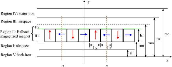
Model of filling air in region II1 and setting Mx = 0.

Thirdly, by using the method mentioned above, the region II1 is filled with air, and set the permanent magnet x-direction magnetization Mx = 0 in region II2, that is to say, it can be regarded as dividing region II1 into region I. Therefore, region II1 is solved using the Laplace equation, and region II2 is solved using the Poisson equation of the quasi-Halbach array. This region II1 filled air model is shown in Fig. 6, and the boundary conditions required for solving the differential equation in this model are Eqs (16) and (27)–(31). $\begin{eqnarray}\displaystyle \text{} & \text{} & \displaystyle \left.A_{II1}\right|_{y=rmi+h1}=\left.A_{II2}\right|_{y=rmi+h1}\end{eqnarray}$ (27) $\begin{eqnarray}\displaystyle \text{} & \text{} & \displaystyle \left.{\displaystyle \frac{1}{{\mu}_{rII1}{\mu}_{0}}}{\displaystyle \frac{\partial A_{II1}}{\partial y}}\right|_{y=rmi+h1}={\displaystyle \frac{1}{{\mu}_{rII2}}}\left({\displaystyle \frac{1}{{\mu}_{0}}}{\displaystyle \frac{\partial A_{II2}}{\partial y}}\left.-0\right)\right|_{y=rmi+h1}\end{eqnarray}$ (28) $\begin{eqnarray}\displaystyle \text{} & \text{} & \displaystyle \left.A_{II2}\right|_{y=rmo}=\left.A_{III}\right|_{y=rmo}\end{eqnarray}$ (29) $\begin{eqnarray}\displaystyle \text{} & \text{} & \displaystyle \left.{\displaystyle \frac{1}{{\mu}_{rIII}{\mu}_{0}}}{\displaystyle \frac{\partial A_{III}}{\partial y}}\right|_{y=rmo}={\displaystyle \frac{1}{{\mu}_{rII2}}}\left(\left.{\displaystyle \frac{1}{{\mu}_{0}}}{\displaystyle \frac{\partial A_{II2}}{\partial y}}-0\right)\right|_{y=rmo}\end{eqnarray}$ (30) $\begin{eqnarray}\displaystyle \text{} & \text{} & \displaystyle \left.H_{II1x}\right|_{y=rmi}=0\end{eqnarray}$ (31)

Using equations (10) and (11), the boundary condition Eqs (16) and (27)–(31) are simplified to obtain Eqs (25) and (32)–(36). $\begin{eqnarray} \displaystyle \text{} & \text{} & \displaystyle A_{In}\cosh k_{n}(rmi+h1)+B_{In}\sinh k_{n}(rmi+h1)=A_{IIn}\cosh k_{n}(rmi+h1)\nonumber\\ \displaystyle \text{} & \text{} & \displaystyle \qquad +∼B_{IIn}\sinh k_{n}(rmi+h1)+{\mu}_{0}{\displaystyle \frac{4Moy}{k_{n}^{2}{\tau}}}\sin {\displaystyle \frac{k_{n}{\tau}}{2}}\sin {\displaystyle \frac{k_{n}Ly}{2}} \end{eqnarray}$ (32) $\begin{eqnarray} \displaystyle \text{} & \text{} & \displaystyle {\displaystyle \frac{1}{{\mu}_{rI}{\mu}_{0}}}(A_{In}k_{n}\sinh k_{n}(rmi+h1)+B_{In}k_{n}\cosh k_{n}(rmi+h1))\nonumber\\ \displaystyle \text{} & \text{} & \displaystyle \qquad =∼{\displaystyle \frac{1}{{\mu}_{rII}}}{\displaystyle \frac{1}{{\mu}_{0}}}(A_{IIn}k_{n}\sinh k_{n}(rmi+h1)+B_{IIn}k_{n}\cosh k_{n}(rmi+h1))-0 \end{eqnarray}$ (33) $\begin{eqnarray} \displaystyle \text{} & \text{} & \displaystyle A_{IIIn}\cosh k_{n}rmo+B_{IIIn}\sinh k_{n}rmo=A_{IIn}\cosh k_{n}rmo\nonumber\\ \displaystyle \text{} & \text{} & \displaystyle \quad +∼B_{IIn}\sinh k_{n}rmo+{\mu}_{0}{\displaystyle \frac{4Moy}{k_{n}^{2}{\tau}}}\sin {\displaystyle \frac{k_{n}{\tau}}{2}}\sin {\displaystyle \frac{k_{n}Ly}{2}} \end{eqnarray}$ (34) $\begin{eqnarray} \displaystyle \text{} & \text{} & \displaystyle {\displaystyle \frac{1}{{\mu}_{rIII}{\mu}_{0}}}(A_{IIIn}k_{n}\sinh k_{n}rmo+B_{IIIn}k_{n}\cosh k_{n}rmo)\nonumber\\ \displaystyle \text{} & \text{} & \displaystyle \quad ={\displaystyle \frac{1}{{\mu}_{rII2}}}{\displaystyle \frac{1}{{\mu}_{0}}}(A_{IIn}k_{n}\sinh k_{n}rmo+B_{IIn}k_{n}\cosh k_{n}rmo)-0 \end{eqnarray}$ (35) $\begin{eqnarray} \displaystyle \text{} & \text{} & \displaystyle A_{In}k_{n}\sinh k_{n}rmi+B_{In}k_{n}\cosh k_{n}rmi=0 \end{eqnarray}$ (36)

The Eqs (25) and (32)–(36) are grouped into a set of equations, and the equations are solved to obtain the value of the coefficient A _IIIn, B _IIIn. Then the A _IIIn, B _IIIn value is substituted into the Eq. (10), and the magnetic potential $A_{III}^{II2}$ value of the region III can be obtained.

Finally, according to the previous assumption, since the components of the magnetic field in the Cartesian coordinate system can be expressed by Eqs (37)–(40), the magnetic flux density from the permanent-region II to the air gap region III can be obtained by the superposition principle. And the equations are (41) and (42). $\begin{eqnarray}\displaystyle \text{} & \text{} & \displaystyle B_{IIIx}^{II1}={\displaystyle \frac{dA_{III}^{II1}}{dy}}\end{eqnarray}$ (37) $\begin{eqnarray}\displaystyle \text{} & \text{} & \displaystyle B_{IIIx}^{II2}={\displaystyle \frac{dA_{III}^{II2}}{dy}}\end{eqnarray}$ (38) $\begin{eqnarray}\displaystyle \text{} & \text{} & \displaystyle B_{IIIy}^{II1}=-{\displaystyle \frac{dA_{III}^{II1}}{dx}}\end{eqnarray}$ (39) $\begin{eqnarray}\displaystyle \text{} & \text{} & \displaystyle B_{IIIy}^{II2}=-{\displaystyle \frac{dA_{III}^{II2}}{dx}}\end{eqnarray}$ (40) $\begin{eqnarray}\displaystyle \text{} & \text{} & \displaystyle B_{IIIx}=B_{IIIx}^{II1}+B_{IIIx}^{II2}\end{eqnarray}$ (41) $\begin{eqnarray}\displaystyle \text{} & \text{} & \displaystyle B_{IIIy}=B_{IIIy}^{II1}+B_{IIIy}^{II2}\end{eqnarray}$ (42)

3. Verification

A virtual Halbach analytical method has been deduced in the previous section. This analysis is mainly to analyze the square quasi-Halbach topology with different heights of main and auxiliary magnetic poles. In this section, a commercial finite element analysis software is used to verify the correctness of this analytical method, using the structural model parameters shown in Table 1. The magnetic flux lines are presented in Fig. 7. In this section, this model is extended to be able to investigate the influence of 𝛼 and 𝛽 on the flux density as shown in Fig. 6. Where, 𝛼 is the ratio of the height of the auxiliary magnetic pole to the height of the main magnetic pole and expressed as Eq. (43), and 𝛽 is the ratio of the length of the auxiliary magnetic pole to the pole pitch and expressed as Eq. (44). $\begin{eqnarray}\displaystyle \text{} & \text{} & \displaystyle {\alpha}=h1/(rmo-rmi)\end{eqnarray}$ (43) $\begin{eqnarray}\displaystyle \text{} & \text{} & \displaystyle {\beta}=Lx/{\tau}\end{eqnarray}$ (44)

Table 1

Parameters of the modeled actuator

Symbol (Unit)	Parameter	Value
ro (mm)	Inner stator height	100
rmo (mm)	Outer magnet height	90
rmi (mm)	Inner magnet height	80
ri (mm)	Inner magnetic barrier height	70
h1 (mm)	Auxiliary magnetic pole permanent magnet height	8
τ (mm)	Pole pitch	20
Lx (mm)	Auxiliary magnetic pole magnetization length	10
B _rx (T)	Remanent flux density ferrite PM	0.4
B _ry (T)	Remanent flux density NdFeB PM	1.1
μ_rNdFeB	Relative permeability NdFeB PM	1.05
μ_rFerrite	Relative permeability ferrite PM	1.05

Fig. 7.

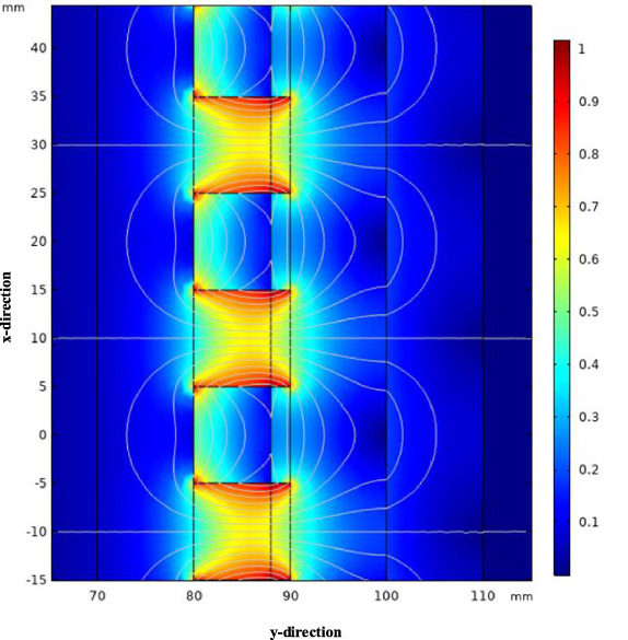
Magnetic flux lines.

The formulas (41) and (42) for the air field in region III will be verified by comparing to a finite element analysis (FEA). The permanent magnets in the FEA model have a remanent flux density, B _rNdFeB = 1. 1T, B _rFerrite = 0. 4T and the relative permeability, μ_rII1 = μ_rNdFeB = μ_rFerrite. It can be seen from Fig. 8 that the absolute value of the maximum error of the y component flux density between the analytical solution and the finite element solution is 0.0138T, which occurs at x = 29.5 mm and B _IIIy = −0.4631T; and the absolute maximum error of x component flux density is 0.0212T, which occurs at x = 16.34 mm and B _IIIx = 0.3792T. It can be obtained from Fig. 9 that the absolute value of the maximum error of the y component flux density between the analytical solution and the finite element solution is 0.0149T, which occurs at x = 9.96 mm and B _IIIy = 0.4093T; and The absolute maximum error of x component flux density is 0.0196T, which occurs at x = 21.39 mm and B _IIIx = 0.2749T. Therefore, in the air gap magnetic field along the line y = 91 and y = 92, the analytical solution agrees well with the B _IIIx and B _IIIy waveform of the finite element solution in one cycle, the waveform trend is very consistent, and the error between the two is very small. Obviously, the results show match well for the air field along the line y = 91 and y = 92 mm for 0 < x < 40 mm, and the virtual Halbach analytical method gives a slightly stronger field, due to the approximation μ_rII ≈ 1.

Fig. 8.

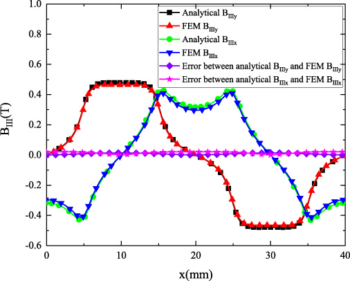
Comparison of the x and y component of the air field flux density calculated by analytical means and FEM along the line y = 91 mm for 0 < x < 40 mm.

Fig. 9.

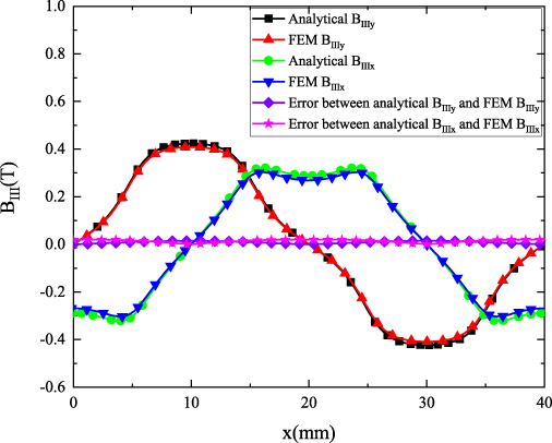
Comparison of the x and y component of the air field flux density calculated by analytical means and FEM along the line y = 92 mm for 0 < x < 40 mm.

4. Results

This paper firstly investigates the two parameter variations of the shape of the magnetic pole, one is the ratio of the auxiliary magnetic pole to the magnetization direction of the main magnetic pole, and the other is the ratio of the auxiliary magnetic pole to the pole pitch in the x direction. To evaluate the effect of changing the magnet shape, the field distribution in the center of region III is calculated for several values of 𝛼 and 𝛽. By optimizing the two-segment quasi-Halbach topology actuator model, the maximum value of the first harmonic air gap flux density can be obtained with unequal heights and unequal lengths of the main and auxiliary magnetic poles, and the effect of changes in 𝛼 and 𝛽 on the peak value of the air gap can also be obtained. Fig. 10 shows an analytical model result waveform of five different alpha values, where 𝛼 = 1 corresponds to the case where the square quasi-Halbach topology main magnetic pole and the auxiliary magnetic pole are highly equal in the magnetization direction, that is, the traditional two-segment quasi-Halbach mode shown in Fig. 2. As shown in the figure, when the 𝛼 value changes from 0.5 to 0.98, the peak value of the waveform also corresponds to an incremental change, and the peak value of the waveform for 𝛼 = 0.98 is higher. Fig. 11 shows the analytical model result waveforms for five different beta values, where 𝛽 = 0.5 corresponds to the case where the Halbach main magnetic pole and the auxiliary magnetic pole are equal in length in the x direction. As shown in the figure, when the 𝛽 value changes from 0.3 to 0.6, the peak value of the waveform also corresponds to an incremental change, and the peak value of the waveform for 𝛽 = 0.6 is higher.

At the same time, this paper also investigates the influence of the variation of residual magnetic flux density on the air gap magnetic density. Since the auxiliary magnetic pole adopts a low coercivity ferrite material, and the residual magnetic density of the different types of ferrite after saturation magnetization generally has a range of 0.2–0.44 T, it is very meaningful to examine the effect of this parameter on the air gap flux density. Figure 12 shows the analytical model waveforms for six different B _rx values, where B _rx = 0.2 and B _rx = 0.44 correspond to the minimum and maximum remanence of the auxiliary pole ferrite of the square Halbach structure, respectively. As shown in the figure, when the B _rx value changes from 0.2 to 0.44, the peak value of the waveform also corresponds to an incremental change, and the peak value of the waveform for B _rx = 0.44 is higher.

Fig. 10.

Effect of 𝛼 on the waveform of the y component of the flux density along the line y = 91.5 mm for 0 < x < 40 mm in the region III.

Fig. 11.

Effect of 𝛽 on the waveform of the y component of the flux density along the line y = 91.5 mm for 0 < x < 40 mm in the region III.

Fig. 12.

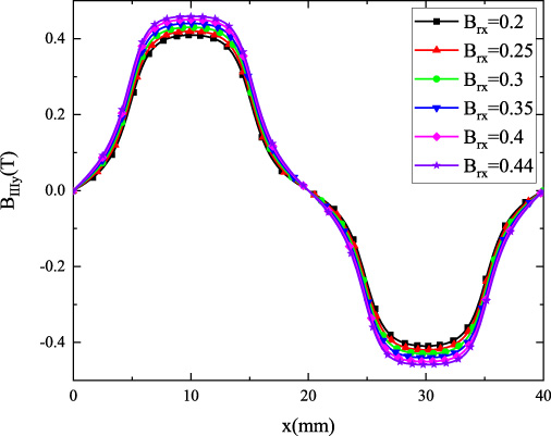
Effect of B _rx on the waveform of the y component of the flux density along the line y = 91.5 mm for 0 < x < 40 mm in the region III.

However, it can be seen from the influence of the changes of the parameters 𝛼, 𝛽 and B _rx on the air gap magnetic density that the different parameter 𝛼 and 𝛽 parameter values correspond to different magnetic density waveforms. In order to evaluate the air gap magnetic density waveform of the quasi-Halbach topology, it is necessary to calculate the total harmonic distortion (THD _B) in y direction, that is, the ratio of the root mean square value of the harmonic content of all air gap magnetic fields to the root mean square value of the fundamental wave, as shown in the following formula (45). $\begin{eqnarray} \displaystyle THD_{By}={\displaystyle \frac{\sqrt{\mathop{\displaystyle\sum }_{n=2}^{\infty }B_{yn}^{2}}}{B_{y1}}}. & & \displaystyle \end{eqnarray}$ (45)

Where, THD _By is the harmonic total distortion rate of the y-direction flux density waveform, B _y1 is the fundamental component of the flux density, and B _yn is the nth harmonic component of the flux density.

Using the Eq. (45) to process the waveforms in Fig. 10, Fig. 11, and Fig. 12, the THD _B values corresponding to the different 𝛼, 𝛽 and B _rxvalues can be obtained, as shown in Table 2. The different 𝛼 values in Table 2 correspond to different harmonic distortion rates. The maximum THD _By value at 𝛼 = 0.7 is 0.1885, and the minimum THD _By value at 𝛼 = 0.9 is 0.1589. It is shown that the harmonic minimum occurs where the height of the main and auxiliary magnetic poles is different, and the magnetic density waveform of the quasi-Halbach permanent magnet obtains better performance. The maximum THD _By value at 𝛽 = 0.3 is 0.3451, and the minimum THD _By value at 𝛽 = 0.55 is 0.1457. It is shown that the harmonic minimum occurs where the auxiliary magnetic pole length is slightly larger than the main magnetic pole length, and the magnetic flux waveform of the permanent magnet obtains better performance. The minimum THD _By value at remanence of auxiliary magnetic pole B _rx = 0.2T is 0.1514, and the maximum THD _By value at remanence of auxiliary magnetic pole B _rx = 0.4T is 0.1724. It shows that the residual magnetism of the auxiliary magnetic pole also affects the magnetic flux density waveform of the permanent magnet air gap. Therefore, as can be seen from the previous discussion, the changes of the three parameters 𝛼, 𝛽 and B _rx have an effect on the air gap magnetic density waveform.

Table 2

Effect of THD on the waveform of 𝛼, 𝛽 and B _rx

Parameter	Value	Parameter	Value	Parameter	Value
THD _By for 𝛼 = 0.5	0.1764	THD _By for 𝛽 = 0.3	0.3451	THD _By for B _rx = 0.2	0.1514
THD _By for 𝛼 = 0.7	0.1885	THD _By for 𝛽 = 0.45	0.1818	THD _By for B _rx = 0.25	0.1544
THD _By for 𝛼 = 0.8	0.1694	THD _By for 𝛽 = 0.5	0.1470	THD _By for B _rx = 0.3	0.1595
THD _By for 𝛼 = 0.9	0.1589	THD _By for 𝛽 = 0.55	0.1457	THD _By for B _rx = 0.35	0.1527
THD _By for 𝛼 = 0.98	0.1724	THD _By for 𝛽 = 0.6	0.1623	THD _By for B _rx = 0.4	0.1724

5. Conclusions

This paper proposes a new virtual Halbach analytical method for permanent magnet slotless planar linear actuators having mixed high-coercivity NdFeB magnets and low-coercivity ferrite magnets to form a two-segment quasi-Halbach topology with different heights of main and auxiliary magnetic poles, and the three-parameter 𝛼, 𝛽 and B _rx, which is closely related to the shape of the magnetic pole and the magnetic flux density, is used to optimize the Halbach magnetized permanent magnet topology with this analytical method. Firstly, the analytical model for the shaped magnetic pole of slotless planar linear actuator is established, and the virtual Halbach analytical method is derived to optimize the Halbach topology. Then, the analytic method is verified by the finite element method. From the perspective of the magnetic density waveform, the results agree well. Finally, the actuator topology is optimized by three parameters in the analytical method. It is concluded that the three parameters 𝛼, 𝛽 and B _rx have a great influence on the air gap flux density waveform. Analysis shows that the magnetic distortion waveform has the smallest harmonic distortion rate where 𝛼 = 0.9, 𝛽 = 0.55 and B _rx = 0.2. However, additional research using the analytical method presented in this paper is necessary as the desired air-gap flux density waveform strongly depends on the planar linear actuator Halbach topology with the different heights of main and auxiliary magnetic poles.

Footnotes

Acknowledgements

This work was funded by a project that partially funded by National Science Foundation of China (51675265) and the Priority Academic Program Development of Jiangsu Higher Education Institutions (PAPD). The authors gratefully acknowledge this support.

References

Wang

Howe

and Jewell

G.W.

, Fringing in tubular permanent-magnet machines: Part II. Cogging force and its minimization, IEEE Transactions on Magnetics 39(2003) 3517–3522.

Shen

and Zhu

Z.Q.

, Analysis of electromagnetic performance of Halbach PM brushless machines having mixed grade and unequal height of magnets, IEEE Transactions on Magnetics 49(2013) 1461–1469.

Huang

Jing

and Li

, Analysis and application of discrete Halbach magnet array with unequal arc lengths and unequally changed magnetization directions, IEEE Transactions on Applied Superconductivity 28(2018) 5201305.

Jiao

Wang

and Liang

, Design of a tubular linear oscillating motor with novel compound Halbach magnet array, IEEE-ASME Transactions on Mechatronics 22(2017) 498–508.

and Feng

, Analysis on toothless permanent magnet machine with Halbach array, in: 2006 CES/IEEE 5th International Power Electronics and Motion Control Conference, IPEMC, 2006, pp. 1–5.

Zhu

Z.Q.

and Howe

, Halbach permanent magnet machines and applications: A review, IEE Proceedings Electric Power Applications 148(2001) 299–308.

Halbach

, Design of permanent multipole magnets with oriented rare earth cobalt material, Nuclear Instruments and Methods 169(1980) 1–10.

Tiang

T.L.

Ishak

Lim

C.P.

and Kamarol

, A novel analytical method using virtual PM blocks to optimize magnet segmentations in surface-mounted PM synchronous machines, in: 2015 International Conference on Electrical Machines and Systems, ICEMS, 2015, pp. 1278–1283.

Dai

Cao

Long

Liang

and Wang

, Analytical modeling of an eddy-current adjustable-speed coupling system with a three-segment Halbach magnet array, Electric Machines and Power Systems 43(2015) 1891–1901.

10.

Xia

Guo

and Wang

, Modeling and analyzing of magnetic field of segmented Halbach array permanent magnet machine considering gap between segments, IEEE Transactions on Magnetics 50(2014) 1–9.

11.

Ashabani

and Mohamed

A.R.I.

, Multiobjective shape optimization of segmented pole permanent-magnet synchronous machines with improved torque characteristics, IEEE Transactions on Magnetics 47(2011) 795–804.

12.

Isfahani

A.H.

, Analytical framework for thrust enhancement in permanent-magnet (PM) linear synchronous motors with segmented PM poles, IEEE Transactions on Magnetics 46(2010) 1116–1122.

13.

Markovic

and Perriard

, Optimization design of a segmented Halbach permanent-magnet motor using an analytical model, IEEE Transactions on Magnetics 45(2009) 2955–2960.

14.

Lee

M.G.

and Gweon

D.G.

, Optimal design of a double-sided linear motor with a multi-segmented trapezoidal magnet array for a high precision positioning system, J. Magn. Magn. Mater. 281(2004) 336–346.

15.

Wang

Chen

and Wu

, Research on analytical model and design formulas of permanent magnetic bearings based on Halbach array with arbitrary segmented magnetized angle, J. Magn. Magn. Mater. 410(2016) 257–264.

16.

Hogberg

Pedersen

T.S.

Bendixen

F.B.

Mijatovic

and Holboll

, Direct reuse of rare earth permanent magnets - wind turbine generator case study, in: 2016 XXII International Conference on Electrical Machines, ICEM, 2016, pp. 1625–1629.

17.

and Zhu

Z.Q.

, Analytical modeling of surface-mounted PM machines accounting for magnet shaping and varied magnet property distribution, IEEE Transactions on Magnetics 50(2014) 1–11.

18.

Hong

and Yoo

, Shape design of the surface mounted permanent magnet in a synchronous machine, IEEE Transactions on Magnetics 47(2011) 2109–2117.

19.

Laskaris

K.I.

and Kladas

A.G.

, Permanent-magnet shape optimization effects on synchronous motor performance, IEEE Transactions on Industrial Electronics 58(2011) 3776–3783.

20.

Tavana

N.R.

and Shoulaie

, Analysis and design of magnetic pole shape in linear permanent-magnet machine, IEEE Transactions on Magnetics 46(2010) 1000–1006.

21.

Yong

Zhu

Z.Q.

and Feng

Z.J.

, Cogging torque in cost-effective surface-mounted permanent-magnet machines, IEEE Transactions on Magnetics 47(2011) 2269–2276.

22.

Meessen

K.J.

Gysen

Paulides

and Lomonova

E.A.

, Halbach permanent magnet shape selection for slotless tubular actuators, IEEE Transactions on Magnetics 44(2008) 4305–4308.

23.

Zhang

and Li

, Analytical model of magnetic field of a permanent magnet synchronous motor with a trapezoidal Halbach permanent magnet array, IEEE Transactions on Magnetics 99(2019) 1–5.

24.

Duan

Song

and Zhang

, A novel 3-D analytical modeling method of trapezoidal shape permanent magnet Halbach array for multi-objective optimization, Journal of Electrical Engineering and Technology 14(2019) 635–643.

25.

Isfahani

A.H.

Vaez-Zadeh

and Rahman

M.A.

, Performance improvement of permanent magnet machines by modular poles, IET Electric Power Applications 3(2009) 343–351.

26.

Isfahani

A.H.

Vaez-Zadeh

and Rahman

M.A.

, Using modular poles for shape optimization of flux density distribution in permanent-magnet machines, IEEE Transactions on Magnetics 44(2008) 2009–2015.

27.

Liu

and Wang

, Magnetic field analysis and optimisation of permanent magnet machines with novel two-segment Halbach array, IET Electric Power Applications 13(2019) 1355–1364.

28.

Zhu

Z.Q.

L.J.

and Xia

Z.P.

, An accurate subdomain model for magnetic field computation in slotted surface-mounted permanent-magnet machines, IEEE Transactions on Magnetics 46(2010) 1100–1115.

29.

Jin

Yuan

and Lin

, General analytical method for magnetic field analysis of halbach magnet arrays based on magnetic scalar potential, Journal of Magnetics 18(2013) 95–104.

30.

Sun

R.X.

Deng

Z.G.

Gou

Y.F.

Y.J.

Zheng

Wang

S.Y.

and Wang

J.S.

, Feasibility of low-cost magnetic rail designs by integrating ferrite magnets and NdFeB magnets for HTS Maglev systems, International Journal of Modern Physics B 29(2015) 1542043.

31.

Sun

Zheng

Qian

and Deng

, New magnetic rails with double-layer Halbach structure by employing NdFeB and ferrite magnets for HTS maglev, J. Magn. Magn. Mater. 445(2018) 44–48.

32.

Wang

and Zheng

, Analytical predictions and analysis of electromagnetic field and torque for eddy-current couplers with Quasi-Halbach magnet array, International Journal of Applied Electromagnetics and Mechanics 57(2018) 347–366.

33.

Jang

Koo

and Kim

, Torque characteristic analysis and measurement of axial flux-type non-contact permanent magnet device with Halbach array based on 3D analytical method, AIP advances 7(2017) 0566475.

34.

Koo

Choi

Shin

and Kim

, No-load analysis of PMLSM with Halbach array and pm overhang based on three-dimensional analytical method, IEEE Transactions on Applied Superconductivity 26(2016) 0604905.

35.

Mallek

Tang

and Lee

, An analytical subdomain model of torque dense Halbach array motors, Energies 11(2018) 3254.