An exact analysis for heat conduction in laminated infinite cylindrical arches subjected to Dirichlet boundary conditions

Abstract

The temperature field within a layered arch subjected to Dirichlet Boundary Conditions is investigated based on the exact heat conduction theory. An analytical method is shown to obtain the temperature field in the arch. Because of the complex of the temperature boundary conditions, the temperature field is divided into two parts with the linear superposition principle. The first part is a temperature filed from the temperature boundary conditions on the lateral surfaces. The second part is from the temperature conditions on the outside surfaces expect the influence from the two edges. The temperature solution of the first part is constructed directly according to the temperature boundary conditions on the lateral surfaces. The temperature solution of the second part is studied with transfer matrix method. The convergence of the solutions is checked with respect to the number of the terms of series. Comparing the results with those obtained from the finite element method, the correctness of the present method is verified. Finally, the influences of surface temperature and the thickness-radius ratio h∕r₀ on the distribution of temperature in the arch are discussed in detail.

Keywords

Layered arch heat conduction theory temperature the transfer matrix Dirichlet boundary conditions

1. Introduction

The mechanical properties of layered arches subjected to thermal loads have received a considerable attention. Because of the inhomogeneity of thermal expansion coefficients in different layers, the stresses and non-uniform deformations appear even for a completely free layered arch. Therefore, the study to temperature distribution of layered arches has particular importance for structural safety analysis.

A lot of researches on the distribution of temperature in the laminates were reported. Ostrowski and Jędrysiak [1] studied heat conduction in a two-phase laminate made of periodically distributed micro-laminas along one direction. Vidal et al. [2] computed explicit thermal solutions for laminated and sandwich beams with arbitrary heat source location. Kantor et al. [3] present a method for determination of thermal condition of laminated elements of structures. Based on the immersion method, Shupikov et al. [4] showed an analytical solution for the problem of nonstationary heat conduction in laminated plates of complex plan shape when they are heated with interlayer film heat sources. Kayhani et al. [5] present an exact solution for steady-state conduction heat transfer in cylindrical composite laminates. Abdelal et al. [6] studied the effect of steering fibers on transient heat conduction under uniform heat flux. Matysiak and Perkowski [7] present the distributions of temperature and heat fluxes in a periodically laminated layer with a vertically located cylindrical hole. Tarn and Wang [8] studied heat conduction in circular cylinders of functionally grad-ed materials and laminated composites by means of matrix algebra and eigenfunction expansion. Nemirovskii and Yankovskii [9] present a method of asymptotic expansions of the solutions of the steady heat conduction problem for laminated non-uniform anisotropic plates. Kulikov and Plotnikova [10] used the method of sampling surfaces to analyze the exact three-dimensional heat conduction of laminated orthotropic and anisotropic shells. Mityushev et al. [11] described a method of heat conduction in various type of composite materials. Delouei et al. [12] presented an exact analytical solution for transient heat conduction in cylindrical multi-layered composites. Kayhani et al. [13] presented a steady analytical solution for heat conduction in a cylindrical multilayered laminate with different steady analytical solution for heat conduction in a cylindrical multilayered laminate with different fiber directions among layers. The Sturm-Liouville theorem was used to derive the appropriate Fourier transformation. Ma and Chang [14] analyzed the steady-state temperature field and heat flux field in a multi-layered media with anisotropic properties subjected to surface temperature.

2. Basic equations

In this paper, the exact heat conduction theory is used to study the steady temperature distribution in a layered arch subjected to Dirichlet Boundary Conditions. A laminated infinite cylindrical arch with radius r_i (i = 1,2…p) and the angle θ₀ of the arch is considered, as shown in Fig. 1. The inner radius is r₀. The arch is composited of p isotropic layers with non-uniform thickness. The thermal conductivity of the ith layer is k_i. We consider the arch keeping two different constant temperatures on two edges, respectively. The temperature value at the θ = 0 edge is taken as the datum mark of the temperature field in the arch. Without losing the generality we can further consider the temperatures on the left edge to be zero. So, the constant temperature at the θ = θ₀ edge is t_r. The outermost surface and the innermost surface are subjected to temperatures load t_p(θ) and t₁(θ), respectively. We assume that the changes of material properties don’t occur under the temperature loads.

Fig. 1.

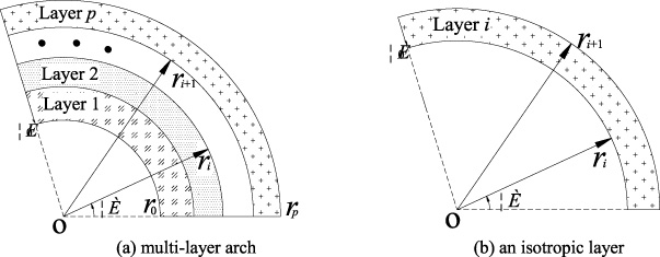
Model of the layered arch.

Due to the complex of the temperature field in the laminated arch, the temperature solution can be divided into two parts based on the linear superposition principle. The first part is a temperature filed from the temperature boundary conditions on the lateral surfaces. The second part is from the temperature conditions on the outside surfaces expect the influence from the two edges. Further, the temperature boundary conditions on the two edges can be set to zero in this part.

2.1. The temperature solution of the first part

Now, an arbitrary layer in the layered arch such as the ith layer is considered in Figure 1(b). In the polar coordinates system r − θ, the heat conduction equation in the ith isotropic layer is $\begin{eqnarray}\displaystyle {\displaystyle \frac{\partial ^{2}T_{i}(r,{\theta})}{\partial r^{2}}}+{\displaystyle \frac{1}{r}}{\displaystyle \frac{\partial T_{i}(r,{\theta})}{\partial r}}+{\displaystyle \frac{1}{r^{2}}}{\displaystyle \frac{\partial ^{2}T_{i}(r,{\theta})}{\partial {\theta}^{2}}}=0 & & \displaystyle\end{eqnarray}$ (1) where T_i(r, θ) is the temperature distribution in the ith layer.

The temperature conditions on two edges of the laminated arch can be written as follows, $\begin{eqnarray}\displaystyle T_{i}(r,0)=0,\quad T_{i}(r,{\theta}_{0})=t_{r}. & & \displaystyle\end{eqnarray}$ (2) From the temperature Dirichlet Boundary Conditions, the temperature solution of the first part can be constructed as $\begin{eqnarray}\displaystyle T_{1i}(r,{\theta})={\displaystyle \frac{t_{r}}{{\theta}_{0}}}{\theta}. & & \displaystyle\end{eqnarray}$ (3)

It is obvious that the temperature solution (3) satisfies the temperature boundary conditions exactly.

2.2. The temperature solution of a layer in the second part

The temperature boundary conditions in the second part are $\begin{eqnarray}\displaystyle T_{2i}(r,0)=0,\quad T_{2i}(r,{\theta}_{0})=0. & & \displaystyle\end{eqnarray}$ (4) The solution of Eq. (1) can be given in the sinusoidal series form of $\begin{eqnarray}\displaystyle T_{2i}(r,{\theta})=\displaystyle \mathop{\sum }_{m=1}^{\infty }t_{mi}(r)\sin ({\beta}_{m}{\theta}) & & \displaystyle\end{eqnarray}$ (5) where, ${\beta}_{m}=\frac{m{\pi}}{{\theta}_{0}}$ .

It is obvious that Eq. (5) satisfies Eq. (4) exactly. Substituting general temperature solution (5) into Eq. (1), T₂_i(r, θ) can be worked out: $\begin{eqnarray}\displaystyle T_{2i}(r,{\theta})=\displaystyle \mathop{\sum }_{m=1}^{\infty }[r^{{\beta}_{m}}E_{mi}+r^{-{\beta}_{m}}F_{mi}]\sin ({\beta}_{m}{\theta}) & & \displaystyle\end{eqnarray}$ (6) where, E_mi and F_mi are the unknown functions, which can be determined by the temperature conditions on the inner and outer surfaces of the ith layer.

3. Recursive formulae

The relationships of the temperature and the heat flux on the interface of two adjacent layers with different thermal conductivities are $\begin{eqnarray}\displaystyle T_{2(i+1)}(r_{i},{\theta})=T_{2i}(r_{i},{\theta}),\quad \left.k_{i+1}{\displaystyle \frac{\partial T_{2(i+1)}(r_{i},{\theta})}{\partial r}}\right|_{r=r_{i}}=\left.k_{i}{\displaystyle \frac{\partial T_{2i}(r,{\theta})}{\partial r}}\right|_{r=r_{i}}. & & \displaystyle\end{eqnarray}$ (7) From Eq. (6), the temperature and heat flux in the ith layer can be written in the form of matrix, i.e. $\begin{eqnarray}\displaystyle \left[\begin{array}{@{}c@{}}T_{2i}(r,{\theta})\\ k_{i}{\displaystyle \frac{\partial T_{2i}(r,{\theta})}{\partial r}}\\ \end{array}\right]=\displaystyle \mathop{\sum }_{m=1}^{\infty }\sin ({\beta}_{m}{\theta})[{\phi}_{mi}(r)] & & \displaystyle\end{eqnarray}$ (8) where [𝜙_mi(r)] is the matrix function of r with unknown coefficients.

According to Eq. (6), [𝜙_mi(r)] can be expressed as $\begin{eqnarray}\displaystyle [{\phi}_{mi}(r)]=[{\varphi}_{mi}(r)][{\Lambda}_{mi}] & & \displaystyle\end{eqnarray}$ (9) in which, [φ_mi(r)] and [𝛬_mi] are $\begin{eqnarray}\displaystyle [{\varphi}_{mi}(r)]=\left[\begin{array}{@{}cc@{}}r^{{\beta}_{m}} & r^{-{\beta}_{m}}\\ k_{i}{\beta}_{m}r^{{\beta}_{m}-1} & -k_{i}{\beta}_{m}r^{-{\beta}_{m}-1}\end{array}\right],\quad [{\Lambda}_{mi}]=\left[\begin{array}{@{}c@{}}E_{mi}\\ F_{mi}\end{array}\right]. & & \displaystyle\end{eqnarray}$ (10)

The continuity of the temperature and heat flux at the interface can be expressed as $\begin{eqnarray}\displaystyle [{\phi}_{mi}(r_{i})]=[{\phi}_{m(i+1)}(r_{i})]. & & \displaystyle\end{eqnarray}$ (11) Thus, the temperature and heat flux relationships between the layer q (q = 2, 3…p) and innermost layer of the arch are recursively obtained: $\begin{eqnarray}\displaystyle [{\Lambda}_{mq}]=[{\varphi}_{mq}(r_{q})]^{-1}\left\{\displaystyle \mathop{\prod }_{j=q}^{1}[{\varphi}_{mj}(r_{j})][{\varphi}_{mj}(r_{j-1})]^{-1}\right\}[{\varphi}_{m1}(r_{0})][{\Lambda}_{m1}]. & & \displaystyle\end{eqnarray}$ (12)

4. Unknown coefficients

Consider that the outermost and innermost surfaces of the layered arch are subjected to the steady state temperature loads t_p(θ) and t₁(θ) respectively, i.e. $\begin{eqnarray}\displaystyle T_{1}(r_{0},{\theta})=t_{1}({\theta}),\quad T_{p}(r_{p},{\theta})=t_{p}({\theta}). & & \displaystyle\end{eqnarray}$ (13) The temperature boundary conditions in the second part can be derived out as follows, $\begin{eqnarray}\displaystyle T_{20}(r_{0},{\theta})=t_{1}({\theta})-T_{10}\left(r_{0},{\theta}\right),\quad T_{2p}(r_{p},{\theta})=t_{p}({\theta})-T_{1p}\left(r_{p},{\theta}\right). & & \displaystyle\end{eqnarray}$ (14)

Substituting Eq. (6) into the above equation, then multiplying Eq. (14) by $\sin \left(\frac{i{\pi}}{{\theta}_{0}}{\theta}\right)$ and integrating over θ, gives: $\begin{eqnarray}\displaystyle \begin{array}{@{}l@{}}\displaystyle \int _{0}^{{\theta}_{0}}T_{20}(r_{0},{\theta})\sin \left({\displaystyle \frac{i{\pi}}{{\theta}_{0}}}{\theta}\right)d{\theta}=\displaystyle \int _{0}^{{\theta}_{0}}[t_{1}({\theta})-T_{10}(r_{0},{\theta})]\sin \left({\displaystyle \frac{i{\pi}}{{\theta}_{0}}}{\theta}\right)d{\theta},\\[12.0pt] \displaystyle \int _{0}^{{\theta}_{0}}T_{2p}(r_{p},{\theta})\sin \left({\displaystyle \frac{i{\pi}}{{\theta}_{0}}}{\theta}\right)d{\theta}=\displaystyle \int _{0}^{{\theta}_{0}}[t_{p}({\theta})-T_{1p}(r_{p},{\theta})]\sin \left({\displaystyle \frac{i{\pi}}{{\theta}_{0}}}{\theta}\right)d{\theta}.\end{array} & & \displaystyle\end{eqnarray}$ (15)

Simultaneously solving Eq. ((12)) (taking q = p) and Eq. ((15)), E_m₁, F_m₁, E_mp and F_mp can be uniquely determined. Taking E_m₁ and F_m₁ back to Eq. ((12)), E_mq and F_mq (q = 2,3…p −1) for each layer can be recursively obtained. Finally, substituting the coefficients back into Eq. ((6)) yields the temperature field of the second part. And the temperature solution in the layered arch can be obtained with the first part solution ((3)) and the second part solution ((6)) as follows, $\begin{eqnarray}\displaystyle T_{i}(r,{\theta})=\displaystyle \mathop{\sum }_{m=1}^{\infty }[r^{{\beta}_{m}}E_{mi}+r^{-{\beta}_{m}}F_{mi}]\sin ({\beta}_{m}{\theta})+{\displaystyle \frac{t_{r}}{{\theta}_{0}}}{\theta}. & & \displaystyle\end{eqnarray}$ (16)

5. Convergence and comparison studies

In order to verify the accuracy and correctness of the present method, some numerical calculations for the convergence of temperature solutions are carried out. A three-layer arch is taken as example, which is widely used in various engineering. The outermost and innermost layers of the arch are made up of steel while the core layer is made up of concrete. The radii are r₀ = 0.5 m, r₁ = 0.7 m, r₂ = 0.9 m, r₃ = 1.1 m, respectively. The angle θ₀ of the arch is π∕2. The thermal conductivities for every layer are k₁ = 50 W/(m ⋅ °C), k₂ = 2 W/(m ⋅ °C), k₃ = 50 W/(m ⋅ °C), respectively. The outside surfaces are subjected to uniform steady-state temperature loads: t_p(θ) = 100 °C and t₁(θ) = 20 °C, respectively. The temperature convergence is checked with five different series terms N = 8, 13, 18, 23, 28. Table 1 gives the solutions of temperature at five different points: θ = π∕4, r = 0.6 m, r = 0.7 m, r = 0.8 m, r = 0.9 m, r = 1.0 m, respectively. It can be seen from Table 1 that the numerical results converge quickly with the increase of the series terms. The results for N = 28 have the same three significant figures as those for N = 23. Therefore, the number of terms of the Fourier series is fixed at N = 23 in the following numerical computations.

Meanwhile, a finite element (FE) simulation using ANSYS software (Element: solid 90) has been carried out to verify the correctness of the proposed method. Table 2 gives the comparison studies of temperature solutions at five points, i.e. θ = π∕4 for r = 0.6 m, 0.7 m, 0.8 m, 0.9 m, 1.0 m, respectively. It can be seen from Table 2 that the present solutions agree closely with the FE solution.

Table 1
Convergence of the present method

N r = 0.6 m r = 0.7 m r = 0.8 m r = 0.9 m r = 1.0 m

8 20.3 20.6 57.9 95.3 97.6

13 20.5 21.1 58.3 95.6 97.8

18 20.7 21.4 58.7 96.5 98.2

23 21.2 22.6 61.8 97.1 98.5

28 21.2 22.6 61.8 97.1 98.5

N	r = 0.6 m	r = 0.7 m	r = 0.8 m	r = 0.9 m	r = 1.0 m
8	20.3	20.6	57.9	95.3	97.6
13	20.5	21.1	58.3	95.6	97.8
18	20.7	21.4	58.7	96.5	98.2
23	21.2	22.6	61.8	97.1	98.5
28	21.2	22.6	61.8	97.1	98.5

Table 2

Comparisons with the FE solutions along θ = π∕4

Position	r = 0.6 m	r = 0.7 m	r = 0.8 m	r = 0.9 m	r = 1.0 m
ANSYS	20.1	22.6	61.8	97.1	98.5
Present	21.2	22.6	61.8	97.1	98.5

6. Numerical examples

In this section, the effects of surface temperatures and thickness-radius ratio on the temperature were discussed for two typical cases.

6.1. Effect of different surface temperature

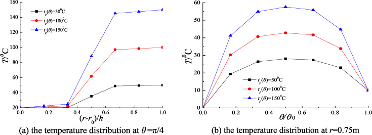
The first example is a three-layer arch. The radii are r₀ = 1 m, r₁ = 1.5 m, r₂ = 2 m, r₃ = 2.5 m, respectively. The angle θ₀ of the arch is π∕2. The outermost surface of the arch is subjected to three different temperature loads: 50 °C, 100 °C, 150 °C respectively. The temperature at the innermost surface of the arch is fixed at 20 °C. The temperature value at the θ = θ₀ edge is t_r = 10 °C.

Figure 2(a) shows the temperature distribution along the r direction at θ = π∕4 for different boundary temperatures. We can find from Fig. 2(a) that the slopes of temperature variations along the r direction in the surface layers are small. However, it is considerable in the core layer is. The reason is that the thermal conductivity in the surface layers is much larger than that in the core layer. Figure 2(b) shows the temperature distribution along the θ direction at r = 0.75 m. It can be found that the temperatures in the same positions increase with the increase of the temperature on the outermost surface of the arch.

Fig. 2.

The temperature distribution under different surface temperatures.

6.2. Effect of different surface temperatures

The second example is the arch of three layers with h = 0.6 m and h₁ = h₂ = h₃ = 0.2 m. The angle θ₀ of the arch is π∕2. Three different arch r₀ are considered: r₀ = 0.5 m, 1 m, 2 m, i.e. h∕r₀ = 1.2, 0.6, 0.3, respectively. The surfaces are subject to the uniform steady-state temperature loads: t_p(θ) =100 °C and t₁(θ) = 20 °C, respectively. The temperature value at the θ = θ₀ edge is t_r = 10 °C. It can be seen from Fig. 3(a) that the temperature distributions are almost the same at θ = π∕4 for different h∕r₀. The temperature distributions along the θ direction at r − r₀ = 0.25 m are plotted in Fig. 3(b). It can be found from Fig. 3(b) that the temperature distribution is asymmetric and the temperatures in the right part are a litter larger than the left part. The reason is that the temperature at the θ = θ₀ edge is larger than θ = 0 edge.

Fig. 3.

The temperature distribution in layered arches of different thickness-radius ratio.

7. Conclusion

The temperature distribution in the layered arch subjected to Dirichlet Boundary Conditions is studied based on the exact heat conduction theory. Main conclusions are summarized as follows:

(1) An exact analytic solution of temperature in the layered arch subjected to Dirichlet Boundary Conditions is present based on the exact heat conduction theory.

(2) Some numerical calculations for the convergence of temperature solutions are carried out. The present method shows an excellent convergence. Comparing the results with those obtained from the finite element method, the correctness of the present method is verified.

(3) The influences of the surface temperatures and the thickness-radius ratio h∕r₀ on the temperature are discussed in detail. It is shown that the temperature in the arch increases with the increase of the surface temperature. The surface temperature and geometric dimensions arch have an important effect on the distributions of the temperature in the layered arches.

Footnotes

Acknowledgements

This work is financially supported by the Research Foundation for Advanced Talents of Jiangsu University (Grant No. 16JDG053), the Natural Science Foundation of Jiangsu Province (Grant No. BK20160519, BK20160534, BK20190833), the National Natural Science Foundation of China (Grant No. 51608234).

Conflict of interest

The authors declared that they have no conflicts of interest to this work.

References

Ostrowski

and Jędrysiak

, Heat conduction in periodic laminates with probabilistic distribution of material properties, Heat Mass Transfer53 (2017), 1425–1437.

Vidal

Gallimard

Ranc

and Polit

, Thermal and thermo-mechanical solution of laminated composite beam based on a variables separation for arbitrary volume heat source locations, Applied Mathematical Modelling46 (2017), 98–115.

Kantor

B.Y.

Smetankina

N.V.

and Shupikov

A.N.

, Analysis of non-stationary temperature fields in laminated strips and plates, Intl J. Solids Struct.38 (2001), 8673–8684.

Shupikov

A.N.

Smetankina

N.V.

and Svet

Y.V.

, Nonstationary heat conduction in complex-shape laminated plates, Journal of Heat Transfer-transactions of the ASME129 (2007), 335–341.

Kayhani

M.H.

Shariati

Nourozi

and Demneh

M.K.

, Exact solution of conductive heat transfer in cylindrical composite laminate, Heat Mass Transfer46 (2009), 83–94.

Abdelal

G.F.

Abdalla

M.M.

and Gurdal

, Transient heat conduction of variable stiffness composite laminate, Journal of Thermal Stresses33 (2010), 121–134.

Matysiak

S.J.

and Perkowski

D.M.

, Axially symmetric problems of heat conduction in a periodically laminated layer with vertical cylindrical hole, International Communications in heat and Mass Transfer38 (2011), 410–417.

Tarn

J.Q.

and Wang

Y.M.

, End effects of heat conduction in circular cylinders of functionally graded materials and laminated composites, Intl J. Heat Mass Transfer47 (2004), 5741–5747.

Nemirovskii

Y.V.

and Yankovskii

A.P.

, A method of asymptotic expansions of the solutions of the steady heat conduction problem for laminated non-uniform anisotropic plates, PMM Journal of Applied Mathematics and Mechanics72 (2008), 92–101.

10.

Kulikov

G.M.

and Plotnikova

S.V.

, Heat conduction analysis of laminated shells by a sampling surfaces method, Mech. Res. Commun.55 (2014), 59–65.

11.

Mityushev

Obnosov

Pesetskaya

and Rogosin

, Analytical methods for heat conduction in composites, Mathematical Modelling and Analysis13 (2008), 67–78.

12.

Delouei

A.A.

Kayhani

M.H.

and Norouzi

, Exact analytical solution of unsteady axisymmetric conductive heat transfer in cylindrical orthotropic composite laminates, Intl J. Heat Mass Transfer55 (2012), 4427–4436.

13.

Kayhani

M.H.

Norouzi

and Delouei

A.A.

, A general analytical solution for heat conduction in cylindrical multilayer composite laminates, International Journal of Thermal Science52 (2012), 73–82.

14.

C.C.

and Chang

S.W.

, Analytical exact solutions of heat conduction problems for anisotropic multi-layered media, Intl J. Heat Mass Transfer47 (2004), 1643–1655.

An exact analysis for heat conduction in laminated infinite cylindrical arches subjected to Dirichlet boundary conditions

Abstract

Keywords

1. Introduction

2. Basic equations

Table 1 Convergence of the present method N r = 0.6 m r = 0.7 m r = 0.8 m r = 0.9 m r = 1.0 m 8 20.3 20.6 57.9 95.3 97.6 13 20.5 21.1 58.3 95.6 97.8 18 20.7 21.4 58.7 96.5 98.2 23 21.2 22.6 61.8 97.1 98.5 28 21.2 22.6 61.8 97.1 98.5

6.1. Effect of different surface temperature

Footnotes

Acknowledgements

Conflict of interest

References

Table 1
Convergence of the present method

N r = 0.6 m r = 0.7 m r = 0.8 m r = 0.9 m r = 1.0 m

8 20.3 20.6 57.9 95.3 97.6

13 20.5 21.1 58.3 95.6 97.8

18 20.7 21.4 58.7 96.5 98.2

23 21.2 22.6 61.8 97.1 98.5

28 21.2 22.6 61.8 97.1 98.5