Torque modeling of reluctance spherical motors using the virtual work method

Abstract

Compared to traditional single-axis motors, reluctance spherical motors (RSMs) can generate rotational torque in three spatial latitudes on a single motor, thus enabling three degrees-of-freedom (DOF) motion. Due to the complexity of their structure, the finite element method (FEM) is usually used to calculate the torque, but this method has the problem of consuming huge computational resources and long computation time. To address the problem that the FEM for calculating the torque of RSM consumes a lot of computation time, the torque model of RSM is developed by using the virtual work method considering the nonlinear cases of the magnetic circuit in this paper. Firstly, the inductance simulation of a single stator coil of a RSMs is carried out using finite element simulation software to obtain its inductance model. When the magnetic circuit is linear, the torque is obtained by partial differential calculation of the inductance surface. When the magnetic circuit is nonlinear, the distribution of flux linkage is first solved. Then, the electromagnetic torque is obtained by partial differential calculation of the magnetic co-energy. The calculated results are then projected to the global coordinate system to convert the two-DOF torque to the three-DOF torque. Finally, the experimental torque measurement platform is built, and the torque is measured and compared with the analytical calculation results. The results show that this method greatly reduces the amount of computing and simulation work with accurate modeling and provides a theoretical basis for the study of energization strategies and real-time control of the reluctance spherical motors.

Keywords

Reluctance spherical motors (RSMs)torque model virtual work method inductance model curvilinear differentiation

1. Introduction

With the advance of modern industry, the multi degree of freedom (DOF) actuator as an indispensable productivity tool in the course of industrial development is also making self-improvement and breakthrough. The traditional multi DOF rotating device is composed of multiple single degree of freedom motors and complex mechanical transmission mechanisms. However, due to the shortcomings of this combined mechanical system, such as huge volume, low energy transmission efficiency and complex control, the high integration multi DOF motors have broad scientific research prospects. Among them, the spherical motor with compact structure, fast response speed, flexible and diverse movements, and the ability to achieve multi DOF movements in three-dimensional space has received extensive attention from scholars worldwide [1,2]. The spherical motor with spherical structure can realize any angle movement and can be conveniently applied to the transmission device with multiple DOF. Spherical motors can be divided into three categories: permanent magnet spherical motors (PMSMs), induction spherical motors (ISMs), and reluctance spherical motors (RSMs). Especially, the PMSMs have been developed rapidly in the past 20 years, which mainly includes followings. Xia et al. used the finite element method to calculate the rotational torque of PMSM and established a three-dimensional finite element model of PMSM [3]. In order to reduce the computational effort, a torque calculation method based on a two-dimensional transformation model is proposed to avoid the complicated torque calculation process in a three-dimensional magnetic field. Kahlen et al. proposed a finite element simulation method of torque characteristics between a stator coil and a rotor of a variable pole pitch PMSM, they store the torque characteristics in a look-up table, and obtain the torque superposition value under all stator currents according to the fixed position of the stator pole [4]. Lee et al. proposed a distributed multipole modeling approach based on the magnetic dipole model, and analyzed the magnetic field and torque characteristics of the spherical motor by FEM and experiments method (EM) [5,6]. The above shows that the magnetic field and torque model of the PMSM is the most important thing to model the spherical motor. However, due to the complexity of the three-DOF spherical motor structure and the strong electromagnetic coupling, the modeling of the torque has also been a difficult and key task of research, which can only be accomplished through a large number of finite element simulations. Although the accuracy is high, it takes a long time and takes up a lot of resources on the computer. So far, the analytical calculation method (AM), which is faster and more efficient than the FEM and guarantees accuracy, has been gradually applied to the PMSM.

Regarding the analytical modeling method of the PMSM, Li et al. used the equivalent magnetic network method to divide the PMSM model into several quasi-uniform regions uniformly, derived the expressions for the reluctance source and the magneto-dynamic potential source within the region, and established its magnetic density model by combining the approximate equipotential surface solution method [7]. Rossini et al. obtained the torque analytical model by solving the Laplace equation and using the Lorentz force method, the novelty is that the closed linear expressions of the forces and torques in all possible directions of the rotor are derived by using the strong characteristics of the spherical harmonic function under the rotating condition [8]. He et al. designed a step-type PMSM, derived an analytical model of its three-dimensional magnetic field using the loop current method and calculated the electromagnetic torque of the stator coil based on the Lorentz force method [9]. Subsequently, Wang et al. modeled the magnetic field of the motor based on the equivalent surface current method and obtained the torque model of the motor based on the Lorentz force method using space integration [10]. All of the above are studies on modeling the three-dimensional magnetic field and torque of the PMSM, but there is little analysis on modeling the torque of reluctance spherical motors.

Unlike the PMSM, which have been developed in the past two decades, the RSM is more difficult to model because of their own limitations due to the saturation phenomenon in the magnetic circuit. Ju et al. proposed a three-DOF RSM design scheme with reference to the design idea of the switched reluctance motor, and established an analytical model of the torque angle characteristics by using a segmented function nonlinear fitting method [11]. The analytical results of the nonlinear model were compared with the finite element analysis results to verify the accuracy. Lee et al. designed a dual excitation two-DOF magnetoresistive spherical motor for surveillance cameras and analyzed the static torque characteristics using the equivalent magnetic circuit method [12,13]. Currently, the RSM as a new type of spherical motor is still necessary for torque modeling due to its advantages of high torque and simple control [14]. In this paper, the torque of the RSM is modeled using the virtual work method, which states that when the current constraint is constant, the value of the electromagnetic torque is equal to the derivatives of magnetic co-energy with respect to the rotation angle. And when the magnetic circuit is linear, the magnetic co-energy is a function of the inductance. Therefore, the specific modeling idea is to first simulate the inductance of a stator coil using finite element simulation software to obtain a local inductance surface. When the magnetic circuit is linear, the partial differential calculation is performed for this inductance surface; when the magnetic circuit is nonlinear, the distribution of flux linkage curves is solved and the magnetic co-energy is calculated differentially. Finally, the longitudinal and latitudinal direction moments are projected to the global coordinate system. The torque values in the global coordinate system can be converted to any local coordinate system, and the final results are compared with the simulation and experimental data to verify the feasibility and effectiveness of this modeling method.

2. Structure and coordinate system of RSM

2.1. The electromagnetic structure of RSM

The basic structure of the motor is shown in Fig. 1(a). The main components of the RSM are the stator body and the rotor body. The internal structure of the motor is shown in Fig. 1(b). The stator body consists of the stator housing, the stator core and the excitation coil. Among them, the stator core and housing are made of DT4 material, which facilitates the flow of magnetic circuit. The excitation coils are 24 in total with a latitude angle of 33° between each layer in the way of the top, middle and bottom layers. Each layer has 8 coils which are evenly distributed at longitude interval 45°. For subsequent description, the 24 coils are numbered as A1-A8 for the top coils, B1-B8 for the middle coils, and C1-C8 for the bottom coils. The rotor body consists of rotor, rotor housing and output shaft. The rotor housing is made of non-permeable material to hold the rotor and connect the output shaft to the rotor. The rotor is made of laminated silicon steel sheets, and the rotor poles are six in total, S1-S6, evenly distributed every 60° along the equatorial plane. The principle of motion of the motor is that in the stator-rotor magnetic field, the magnetic lines of force always circulate along the position of minimum reluctance, i.e. maximum inductance. Since the rotor of the spherical motor proposed in this paper has no windings, the excitation field is only the stator field. When a stator coil is energized, due to the reluctance minimum principle, the magnetic flux closes by passing through rotor convex pole. The convex pole of the rotor is subjected to a tangential magnetic pull, resulting in rotational motion, and the rotor can rotate periodically by switching the conducting stator coil. Controlling different combinations of stator coil conduction, the motor can achieve three-DOF motion. The motor can achieve 360° spinning, and the maximum pitch angle is ±33° due to structural limitations. The movement schematic of the motor is shown in Fig. 2. The specific parameters of the motor are shown in Table 1.

Fig. 1.

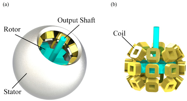
Mechanical structure of RSM: (a) integral structure containing rotor and stator; (b) rotor structure containing coils.

Fig. 2.

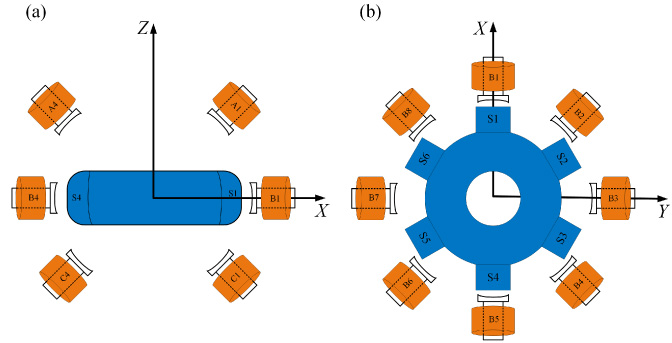
Motion diagram of RSM: (a) diagram of pitching motion; (b) diagram of spinning motion.

Table 1

Main parameters of the RSM

Parameters	Values
Outer diameter of stator	122 mm
Stator magnetic pole width	10 mm
Outer diameter of rotor	73 mm
Rotor pitch	38.75 mm
Coil ampere-turns NI	350

2.2. Mathematical model

The commonly used torque modeling methods for PMSM are the virtual work method, Maxwell tensor method, and Lorentz force method [15–17]. However, there are few studies on the torque modeling of reluctance spherical motors. Because it involves many subject areas such as electrical engineering, control theory, and power electronics, it is very difficult to model the torque using Maxwell tensor method as well as Lorentz force method. Therefore, this paper adopts the virtual work method to model the torque of the RSM. For rotating motors with a core and winding along with a magnetic field as the coupling field, the magnetic energy, magnetic co-energy, and virtual displacement methods can be used to solve for the electromagnetic torque. Let there be n windings connected to the power supply on the stator and rotor of the motor and a rotor that outputs mechanical energy. That is, n electrical ports and 1 mechanical port. Neglecting iron core loss and mechanical loss, then the motor can be seen as an ideal lossless magnetic energy storage system. Taking the flux linkage of n windings 𝛹₁, 𝛹₂, … , 𝛹_n, and the rotor angle θ as independent variables, the magnetic energy of the motor W _m is a function of the flux linkage and the angle of rotation. Let the rotor make a small angular displacement dθ during the time dt, when the change of the flux linkage in each winding is d𝛹₁, d𝛹₂, … , d𝛹_n, respectively. Next, the expression for the electromagnetic torque is derived based on the magnetic and electrical energy as well as the mechanical energy in this system. According to Faraday’s law of electromagnetic induction, when the flux linkage changes, an induced electric potential is generated in the winding, where the electric potential of the kth winding is: $\begin{eqnarray}\displaystyle e_{k}=-\frac{d{\psi}_{k}}{dt}. & & \displaystyle\end{eqnarray}$ (1)

In this case, the kth winding inputs power to the system through the power supply. If the current in winding k is i _k, then after neglecting the losses in the winding resistance R _k, the net power input to the kth winding dW _{e (k)} should be: $\begin{eqnarray}\displaystyle dW_{e(k)}=-e_{k}i_{k}dt=i_{k}d{\psi}_{k}. & & \displaystyle\end{eqnarray}$ (2)

Then the total net electrical energy dW _e input to the coupled field should be: $\begin{eqnarray}\displaystyle dW_{e}=\mathop{\sum }_{1}^{n}dW_{e(k)}=\mathop{\sum }_{1}^{n}i_{k}d{\psi}_{k}. & & \displaystyle\end{eqnarray}$ (3)

Let the electromagnetic torque T _e act on the rotor when the rotor produces a virtual displacement dθ, then the total mechanical energy dW _mech output from the coupling field to the mechanical system is: $\begin{eqnarray}\displaystyle dW_{mech}=T_{e}d{\theta}_{mech}. & & \displaystyle\end{eqnarray}$ (4)

Where θ_mech is the mechanical angle of rotor rotation, θ_mech = θ∕P, and P is the number of pole pairs of the motor. According to the principle of conservation of energy, the net electrical energy input dW _e to the system is equal to the sum of the incremental magnetic energy dW _m and the mechanical energy output dW _mech in dt time, so: $\begin{eqnarray}\displaystyle dW_{e}=dW_{mech}+dW_{m}. & & \displaystyle\end{eqnarray}$ (5)

Substituting Eq. (3) and Eq. (4) into Eq. (5), we get: $\begin{eqnarray}\displaystyle dW_{m}=\mathop{\sum }_{1}^{n}i_{k}d{\psi}_{k}-T_{e}d{\theta}_{mech}. & & \displaystyle\end{eqnarray}$ (6)

And dW _m is a total derivative when expressed as a partial derivative: $\begin{eqnarray}\displaystyle dW_{m}\text{} & =\text{} & \displaystyle \left(\frac{\partial W_{m}}{\partial {\psi}_{1}}d{\psi}_{1}+\frac{\partial W_{m}}{\partial {\psi}_{2}}d{\psi}_{2}+\cdots +\frac{\partial W_{m}}{\partial {\psi}_{n}}d{\psi}_{n}\right)+\frac{\partial W_{m}}{\partial {\theta}}d{\theta}\nonumber\\ \displaystyle \text{} & =\text{} & \displaystyle \mathop{\sum }_{1}^{n}\frac{\partial W_{m}}{\partial {\psi}_{k}}d{\psi}_{k}+p\frac{\partial W_{m}}{\partial {\theta}}d{\theta}_{mech}.\end{eqnarray}$ (7)

Comparing Eq. (6) with Eq. (7), the expression for the electromagnetic torque T _e is: $\begin{eqnarray}\displaystyle T_{e}=-p\frac{\partial W_{m}}{\partial {\theta}}=-\frac{\partial W_{m}}{\partial {\theta}_{mech}}. & & \displaystyle\end{eqnarray}$ (8)

The sum of magnetic co-energy $W_{m}^{\prime }$ and magnetic energy W _m is i𝛹, so the magnetic co-energy $W_{m}^{\prime }$ is as shown in Eq. (9): $\begin{eqnarray}\displaystyle W_{m}^{\prime }(i_{1},i_{2},\ldots ,i_{n},{\theta})=\mathop{\sum }_{1}^{n}i_{k}{\psi}_{k}-W_{m}({\psi}_{1},{\psi}_{2},\ldots ,{\psi}_{n},{\theta}). & & \displaystyle\end{eqnarray}$ (9)

From Eq. (9), when the virtual displacement angle is dθ the increment of magnetic co-energy $dW_{m}^{\prime }$ is: $\begin{eqnarray}\displaystyle dW_{m}^{\prime }(i_{1},i_{2},\ldots ,i_{n},{\theta})\text{} & =\text{} & \displaystyle \mathop{\sum }_{1}^{n}d(i_{k}{\psi}_{k})-dW_{m}({\psi}_{1},{\psi}_{2},\ldots ,{\psi}_{n},{\theta})\nonumber\\ \displaystyle \text{} & =\text{} & \displaystyle \mathop{\sum }_{1}^{n}i_{k}d{\psi}_{k}+\mathop{\sum }_{1}^{n}{\psi}_{k}di_{k}-dW_{m}({\psi}_{1},{\psi}_{2},\ldots ,{\psi}_{n},{\theta}).\end{eqnarray}$ (10)

Substituting Eq. (6) into Eq. (10), we get: $\begin{eqnarray}\displaystyle dW_{m}^{\prime }=\mathop{\sum }_{1}^{n}{\psi}_{k}di_{k}+T_{e}d{\theta}_{mech}. & & \displaystyle\end{eqnarray}$ (11)

When $dW_{m}^{\prime }$ is expressed as a total derivative, we have: $\begin{eqnarray}\displaystyle dW_{m}^{\prime }\text{} & =\text{} & \displaystyle \left(\frac{\partial W_{m}^{\prime }}{\partial i_{1}}di_{1}+\frac{\partial W_{m}^{\prime }}{\partial i_{2}}di_{2}+\cdots +\frac{\partial W_{m}^{\prime }}{\partial i_{n}}di_{n}\right)+\frac{\partial W_{m}}{\partial {\theta}}d{\theta}\nonumber\\ \displaystyle \text{} & =\text{} & \displaystyle \mathop{\sum }_{1}^{n}\frac{\partial W_{m}^{\prime }}{\partial i_{k}}di_{k}+\frac{\partial W_{m}^{\prime }}{\partial {\theta}}d{\theta}.\end{eqnarray}$ (12)

Comparing Eq. (12) with Eq. (11), we get: $\begin{eqnarray}\displaystyle T_{e}=p\frac{\partial W_{m}^{\prime }(i_{1},i_{2},\ldots ,i_{n},{\theta})}{\partial {\theta}}=\frac{\partial W_{m}^{\prime }(i_{1},i_{2},\ldots ,i_{n},{\theta})}{\partial {\theta}_{mech}}. & & \displaystyle\end{eqnarray}$ (13)

Where the magnetic co-energy $W_{m}^{\prime }$ is the integral of 𝛹 over di while holding θ constant: $\begin{eqnarray}\displaystyle W_{m}^{\prime }\text{} & =\text{} & \displaystyle \int _{0}^{i_{1}}{\Psi}_{1}(i_{1}^{\prime },0,\ldots ,0,{\theta})di_{_{1}}^{\prime }+\int _{0}^{i_{2}}{\Psi}_{2}(i_{1},i_{2}^{\prime },0,\ldots ,0,{\theta})di_{_{2}}^{\prime }\nonumber\\ \displaystyle & \text{} & \displaystyle \text{}\quad +\cdots +\int _{0}^{i_{n}}{\Psi}_{n}(i_{1},i_{2},\ldots ,i_{n}^{\prime },{\theta})di_{n}^{\prime }.\end{eqnarray}$ (14)

Equation (13) shows that under the nonlinear magnetic circuit, the differential treatment of the magnetic co-energy gives the value of the torque of the reluctance spherical motor. When the magnetic circuit is linear and has n windings, the relationship between the flux linkage and the current is: $\begin{eqnarray}\displaystyle \left\{\begin{array}{@{}l@{}}{\Psi}_{1}=L_{11}({\theta})i_{1}+L_{12}({\theta})i_{2}+\cdots +L_{1n}({\theta})i_{n}\\ {\Psi}_{2}=L_{21}({\theta})i_{1}+L_{22}({\theta})i_{2}+\cdots +L_{2n}({\theta})i_{n}\\ \cdots \cdots \cdots \cdots \cdots \cdots \cdots \cdots \cdots \cdots \cdots \cdots \cdots \cdots \cdots \\ \cdots \cdots \cdots \cdots \cdots \cdots \cdots \cdots \cdots \cdots \cdots \cdots \cdots \cdots \cdots \\ {\Psi}_{n}=L_{n1}({\theta})i_{1}+L_{n2}({\theta})i_{2}+\cdots +L_{nn}({\theta})i_{n}.\end{array}\right. & & \displaystyle\end{eqnarray}$ (15)

Where L ₁₁, L ₂₂, …, L _nn are the self inductance of the winding, L ₂₁, L ₃₁, …, L _{n, n−1} are the mutual inductance of the winding. Substituting Eq. (15) into Eq. (14): $\begin{eqnarray}\displaystyle W_{m}^{\prime }\text{} & =\text{} & \displaystyle \int _{0}^{i_{1}}[L_{11}({\theta})i_{1}^{\prime }+L_{12}({\theta})i_{2}+\cdots +L_{1n}({\theta})i_{n}]_{i_{2},\ldots i_{n}=0}di_{_{1}}^{\prime }\nonumber\\ \displaystyle \text{} & \text{} & \displaystyle +\int _{0}^{i_{2}}[L_{21}({\theta})i_{1}^{\prime }+L_{22}({\theta})i_{2}+\cdots +L_{2n}({\theta})i_{n}]_{i_{3},\cdots i_{n}=0}di_{_{2}}^{\prime }\nonumber\\ \displaystyle \text{} & \text{} & \displaystyle +\cdots +\int _{0}^{i_{n}}[L_{n1}({\theta})i_{1}^{\prime }+L_{n2}({\theta})i_{2}+\cdots +L_{nn}({\theta})i_{n}]di_{n}^{\prime }\nonumber\\ \displaystyle \text{} & =\text{} & \displaystyle \frac{1}{2}L_{11}({\theta}){i_{1}}^{2}+\frac{1}{2}L_{22}({\theta}){i_{2}}^{2}+\cdots \frac{1}{2}L_{nn}({\theta}){i_{n}}^{2}+L_{12}({\theta})i_{1}i_{2}+L_{13}({\theta})i_{1}i_{3}\nonumber\\ \displaystyle \text{} & \text{} & \displaystyle +\cdots +L_{n,n-1}({\theta})i_{n}i_{n-1}.\end{eqnarray}$ (16) The electromagnetic torque T _e is: $\begin{eqnarray}\displaystyle T_{e}\text{} & =\text{} & \displaystyle p\frac{\partial W_{m}^{\prime }}{\partial {\theta}}=p\left[\frac{1}{2}\frac{\partial L_{11}({\theta})}{\partial {\theta}}{i_{1}}^{2}+\frac{1}{2}\frac{\partial L_{22}({\theta})}{\partial {\theta}}{i_{2}}^{2}+\cdots +\frac{1}{2}\frac{\partial L_{nn}({\theta})}{\partial {\theta}}{i_{n}}^{2}\right]\nonumber\\ \displaystyle \text{} & \text{} & \displaystyle +∼p\left[\frac{\partial L_{12}({\theta})}{\partial {\theta}}i_{1}i_{2}+\frac{\partial L_{13}({\theta})}{\partial {\theta}}i_{1}i_{3}+\cdots +\frac{\partial L_{n,n-1}({\theta})}{\partial {\theta}}i_{n}i_{n-1}\right].\end{eqnarray}$ (17)

Equation (17) shows that the torque value of a reluctance spherical motor can be obtained by differentiating the inductance and then projecting it. To calculate the torque in different directions of the RSM, the specific idea is to first obtain the numerical distribution of the motor inductance to form the inductance surface. Secondly, the inductance differentiation along the longitudinal and latitudinal directions is solved for each place on that surface. Finally, it is simply converted to the Cartesian coordinate system.

Fig. 3.

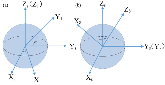
Local coordinate system diagram: (a) diagram of Relative CS₁; (b) diagram of Relative CS₈.

2.3. Global and local coordinate systems

The structure of the RSM has been mentioned before, it has 12 sets of coils in total, so 12 sets of inductors need to be simulated when inductance simulation is performed. Moreover, the electromagnetic torque generated by energized coil in the subsequent simulation is in its corresponding coordinate system. And the torque needs to be converted to the same coordinate system for comparison and verification. Based on the fact that the values of the same torque vector in two different coordinate systems can be converted to each other, the torque under one coordinate system can be converted to the other coordinate system. Based on the above idea, this paper proposes the following solution: simulate the inductance of a pair of coils in the middle layer, calculate the torque value in this coordinate system, and then project it to the rest of the coils in the coordinate system. The coordinate system is specifically set up as follows. The coordinate system of B1 coil is the global coordinate system Globe CS(X _s, Y _s, Z _s) with X _s-axis pointing to the centerline of B1 coil, Y _s-axis pointing to the centerline of B3 coil, and Z _s-axis pointing vertically upward. The coordinate system of B2 coil is the local coordinate system Relative CS₁ (X ₁, Y ₁, Z ₁), with X ₁-axis pointing to the centerline of B2 coil and Y ₁-axis pointing to the centerline of B4 coil, and Z ₁-axis pointing vertically upward. It can be seen that Relative CS₁ is obtained from the Globe CS spin 45°, as shown in Fig. 3(a). The local coordinate system corresponding to the remaining coils in the middle layer can be obtained by rotating the global coordinate system from B2 coil to B8 coil with local coordinate system subscripts from 1 to 7, which will not be repeated here. The local coordinate system of the top and bottom coils corresponding to the stator coils is obtained by pitching on the basis of the global coordinate system spin. As an example, the local coordinate system of Relative CS₈ of A1 coil with the same longitude as B1 coil is obtained by tilting the global coordinate system up 33° around Y _s-axis, as shown in Fig. 3(b). The rest of the upper local coordinate system can be obtained from Relative CS₈ spin, and the subscripts of the local coordinate system from A1 coil to A8 coil are from 8 to 15; similarly, the local coordinate system of the bottom coil is established, and the subscripts of the local coordinate system from C1 coil to C8 coil are from 16 to 23. This completes the establishment of the global and local coordinate systems, and the next step is to project the moments in the global coordinate system to the 23 local coordinate systems. This is done by projecting the moments in the global coordinate system into the local coordinate system according to the angle between the six axes of the global coordinate system and the local coordinate system by using Eq. (18) below. $\begin{eqnarray}\displaystyle \left[\begin{array}{@{}c@{}}TX_{i}\\ TY_{i}\\ TZ_{i}\end{array}\right]=\left[\begin{array}{@{}ccc@{}}COS\angle X_{i}OX_{s} & COS\angle X_{i}OY_{s} & COS\angle X_{i}OZ_{s}\\ COS\angle Y_{i}OX_{s} & COS\angle Y_{i}OY_{s} & COS\angle Y_{i}OZ_{s}\\ COS\angle Z_{i}OX_{s} & COS\angle Z_{i}OY_{s} & COS\angle Z_{i}OZ_{s}\end{array}\right]\left[\begin{array}{@{}c@{}}TX_{s}\\ TY_{s}\\ TZ_{s}\end{array}\right]\quad (i=1,\ldots ,23), & & \displaystyle\end{eqnarray}$ (18) where ∠X _i OX _s is the angle between X _i-axis of the local coordinate system and X _s-axis of the global coordinate system under the condition that the origin of the local and global coordinate systems coincide, and other angles can be similarly understood. This completes the projection of the torque values from the global coordinate system to the local coordinate system.

3. Torque modeling under linear magnetic circuit

3.1. Magnetic circuit distribution of a pair of coils

From Section 2.2, we know that the torque is obtained by differentiating the inductance, and we need to obtain the inductance distribution to solve for the torque value. To obtain the inductance, the spherical motor is simulated in this paper using Ansys finite element simulation software [18–20]. Ansys software can complete two-dimensional and three-dimensional finite element analysis and solution of the motor, and the spherical motor can carry out three-DOF motion, so this paper uses the Maxwell module of Ansys to simulate the spherical motor. According to the specific parameters of the RSM in Table 1, 3D model of the RSM is drawn in Maxwell software. The 3D finite element model of the RSM and its initial position are shown in Fig. 4.

The spatial position of the stator coil is shown in Fig. 5. When unit current is applied to the B1 and B5 coils, the initial position of the rotor is aligned with the B1 coil. The coil inductance is simulated for the rotor from 0° spin to 60° and from 0° pitch to 33°. The inductance variation pattern is shown in Fig. 6. According to Fig. 6, it can be seen that the inductance variation curves of spin and pitch overlap well during the first 30° of rotation, indicating that the contours of inductance in the two-dimensional plane of longitude and latitude are distributed according to a circular law.

Then the next step in solving the flux linkage is to treat only the current value as the radius. The simulation is then repeated with the set of coils (A1 and A5) not located in the middle layer passing a unit current. A comparative of the inductance values for the spin and pitch variations of the mid-level and non-mid-level coils is shown in Fig. 7. It can be seen that the inductance of the coils on the equator and on the non-equator varies in the same pattern, then the same set of data can be used for all coils.

Fig. 4.

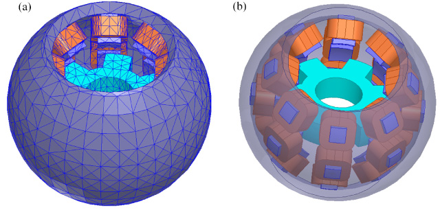
Finite element model: (a) Profile rendering of spherical motor; (b) Simulation starting position.

Fig. 5.

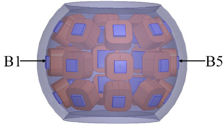
The spatial position of the stator coil.

Fig. 6.

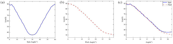
B1 coil magnetic circuit distribution: (a) Spin inductance curve; (b) Pitch inductance curve; and (c) 0–30° inductance curve comparative.

Fig. 7.

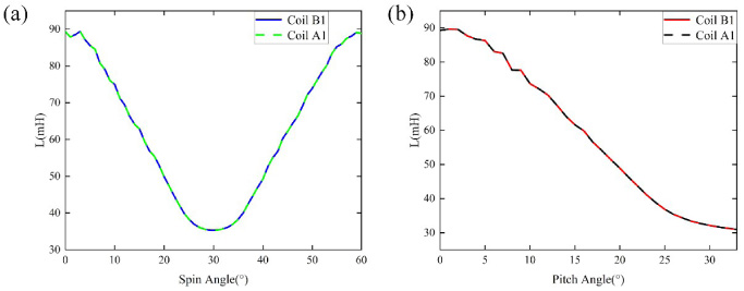
Comparative of the magnetic circuit of B1 coil and A1 coil: (a) Spin inductance comparative; (b) Pitch inductance comparative.

Fig. 8.

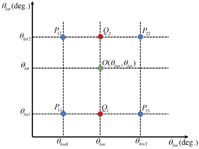
Inductance bilinear interpolation schematic.

Fig. 9.

The inductance surface of B1 coil.

3.2. Interpolation calculation of inductance

After pre-storing an inductance value for a stator coil range in Section 3.1, the inductance value for any point in the coil range can be calculated using bilinear interpolation based on the inductance at a known location point. The horizontal and vertical coordinates in Fig. 8 are the two position variables θ_lon and θ_lat of the inductance function, respectively. 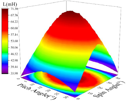To calculate the inductance at any point O, the inductance at the four sampling points P ₁₁, P ₁₂, P ₂₁ and P ₂₂ around the point O should be determined first, and then the inductance at Q ₁ and Q ₂ should be obtained by linear interpolation twice in the θ_lon direction, and then the inductance at point O can be obtained by interpolating the inductance of Q ₁ and Q ₂ once in the θ_lat direction. The interpolation formula is given in the following equation. When the initial position of the rotor is the boundary point of the B1 coil (the position of 22.5° West longitude and 16.5° South latitude), the inductance surface in the B1 coil area obtained by interpolation calculation is shown in Fig. 9. $\begin{eqnarray}\displaystyle L(O)\approx \left(\begin{array}{@{}c@{}}\displaystyle \frac{{\theta}_{lat2}-{\theta}_{lat}}{{\theta}_{lat2}-{\theta}_{lat1}}\left(\frac{{\theta}_{lon2}-{\theta}_{lon}}{{\theta}_{lon2}-{\theta}_{lon1}}L(P_{11})+\frac{{\theta}_{lon}-{\theta}_{lon1}}{{\theta}_{lon2}-{\theta}_{lon1}}L(P_{21})\right)\\[12.0pt] \displaystyle +\frac{{\theta}_{lat}-{\theta}_{lat1}}{{\theta}_{lat2}-{\theta}_{lat1}}\left(\frac{{\theta}_{lon2}-{\theta}_{lon}}{{\theta}_{lon2}-{\theta}_{lon1}}L(P_{12})+\frac{{\theta}_{lon}-{\theta}_{lon1}}{{\theta}_{lon2}-{\theta}_{lon1}}L(P_{22})\right)\end{array}\right). & & \displaystyle\end{eqnarray}$ (19)

3.3. Inductance differentiation and projection calculation

From Section 3.1, we can obtain the inductance surface of B1 coil when unit currents are passed to B1 and B5 coils. After obtaining this inductance surface, we can obtain Eq. ((20)) from Eq. ((17)): $\begin{eqnarray}\displaystyle \left\{\begin{array}{@{}l@{}}\displaystyle T_{lat}=\frac{1}{2}pi^{2}\frac{\partial L_{lat}}{\partial {\theta}_{lat}}\\[12.0pt] \displaystyle T_{lon}=\frac{1}{2}pi^{2}\frac{\partial L_{lon}}{\partial {\theta}_{lon}}\end{array}.\right. & & \displaystyle\end{eqnarray}$ (20)

Where L _lon represents the inductance array when rotor convex pole at different longitudes positions while keeping the same latitude; L _lat represents the inductance array when rotor convex pole at different latitudes positions while keeping the same longitude. This gives the values of the torques in the latitude and longitude directions calculated in the global coordinate system. The differential surfaces in the latitudinal and longitudinal directions are shown in Fig. 10. From the figure, it can be seen that the torque in the latitudinal direction will have burrs in spin 0–8° and in pitch between 28° and 45°, which is caused by the finite element profile not fine enough during the inductor simulation.

Fig. 10.

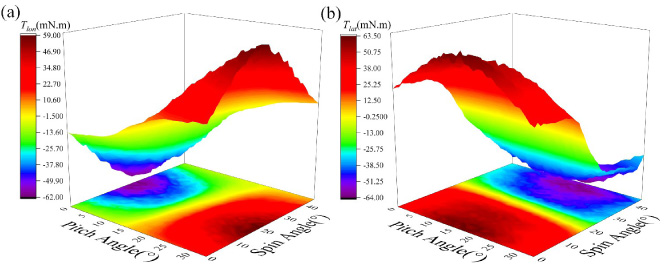
Differential calculation result: (a) Latitude inductance differential; (b) Longitude inductance differential.

In Section 2.3, we have already described how to project the moments in the global coordinate system to the local coordinate system, and now we describe how to convert the moments in the latitude and longitude directions to the global coordinate system. After taking any point P (θ_lat, θ_lon) of the sphere and projecting the latitude and longitude coordinates to the orthogonal coordinates, the projection vector diagram is shown in Fig. 11, and the defined position of the coordinate axes is the same as Fig. 2.

Fig. 11.

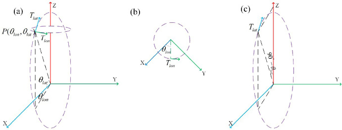
Vector diagram: (a) Overall projection vector diagram; (b) Longitude projection vector diagram; (c) Latitude projection vector diagram.

The formula for converting the latitude and longitude torques to the global coordinate system can be obtained from the figure as $\begin{eqnarray}\displaystyle \left\{\begin{array}{@{}l@{}}TX_{s}=-T_{lon}\sin {\theta}_{lon}-T_{lat}\cos (90^{\circ }-{\theta}_{lat})\cos {\theta}_{lon}\\[6.0pt] TY_{s}=T_{lon}\cos {\theta}_{lon}-T_{lat}\cos (90^{\circ }-{\theta}_{lat})\sin {\theta}_{lon}\\[6.0pt] TZ_{s}=T_{lat}\sin (90^{\circ }-{\theta}_{lat})\end{array}.\right. & & \displaystyle\end{eqnarray}$ (21) Substituting Eq. (20) into Eq. (21) yields: $\begin{eqnarray}\displaystyle \left\{\begin{array}{@{}l@{}}\displaystyle TX_{s}=-\frac{1}{2}pi^{2}\frac{\partial L_{lon}}{\partial {\theta}_{lon}}\sin {\theta}_{lon}-\frac{1}{2}pi^{2}\frac{\partial L_{lat}}{\partial {\theta}_{lat}}\cos (90^{\circ }-{\theta}_{lat})\cos {\theta}_{lon}\\[12.0pt] \displaystyle TY_{s}=\frac{1}{2}pi^{2}\frac{\partial L_{lon}}{\partial {\theta}_{lon}}\cos {\theta}_{lon}-\frac{1}{2}pi^{2}\frac{\partial L_{lat}}{\partial {\theta}_{lat}}\cos (90^{\circ }-{\theta}_{lat})\sin {\theta}_{lon}\\[12.0pt] \displaystyle TZ_{s}=\frac{1}{2}pi^{2}\frac{\partial L_{lat}}{\partial {\theta}_{lat}}\sin (90^{\circ }-{\theta}_{lat})\end{array}.\right. & & \displaystyle\end{eqnarray}$ (22)

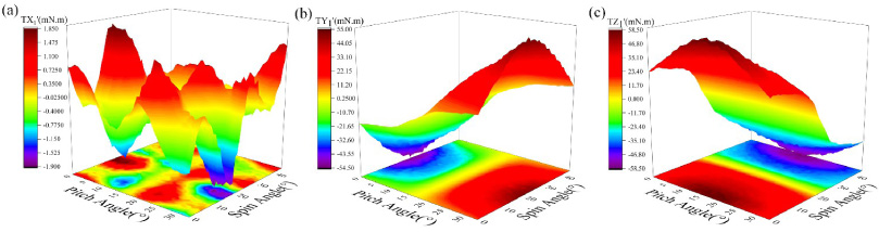
After calculating the inductance differential of B1 coil in longitude and latitude direction and substituting the differentiation result into Eq. (22), the conversion of the two-DOF torque to the global coordinate system is completed. Next, the torque value in the global coordinate system of the B1 coil is projected to the local coordinate system of the B2 coil, and the torque in the local coordinate system is obtained by substituting the three-axis torque in the global coordinate system and the nine projection angles into Eq. (18). The results of parsing calculation are shown in Fig. 12.

Fig. 12.

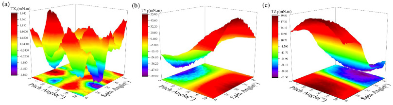
Analytical calculation of three-axis torque diagram: (a) X-axis torque; (b) Y -axis torque; and (c) Z-axis torque.

3.4. Finite element simulation verification

Coils B2 and B6 will be passed with the unit current, rotating a magnetic pole from B2 coil space position of an inflection point that is 22.5° West longitude and 16.5° South latitude. First spin 45° at 1° step to 22.5 °E, then pitch 1° and spin 45° at 1° steps to finally reach the position of 22.5 °E and 16.5 °N. The torque values for this process are simulated, which are shown in Fig. 13.

Fig. 13.

Simulation of three-axis torque diagram: (a) X-axis torque; (b) Y-axis torque; (c) Z-axis torque.

To facilitate the comparative, a local verification is first performed. One boundary line of B2 coil, i.e., the position of 22.5 °W 16.5 °S to the observation line of 22.5 °W 16.5 °N, is taken to compare with the triaxial torques. The comparative results are shown in Fig. 14. From the figure, it can be seen that the torque on the observation line is highly agreement with the finite element results.

Fig. 14.

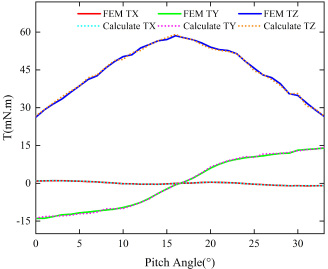
Torque comparative.

Then the global verification is performed, the absolute error value is taken as the result of subtracting the analytical calculation value from the simulation value. The absolute error value is divided by the simulation value to obtain the relative error, torque error percentage is shown in Fig. 15. Among them, the maximum percentage of X-axis torque error is 3.03%; the maximum percentage of Y -axis torque error is 3.32%; the maximum percentage of Z-axis torque error is 3.56%. It can be seen that the relative error of X-axis is smaller than that of Y -axis and Z-axis. The error in both directions is mainly due to the fluctuation of the inductance values from the finite element simulation, which leads to a certain error in the differential calculation. Compared with the finite element method, the down time saved by the virtual work method for calculating torque is shown in Table 2.

Fig. 15.

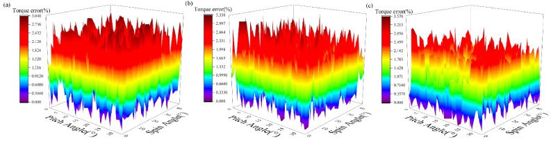
Torque error percentage diagram: (a) X-axis torque error percentage; (b) Y-axis torque error percentage; and (c) Z-axis torque error percentage.

Table 2

Comparative of computing time

Modeling method	FEM	Virtual work method
Time	6.3 h	1.3 s

4. Torque modeling under nonlinear magnetic circuit

4.1. Calculation of magnetic co-energy

Using the inductance value obtained by linear interpolation in Section 3.2, the distribution of flux linkage curves for the rotor passing through different spatial positions of the B1 coil is obtained by substituting into the equation 𝛹 = IL. Since the inductance curves of the first 30° of spin and pitch during rotation are highly overlapping, only the flux linkage in the spin direction needs to be analyzed. It can be seen from Fig. 6(a) that the inductance is symmetric about 30° during the spinning process, so it is enough to analyze the 0–30° flux linkage curve. The spin angle of the rotor is set to the variable euler, and the distribution of flux linkage curves with spin 0–30° is solved as shown in the Fig. 16 below.

Fig. 16.

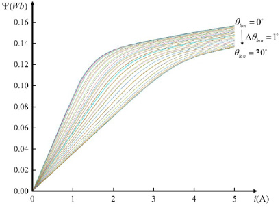
Flux linkage curve distribution.

The bending of the inductance curve is most obvious at 0° as seen in Fig. 16, and the magnetic circuit starts to saturate when i =1.6A, and the flux linkage becomes nonlinear with the current. Calculate the magnetic co-energy with spin 0° as an example: Since the maximum input current of the control board is 3A, calculate the magnetic co-energy at i =3A.

Fig. 17.

Magnetization curve at θ = 0°.

Fig. 18.

Magnetic co-energy curve.

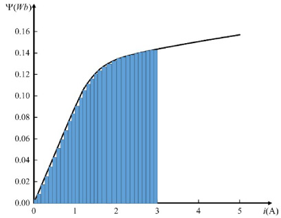
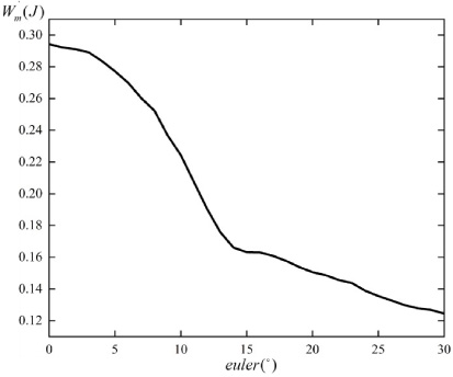
When the current is constant, the magnetic co-energy is equal to the integral of the flux linkage 𝛹 over the current i. As can be seen from the Fig. 17, the current is divided linearly from 0–3A in steps of 0.1A, and the integration formula is used to calculate within each segment, and the integration results of each segment are summed up to be the final integration result. So the magnetic function at 0° can be calculated according to Eq. (23), and the rest of the angles are processed according to this procedure. The magnetic co-energy at different angles is shown in the Fig. 18. $\begin{eqnarray}\displaystyle W_{{\theta}}^{\prime }=\int _{0}^{3}{\psi}di\approx \mathop{\sum }_{i=0}^{30}(I_{i+1}-I_{i}){\psi}\left(\frac{I_{i}+I_{i+1}}{2}\right). & & \displaystyle\end{eqnarray}$ (23)

4.2. Simulation verification

When the rotor passes through the stator coil in different directions, the change of the magnetic co-energy is different. Where $W_{{\theta}lon}^{\prime }$ represents the magnetic co-energy array when rotor convex pole at different longitudes positions while keeping the same latitude; $W_{{\theta}lat}^{\prime }$ represents the magnetic co-energy array when rotor convex pole at different latitudes positions while keeping the same longitude. After obtaining the magnetic co-energy surface, the differential processing and projection operations in the longitudinal and latitudinal directions are performed respectively, and the results of the torque in the three axes can be calculated from Eq. ((24)). The differentiation and projection operations are similar to those in Section 3.3 and will not be repeated here. $\begin{eqnarray}\displaystyle \left\{\begin{array}{@{}l@{}}\displaystyle TX=-p\frac{\partial {W^{\prime }}_{{\theta}_{lon}}}{\partial {\theta}_{lon}}\sin {\theta}_{lon}-p\frac{\partial {W^{\prime }}_{{\theta}_{lat}}}{\partial {\theta}_{lat}}\cos (90^{\circ }-{\theta}_{lat})\cos {\theta}_{lon}\\[12.0pt] \displaystyle TY=p\frac{\partial {W^{\prime }}_{{\theta}_{lon}}}{\partial {\theta}_{lon}}\cos {\theta}_{lon}-p\frac{\partial {W^{\prime }}_{{\theta}_{lat}}}{\partial {\theta}_{lat}}\cos (90^{\circ }-{\theta}_{lat})\sin {\theta}_{lon}\\[12.0pt] \displaystyle TZ=p\frac{\partial {W^{\prime }}_{{\theta}_{lat}}}{\partial {\theta}_{lat}}\sin (90^{\circ }-{\theta}_{lat})\end{array}.\right. & & \displaystyle\end{eqnarray}$ (24)

The B1 coil through 3A current, the rotor a magnetic pole pitch through the B1 coil of a boundary line that is 67.5° West longitude 16.5° South latitude position to 22.5° West longitude 16.5° South latitude this observation line to compare the three-axis torque. The comparative results are shown in the Fig. 19, from the figure can be seen on the observation line torque and finite element results highly overlap.

Fig. 19.

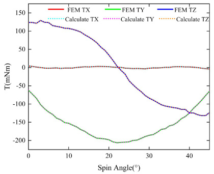
Torque comparative.

5. Experiments and analysis

5.1. Introduction to the experimental platform

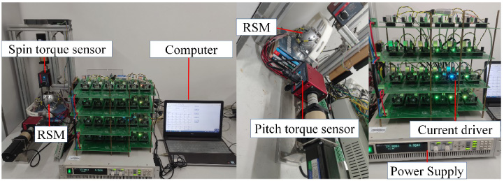
In order to verify the accuracy of the modeling method, an experiment platform consisting of the computer, power supply, motor prototype, current driver, dynamic torque sensor, and torque detection bench was built for the experiment. The device diagram of the experiment is shown in Fig. 20. The current driver is composed of 24 independent constant current drive units, and each unit has a separate ARM controller, the model of ARM processor is STM32F407VGT6. The control signal sent by the computer is transmitted to each drive module through the signal line, which can supply current to 24 stator coils. The power supply supplies power to the current driver. The dynamic torque sensor can record the torque value during the motor output shaft movement, the model of sensor is DYN-200 can detect torque in the range of 0–5 N⋅m. The torque detection bench is used to connect the rotor output shaft and the torque sensor.

Since the motor structure is symmetrical in X-axis and Y-axis directions, it is sufficient to measure the torque in one direction. The output shaft of the spherical motor rotor is connected horizontally through the rotating bracket, and the torque sensor and the rotating shaft of the rotating bracket are coaxial and extend through the rotor sphere center. When the rotor ball is in the initial position (rotor one pole is directly opposite to B1 and B5 stator coils) and 1A current is applied to the upper A1 and lower C5 coils, the rotor output shaft will carry the rotation axis in a pitching motion, and the torque data during the pitching process will be recorded. In the vertical direction, the torque sensor is connected to the output shaft by coupling, with the rotor ball still in the initial position. When 1A current is passed to the middle B2 and B6 coils, the rotor output shaft drives the rotating shaft of the torque sensor to make a spin motion and records the torque data during the spin.

Fig. 20.

Experimental device diagram.

5.2. Experiment results and analysis

The values displayed by the torque sensor during the motion are extracted and compared with the torque calculated by the AM. From the torque comparative in Fig. 21, it can be seen that the experimental torque values are slightly lower than the analytic calculation. The relative error of the experimental torque is shown in Fig. 22, the maximum error percentage of spin torque is 4.7%, and the maximum error percentage of pitch torque is 4.53%. The main causes of experimental errors are the following: (a) Position control accuracy causes deviation of actual measurement points of the calculated inductance; (b) There is an error in the torque sensor during the spin (pitch) motion of the rotor; (c) Since the spherical motor contains a support structure, the friction generated during the rotor movement has some influence on the torque measurement; and (d) The effect of gravity on the testing mechanism can cause bias in the results of torque measurement.

Fig. 21.

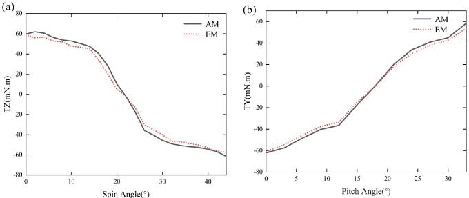
Comparative of torque results: (a) Spin comparative; (b) Pitch comparative.

Fig. 22.

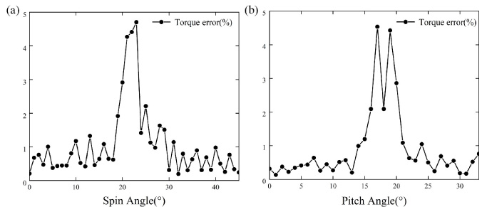
Relative error diagram of experimental torque: (a) Relative error of spin motion; (b) Relative error of pitch motion.

6. Conclusion

In this paper, a modeling and analysis method of RSM is carried out. The main tasks are fulfilled as follow:

Local and global coordinate systems are established, based on the fact that torque value in these two orthogonal coordinate systems can be converted to each other by projection.

RSM inductance model is established by combining the FEM results with linear interpolation.

A torque model is established based on virtual work method. The feasibility and effectiveness of this method are verified by experiment and simulation comparisons.

The model building method in this paper greatly reduces the time while ensuring the accuracy of the model, and solves the problem of long time consuming with finite element calculation. The torque in the global coordinate system established can be extended to each local coordinate system, which greatly reduces the simulation workload. Finally, the torque model obtained is also instructive for the energization strategy and real-time control of RSM.

Footnotes

Acknowledgements

This work is supported by the Nature Science Research Project of Anhui province (1908085QE236).

References

Lee

K.M.

and Kwan

C.K.

, Design concept development of a spherical stepper for robotic applications, IEEE Transactions on Robotics and Automation 7(1) (1991), 175–181.

Lee

K.M.

Sosseh

R.A.

and Wei

Z.Y.

, Effects of the torque model on the control of a VR spherical motor, Control Engineering Practice 12(11) (2004), 1437–1449.

Xia

Song

and Shi

, Research on torque calculation method of permanent-magnet spherical motor based on the finite-element method, IEEE Transactions on Magnetics 45(4) (2009), 2015–2022.

Kahlen

Voss

Priebe

and De Doncker

R.W.

, Torque control of a spherical machine with variable pole pitch, IEEE Transactions on Power Electronics 19(6) (2004), 1628–1634.

Son

and Lee

K.M.

, Distributed multipole models for design and control of PM actuators and sensors, IEEE/ASME Transactions on Mechatronics 13(2) (2008), 228–238.

Lee

K.M.

and Son

, Distributed multipole model for design of permanent-magnet-based actuators, IEEE Transactions on Magnetics 43(10) (2007), 3904–3913.

and Li

, Magnetic field analysis of 3-DOF permanent magnetic spherical motor using magnetic equivalent circuit method, IEEE Transactions on Magnetics 47(8) (2011), 2127–2133.

Rossini

Chetelat

Onillon

and Perriard

, Force and torque analytical models of a reaction sphere actuator based on spherical harmonic rotation and decomposition, IEEE/ASME Transactions on Mechatronics 18(3) (2013), 1006–1018.

Zhou

Wang

and Qiao

, Torque modelling and validation for a spherical motor with stepped permanent magnets, Journal of Electrical Engineering & Technology 15(6) (2020), 2661–2673.

10.

Wang

Zheng

Zhou

Wang

and He

, Research on torque analytical model of permanent-magnet spherical motor based on torque map by Lorentz force method, International Journal of Applied Electromagnetics and Mechanics 65(4) (2021), 735–752.

11.

Tao

Wang

Zhou

and Qiao

, Nonlinear modeling analysis of a reluctance spherical motor based on torque-angle characteristics, International Journal of Applied Electromagnetics and Mechanics 62(3) (2020), 577–593.

12.

Lee

Kim

Bake

Rhyu

and Kwon

, Newly structured double excited two-degree-of-freedom motor for security camera, IEEE Transactions on Magnetics 44(11) (2008), 4041–4044.

13.

Kim

Lee

and Kwon

, Experiment and torque modeling of double-excited, two-degree-of-freedom motor based on magnetic equivalent circuit analysis, Journal of Electrical Engineering & Technology 8(1) (2013), 130–136.

14.

Wang

Qiao

Zhou

and He

, Structural design of salient pole type reluctance spherical motor, Electric Machines and Control 25(1) (2021), 90–102.

15.

Zhao

and Cui

, Torque calculation of permanent magnet spherical motor based on virtual work method, IEEE Transactions on Industrial Electronics 67(9) (2020), 7736–7745.

16.

Lee

K.M.

Bai

and Lim

, Dipole models for forward/inverse torque computation of a spherical motor, IEEE-ASME Transactions on Mechatronics 14(1) (2009), 46–54.

17.

Zhou

Wang

and He

, Torque calculation of permanent-magnet spherical motor based on permanent-magnet surface current and lorentz force, IEEE Transactions on Magnetics 56(5) (2020), 8200209.

18.

Wen

Wang

Guo

and Cao

, Modeling and analysis of permanent magnet spherical motors by a multi-task Gaussian process method and finite element method for output torque, IEEE Transactions on Industrial Electronics 68(9) (2020), 8540–8549.

19.

Wen

Wang

Tang

Liu

and Li

, Investigation on the measurement method for output torque of a spherical motor, Applied Sciences-Basel 10(7) (2020)2510.

20.

Hasanzadeh

Rezaei

and Qiyassi

, Analysis and optimization of permanent magnet dimensions in electrodynamic suspension systems, Journal of Electrical Engineering & Technology 13(1) (2018), 307–314.