A calibration method of ground-airborne frequency domain electromagnetic receving system based on magnetic source excitation

Abstract

In the ground-airborne frequency domain electromagnetic detection, the receving system converts the magnetic field signal into an electrical signal representing the magnetic field signal. In order to accurately obtain the relationship between the magnetic field signal and the electrical signal, it is necessary to avoid the influence of environment and other factors on the system accuracy through on-site calibration. This requires high calibration accuracy, simple operation, portable equipment and strong adaptability to the environment. However, the existing calibration methods put forward higher requirements for instruments and environment. For example, the calibration of uniform magnetic field generated by Helmholtz coil needs to shield external magnetic field interference. In this paper, an overall calibration method of measurement system based on magnetic source excitation is proposed to meet the requirements of electromagnetic field accurate measurement in ground-airborne frequency domain. Firstly, based on the electromagnetic measurement method in ground-airborne frequency domain, the overall calibration method and principle of the detection system are introduced. Then, based on the computable standard magnetic field generated by the magnetic source transmitting coil, determine the measured voltage obtained by the receiving system, get the calibration coefficient of the receiving system. At last,the source of standard uncertainty related to calibration is analyzed, and the uncertainty is evaluated. In addition, the method is verified by comparing the calibration results with those obtained by Braunbeck coil calibration.

Keywords

Ground-air frequency domain electromagnetic detection air-core sensor (ACS)magnetic source excitation calibration

1. Introduction

Ground-airborne frequency domain electromagnetic method uses the ground high-power artificial electromagnetic source as the excitation field source, and collects the magnetic field signals in the air to realize the rapid exploration of the electrical structure of the earth. The system works as shown in Fig. 1. This method combines the dual advantages of high-power emission of ground electromagnetic method and rapid non-contact acquisition of airborne electromagnetic method, and has the potential of rapid detection of areas with complex surface conditions in a large depth range. Essentially, the ground transmitting system injects alternating current with known frequency into the earth through transmitting cables and electrodes, and forms an electromagnetic field with certain intensity in space. The electromagnetic field is coupled with the underground target body, which generates electromagnetic anomalies. The air receiving system can determine the position, buried depth, size and other information of the abnormal body by identifying the anomalies at different frequencies. Ground-airborne frequency domain electromagnetic detection method is widely used in mineral exploration, geological survey, groundwater survey and other fields, especially in the rapid detection of deep structures in complex terrain areas [1–3].

Fig. 1.

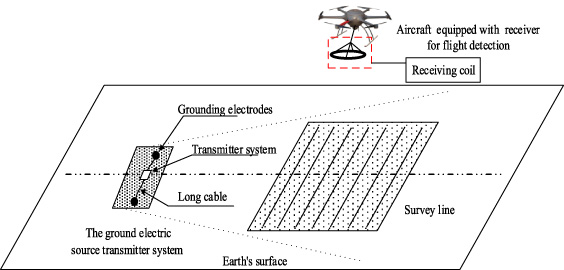
A horizontal long wire source is used as the excitation source of the space magnetic field to generate a primary field, which propagates in the medium. When the primary magnetic field contacts the earth to be detected, induced eddy current and secondary magnetic field are generated. The sensor and receiving system are used to receive these signals; Usually, the sending and receiving distance is several kilometers.

The receiving system consists of an ACS and a receiver. As the first receiving part of the system, the ACS collects signals in the air and converts the dynamic magnetic field into induced voltage, which is an important time-varying magnetic field measuring tool. Before processing the electrical signal representing the magnetic field signal, it must be reduced to the real magnetic field signal, so it is necessary to obtain the influence curve of the magnetic sensor on the magnetic field signal in amplitude and phase, that is, the curve representing the relationship between the magnetic field and the electrical signal, which is called the sensitivity curve. In ground-airborne frequency domain electromagnetic detection, it is necessary to establish the relationship between frequency domain induced voltage and magnetic induction intensity through sensitivity coefficient. And the receiver realizes analog-to-digital conversion, reduces noise and stores data. Whether the sensitivity is accurate or not directly affects the measurement results. However, during the long-term use of the system, the parameters will be disturbed due to environmental changes, bumping during transportation and other reasons, which will lead to the change of sensor sensitivity, which is inconsistent with the theoretical calculation value. Rreference [4] points out that the change of coil turns will have a dramatic impact on the results of transient electromagnetic detection. Reference [5] pointed out that in the application fields of tunnel detection and mineral exploration, the inductance parameters of air-core coil devices will obviously be affected by the relative permeability of environmental media. The A/D conversion circuit of the preamplifier circuit and the data processing circuit in the receiver will also have zero offset during using.

These factors lead to the deviation between the actual parameters of the ACS, preamplifier circuit and receiver in the system and the theoretical values, Thereby causing the error between the measured voltage and the actual voltage. And it is difficult to simulate the influence of field environmental changes on the sensitivity in the laboratory environment. In order to ensure that the system can still guarantee the reliability of the measurement results in the presence of factors affecting the system reliability, it is necessary to calibrate the whole electromagnetic ground-penetrating measurement system in the ground-airborne frequency domain on site. Calibrate an appropriate sensitivity coefficient for the system to obtain more accurate induced voltage parameters, which is very important for the system to achieve accurate measurement. In the literature, according to different research fields, various calibration techniques have been applied. There are two main calibration methods, namely time domain calibration and frequency domain calibration. Time-domain calibration method mainly realizes error correction by eliminating the transition process, for example, reference [6] constructs a relationship between the calibration file and the zero-input response of the ACS and shorten the time required for calibration. Reference [7–9] put forward a ground transient electromagnetic calibration system based on conductive ring, through which the analysis of the transition process is completed. However, due to the unexpected correspondence, the method of converting the measured value into the real induced voltage through the functional relationship is not accurate, and the adaptability to high conductivity soil is poor. Among many calibration methods in frequency domain. Reference [10] obtains the transfer function of the coil by fitting the frequency response of the coil, and eliminates the transition process, thus achieving better performance in shallow detection, but the calibration method of generating uniform magnetic field can’t be applied to the calibration of large coils and can’t meet the needs of ground-to-air measurement. Reference [11] applies the sweep signal to the coil by resonance method to obtain its resonance frequency, and obtains the parameters of coil by calculation. To sum up, these frequency domain calibration methods have higher requirements for calibration environment, calibration magnetic field and test equipment accuracy. There are still some other methods for calibration, including reference [10] calibrating the sensor by fitting the frequency responses at different frequencies to obtain calibration files; The empirical formula proposed in reference [12] and the finite element simulation proposed in reference [5]. However, because the error between the simulation coil model and the actual coil can’t be ignored, the calculation accuracy of these methods may have problems. Therefore, in order to ensure the reliability of the sensitivity coefficient and the accuracy of the measurement results, the sensitivity coefficient which is more accurate than the theoretical calculation value can be obtained through on-site calibration.

Standard field method, that is, calibration by using the calculated field strength. Different authors have proposed different standard field methods, such as long cylindrical winding, current loop in two orthogonal planes, Helmholtz coil and Maxwell coil, to produce uniform standard magnetic field [10,13]. As the ground-airborne electromagnetic detection method adopts the separation of transceiver equipment, the distance between transceiver and transceiver is usually 5-15 km, so as to avoid primary magnetic field saturation and ensure that the area to be detected is approximately plane wave. The size of the ACS is one of the determining factors of the maximum transmit-send distance. In addition, since the ground-to-air electromagnetic detection method is applied in a variety of complex environments, the future development will be widely used in helicopters carrying large coils and corresponding receivers as signal acquisition equipment, and the radius of the sensor may be 5 m or above. It is difficult to calibrate the signal acquisition instrument. Usually, the volume ratio of the device that produces a highly uniform magnetic field to the volume ratio of the generated field is 10:1 or higher. Therefore, the traditional standard field calibration method can not meet the requirements of ground-airborne electromagnetic detection system.

To sum up, in order to realize the field calibration of large ACS, this paper proposes the calculation magnetic field excited by magnetic source as the calibration system to calibrate the receiving system. It achieves accurate measurement by ground-airborne electromagnetic detection method, and solves the problems in the calibration field of large coils, such as high requirements for calibration environment, complex magnetic field generating equipment and complex operation by traditional methods. The method proposed in this paper has strong exploitativeness and portable equipment to meet the requirements of field calibration. In this paper, the main design of calibration system is introduced comprehensively, the source of error is analyzed deeply, and the uncertainty of calibration is reduced by different methods. Finally, the reliability of the proposed method is verified by comparative experiments.

2. Analysis of magnetic field generated by standard magnetic source excitation

2.1. Layered earth simulation model

When the magnetic source is placed parallel to the earth, ACS is in the total field of the primary field and the secondary field reflected by the earth. In order to ensure that the calculated induced voltage value accords with the reality, it is necessary to determine the geodetic model according to the use environment to facilitate the simulation calculation, and consider the index requirements of simulation parameters according to the actual situation. Usually, in the absence of special magnetic anomalies, the earth is considered as a uniform layered model.

As shown in Fig. 2, a two-layer geodetic model is established, in which the conductivity of air σ₀ is 0, and the first and second layers are uniform strata with a thickness of 500 m and a conductivity of σ₁, σ₂ = 0.01 S/m, so as to simulate the uniform half-space underground structure. In order to ensure that the calculated induced voltage value accords with the reality, it is necessary to determine the geodetic model according to the use environment to facilitate the simulation calculation, and consider the index requirements of simulation parameters according to the actual situation.

Fig. 2.

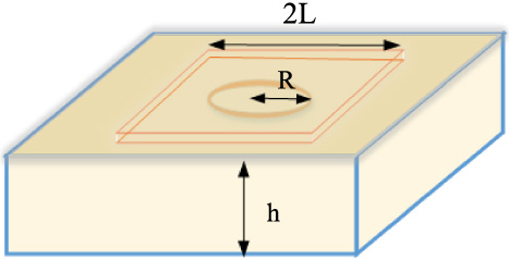
Uniform earth model.

Fig. 3.

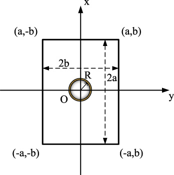
Relative position diagram of rectangular wireframe and ACS.

2.2. Calculation of magnetic field generated by standard magnetic source

The rectangular coordinate system is adopted, the origin is in the center of the rectangular ring, and the Z axis is downward. Figure 3 shows the coordinate system including rectangular loop and dipole source projection and the geometry of the earth surface. The length of the ring is 2a parallel to the x axis and 2b parallel to the y axis. Because of the symmetry of the circle, the electric field of dipole source has only one tangential component E. Place the center of the hollow coil sensor and the center of the transmitting coil at the origin of the coordinate system, with the X axis parallel to the width of the rectangular ring and the Y axis parallel to the length of the rectangular ring. (x, y) is any point on the plane, then the magnetic field intensity of any point in the ACS can be calculated according to Biot-Savart law:

The rectangular transmitting coil is placed on the layered uniform earth, and the magnetic field generated by 2L long wire source is placed in the direction of origin x: $\begin{eqnarray}\displaystyle H_{Z}\text{} & =\text{} & \displaystyle \frac{I}{4{\pi}}\int _{-L}^{L}\frac{y}{R}dx^{\prime }\int _{0}^{\infty }(1+r_{TE})e^{{\mu}_{0}z}\frac{{\lambda}^{2}}{{\mu}_{0}}J_{1}({\lambda}R)d{\lambda}\end{eqnarray}$ (2.1) $\begin{eqnarray}\displaystyle u_{0}\text{} & =\text{} & \displaystyle ({\lambda}^{2}-k_{0}^{2})^{1/2}\end{eqnarray}$ (2.2) $\begin{eqnarray}\displaystyle k_{0}^{2}\text{} & =\text{} & \displaystyle {\mu}_{0}{\varepsilon}_{0}{\omega}^{2}-i{\mu}_{0}{\sigma}_{0}{\omega}\end{eqnarray}$ (2.3) $\begin{eqnarray}\displaystyle u_{n}\text{} & =\text{} & \displaystyle ({\lambda}^{2}-k_{n}^{2})^{1/2}\end{eqnarray}$ (2.4) $\begin{eqnarray}\displaystyle k_{n}^{2}\text{} & =\text{} & \displaystyle {\mu}_{n}{\varepsilon}_{n}{\omega}^{2}-i{\mu}_{n}{\sigma}_{n}{\omega}.\end{eqnarray}$ (2.5)

In which, μ₀, ϵ₀, σ₀ are the permeability, dielectric constant and conductivity in the air layer respectively, and μ_n, ϵ_n, σ_n are the permeability, dielectric constant and conductivity of the nth earth layer respectively; j ₁ is one kind of first-order Bessel function. 𝜆 is Hankel integral variable, r _TE is the reflection coefficient related to the underground electrical structure, I is the excitation current in the transmitting coil, and k is the electromagnetic wave propagation constant.

Then the total magnetic field generated by the Magnetic excitation calibration system is: $\begin{eqnarray}\displaystyle H_{Z}=\frac{I}{4{\pi}}(A_{1}+B_{1}+C_{1}+D_{1}) & & \displaystyle\end{eqnarray}$ (2.6)

Analyze the influence of uniform earth resistivity on magnetic flux, where A ₁, B ₁, C ₁, D ₁ are the integrals of the four sides of the corresponding rectangle. $\begin{eqnarray}\displaystyle A_{1}\text{} & =\text{} & \displaystyle -(b-y)\int _{-a}^{a}\frac{1}{R_{A}}dx^{\prime }\int _{0}^{\infty }(1+r_{TE})e^{u_{0}z}\frac{{\lambda}^{2}}{u_{0}}J_{1}({\lambda}R_{A})d{\lambda}\end{eqnarray}$ (2.7) $\begin{eqnarray}\displaystyle R_{A}\text{} & =\text{} & \displaystyle [(x^{\prime }-x)^{2}+(b-y)^{2}]^{1/2}\end{eqnarray}$ (2.8) $\begin{eqnarray}\displaystyle B_{1}\text{} & =\text{} & \displaystyle -(a-x)\int _{-b}^{b}\frac{1}{R_{B}}dy^{\prime }\int _{0}^{\infty }(1+r_{TE})e^{u_{0}z}\frac{{\lambda}^{2}}{u_{0}}J_{1}({\lambda}R_{B})d{\lambda}\end{eqnarray}$ (2.9) $\begin{eqnarray}\displaystyle R_{B}\text{} & =\text{} & \displaystyle [(a-x)^{2}+(y^{\prime }-y)^{2}]^{1/2}\end{eqnarray}$ (2.10) $\begin{eqnarray}\displaystyle C_{1}\text{} & =\text{} & \displaystyle -(b+y)\int _{-a}^{a}\frac{1}{R_{C}}dx^{\prime }\int _{0}^{\infty }(1+r_{TE})e^{u_{0}z}\frac{{\lambda}^{2}}{u_{0}}J_{1}({\lambda}R_{C})d{\lambda}\end{eqnarray}$ (2.11) $\begin{eqnarray}\displaystyle R_{C}\text{} & =\text{} & \displaystyle [(x^{\prime }-x)^{2}+(b+y)^{2}]^{1/2}\end{eqnarray}$ (2.12) $\begin{eqnarray}\displaystyle D_{1}\text{} & =\text{} & \displaystyle -(a+x)\int _{-b}^{b}\frac{1}{R_{D}}dy^{\prime }\int _{0}^{\infty }(1+r_{TE})e^{u_{0}z}\frac{{\lambda}^{2}}{u_{0}}J_{1}({\lambda}R_{D})d{\lambda}\end{eqnarray}$ (2.13) $\begin{eqnarray}\displaystyle R_{D}\text{} & =\text{} & \displaystyle [(a+x)^{2}+(y^{\prime }-y)^{2}]^{1/2}.\end{eqnarray}$ (2.14)

Where 2a and 2b are the width and length of the rectangular transmitting coil, (x, y) is the coordinates of any point in the ACS, ω = 2πf and f is the transmitting frequency.

The magnetic induction intensity under different conditions is simulated, and the magnetic field obtained is the sum of the initial magnetic field and the reflected magnetic field. The effects of different frequency point responses on magnetic field used in practice are analyzed. Figure 4 Compared and simulated the influence of earth resistivity error on the calibration field, it can be seen that the reflected magnetic field under the strong initial magnetic field has a very weak influence on the calculation results, and quantitatively analyzed the influence of earth resistivity error on the calibration results in the uncertainty analysis, proving the advantages of magnetic source excitation calibration method in environmental adaptability.

3. Principle of amplitude calibration method

For the ground-airborne frequency domain electromagnetic detection in Fig. 1, when the launching system is laid on layered land, the vertical component of magnetic induction intensity generated in space is B _Z(f) [1]. When the magnetic induction intensity of the space position is determined, the voltage signal at the output of the air magnetic field receiving system is $\begin{eqnarray}\displaystyle V_{S}(f)=j2{\pi}fK(f)B_{Z}(f) & & \displaystyle\end{eqnarray}$ (3.1) and K (f) in formula (3.1) is defined as the magnetic sensitivity coefficient of the measuring device, which is related to the signal frequency and determined by the parameters of the measuring sensor and the measuring receiver.

Fig. 4.

(a) and (b) show the magnetic field strength in the range of 0.225 m from the center of the magnetic source at the frequencies of 256 Hz and 4096 Hz on the uniform earth with conductivity of (0.01, 0.01) in turn.

In practical application, there are not only errors between the equipment parameters and the theoretical calculation values, but also changes due to environmental influences, resulting in changes in K (f) values, thus affecting the detection accuracy.Therefore, it is essential to obtain the sensitivity coefficient of the system in the field environment.

For the ACS, the sensitivity coefficient is the coefficient that establishes the relationship between the induced electromotive force and the output voltage of the ACS. For the ground-airborne frequency domain electromagnetic ground exploration system, the calibration coefficient is used to establish the relationship between the induced electromotive force of the ACS and the output voltage of the whole system. The simplified block diagram of the new calibration method of electromagnetic system is shown in Fig. 5.

Fig. 5.

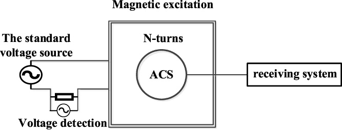
Simplified block diagram of calibration system.

As shown in Fig. 5, in order to calibrate the corresponding frequency response, this method only requires the calibration source and voltage measuring tool to realize the calibration process in the field. Moreover, through uncertainty analysis, the influence of secondary field and other interference fields on the total field is very small, which greatly reduces the dependence of the traditional method on the uniform calibration field. The size of the field source can be set through error calculation and analysis. Compared with the large-scale calibration instrument of the uniform field calibration method, the calibration source used in this method greatly reduces the cost. And this method can realize the calibration of large coil.

Calibration system of ground-airborne frequency domain electromagnetic detection and reception system mainly uses the standard magnetic source to generate a computable magnetic field, the standard source provides excitation current to the square magnetic source, the ACS is placed in the center of magnetic source, and the magnetic flux at the position where ACS is located changes to generate an induced voltage. Because the induced voltage value is relatively small, the receiver reads the electrical signal through the amplifier, and a current detection circuit is set between the standard source and the load to read the current.

From this, the value of calibration coefficient can be deduced. Although the field environment is complex, the rectangular magnetic source is relatively easy to realize. When we set the excitation frequency parameter, excitation voltage parameter, transmission wire frame turns and measure the excitation current, we can analyze the magnetic field generated by the magnetic source under different conditions. The purpose of this paper is to quickly obtain the calibration coefficient of the receiving system in the working environment and complete the calibration before the detection.

3.1. Relationship between frequency induced voltage and magnetic induction intensity

To calibrate the ground-airborne frequency domain electromagnetic system, the corresponding relationship between the magnetic field intensity of the ACS and the output voltage of the whole system should be considered at first.

According to Faraday’s law of electromagnetic induction, the induced electromotive force will be generated when the magnetic flux passing through the receiving coil changes.

Then the time domain voltage: $\begin{eqnarray}\displaystyle u=-\frac{d{\phi}_{m}}{dt}=-\frac{d}{dt}\int _{S}B\cdot dS. & & \displaystyle\end{eqnarray}$ (3.2)

Where Φ_m is the coil magnetic flux and B is the magnetic field strength.

Fourier transform is performed on both ends of Eq. (3.2) to obtain the induced voltage in frequency domain $\begin{eqnarray}\displaystyle V\text{} & =\text{} & \displaystyle -j{\omega}{\phi}_{m}({\omega})=-j{\omega}{\mu}_{0}\int _{S}H({\omega})\cdot dS\end{eqnarray}$ (3.3) $\begin{eqnarray}\displaystyle V\text{} & =\text{} & \displaystyle -j{\omega}{\phi}_{m}({\omega})=-j{\omega}{\mu}_{0}\int _{S}H_{ztotal}\cdot dS_{Z}.\end{eqnarray}$ (3.4)

When H _z is uniform, the induced voltage of a single turn coil can be expressed as $\begin{eqnarray}\displaystyle V=-j{\omega}{\phi}_{m}({\omega})=-j{\omega}{\mu}_{0}S_{Z}N_{T}H_{Z}. & & \displaystyle\end{eqnarray}$ (3.5)

Where N _T is that numb of turns of the magnetic source calibration system.

The multi-turn coil induces voltage is: $\begin{eqnarray}\displaystyle V=-j{\omega}{\phi}_{m}({\omega})N_{S}=-j{\omega}{\mu}_{0}N_{S}S_{Z}N_{T}H_{Z}. & & \displaystyle\end{eqnarray}$ (3.6)

Where N _S is that numb of turns of the ACS to be calibrate.

Measured induced voltage collected by receiver after amplification by differential amplifier: $\begin{eqnarray}\displaystyle V_{R}\text{} & =\text{} & \displaystyle N_{S}A({\omega},R,C,L)\ast V=-j{\omega}{\mu}_{0}S_{Z}N_{S}A({\omega},R,C,L)N_{T}H_{Z}\nonumber\\ \displaystyle \text{} & =\text{} & \displaystyle -j{\omega}{\mu}_{0}S_{Z}N_{S}A_{1}({\omega},R,C,L)A_{2}({\omega},R,C,L)N_{T}H_{Z}.\end{eqnarray}$ (3.7)

Where A is the magnification of the receiving system, A ₁(ω, R, C, L) is the magnification of the ACS system (Including differential amplifier), A ₂(ω, R, C, L) is that magnification of the receiver.

A (ω, R, C, L) is a complex coefficient. In practical application, the influence of inductance, capacitance and resistance of the coil itself is usually ignored, which leads to measurement error.

When H _z is uneven, the theoretical induced voltage of single turn coil is: $\begin{eqnarray}\displaystyle V=-j{\omega}{\phi}_{m}({\omega})=-j{\omega}{\mu}_{0}N_{T}\int _{S}H_{Z}\cdot dS. & & \displaystyle\end{eqnarray}$ (3.8)

After N _S turns of coil pass through amplifier and receiver: $\begin{eqnarray}\displaystyle V_{R}=N_{S}A({\omega},R,C,L)\ast V=-j{\omega}{\mu}_{0}N_{T}N_{S}A({\omega},R,C,L)\int _{S}H_{Z}\cdot dS_{Z}. & & \displaystyle\end{eqnarray}$ (3.9)

The calculation method of the calibration coefficient and the amplification factor of the receiving system can be derived from the formula. (3.9): $\begin{eqnarray}\displaystyle K={\omega}S_{Z}N_{S}A({\omega},R,C,L)=\frac{V_{R}\cdot S_{Z}}{-j{\mu}_{0}N_{T}\int _{S}H_{Z}\cdot dS_{Z}}. & & \displaystyle\end{eqnarray}$ (3.10)

K is defined as the calibration coefficient of the system. It is used to reflect the relationship between the measured induced voltage and the real magnetic field value of the ground-airborne frequency domain electromagnetic detection and receiving system. Every ground-airborne frequency domain electromagnetic detection and receiving system has a unique corresponding K when collecting signals with different frequencies. In actual detection, we can obtain more accurate magnetic field intensity values and know the deviation of the whole system from the theoretical value more intuitively by obtaining an accurate K value. According to formula (3.10), K contains multiple variables, for each detection system that has been come into service, S _Z, N _S, ω, μ₀, N _T are known values and V _R, H _Z are to be evaluated. When the K value of each frequency point in different receiving systems is uniquely determined, we can directly use the K value to correct the data in the later data processing process. In this paper, when the actual induced voltage value of the ACS and measured induced voltage collected by receiving system are acquired by calibration, the magnification of the system A can be calculated according to formula (3.9), and then acquire the K value.

4. Uncertainty analysis

The calibration system used to calibrate the ground-airborne frequency domain electromagnetic detection system has been described above, and the calibration coefficient of the ground-airborne frequency domain electromagnetic detection system can be calculated by (3.10). However, due to the existence of measurement errors, the complete calibration result includes not only the measured value, but also the uncertainty in the measurement process, so as to express the uncertainty of the measured value, which determines the calibration capability of the calibration system.We evaluate the reliability of the system by evaluating the uncertainty of ACS induced voltage. We can directly obtain the value of V about the receiving system by calibration. So the next crucial step is to evaluate the expanded uncertainty U of K, U is get from multiplying the combined standard uncertainty $U_C(V)$ by covering factor k (usually equals to 2), and U _C(V ) is a synthesis of multi-standard uncertainties [u (x ₁), u (x ₂), …u (x _i)], which come from all possible error sources that influence the calibration accuracy. Through Eq. (2.6) and Eq. (3.10), the error sources can be identified, including the turns of magnetic source and ACS, the side length of magnetic source and the radius of ACS, the relative position of magnetic source and ACS, measurement of excitation current, the height of ACS, the influence of earth resistivity, environmental magnetic noise and instrument noise.

4.1. Magnetic source turns and ACS turns (N _T and N _S) error

For the magnetic source excitation used in the calibration system in this paper, because of the receiving and transmitting distance is relatively close, if a multi-turn coil is wound, the signal of the receiving system to be calibrated will be saturated easily when the excitation current is small, and when the number of turns increases, it is difficult to determine the equivalent area of the magnetic source because the areas surrounded by different turns are difficult to be equal. Indirect measurement may be needed to determine the equivalent area of the magnetic source. In order to avoid complicated measurement and improve accuracy, it is best to minimize the number of turns. In this system, the turns of magnetic source is 2. The ACS is an accurately wound 300-turn silver-plated copper wire, so there is no turn error. Therefore, the standard uncertainties u (x ₁) and u (x ₂) of the number of turns error of magnetic source and ACS can be ignored.

4.2. Side length of magnetic source and radius of ACS (2a and D∕2) error

The magnetic edge length is measured by a precision π ruler, which is usually used to measure the circumference of a precision round workpiece. The π ruler used in this paper is made of elastic steel belt, and its measuring range is 1900–2125 mm. The two ends are engraved with a main ruler and an auxiliary ruler, and the minimum division value of the auxiliary ruler is 0.02 mm According to the data table given by the manufacturer of π ruler, the indication error of this ruler is ±0.08 mm. When calculating the uncertainty u (x ₃) caused by the side length of the magnetic source to the induced voltage, it is considered that each error is within the indicated error range.

As shown in Fig. 6, the ACS is a 300-turn silver-plated copper wire with a cross-sectional area of 1.13 × 10⁻⁷ m² wound on a nylon skeleton with a diameter of 0.45 m in the groove, and the outer diameter of the wire is about 0.38 mm. The width l of the two wire slots is 10 mm, because they are wound close to the coil frame, the maximum radius error of the ACS is 6 times of the outer diameter of the wire, that is, 2.28 mm, and the maximum radius error of the ACS is 1.01% compared with the ACS radius of 0.225 m. Figure 7 shows the influence of ACS radius on induced voltage, which is very tiny within the radius error range. The uncertainty of radius to induced voltage is represented by u (x ₄).

Fig. 6.

The coil skeleton is made of nylon, which is wound in two sections, forming a differential structure indirectly, effectively suppressing the common-mode noise and reducing the distributed capacitance of the coil. The inner diameter of the coil slot is D, the average diameter of the coil is d, the winding height is h, and the slot width is l.

Fig. 7.

The calibration system parameters are excitation current of 0.0193 A, 512 Hz, and earth resistivity of 100 𝛺 ⋅ m. At this time, the induced voltage of ACS is affected by the equivalent area of ACS, and increases with the increase of radius, but when the radius is within the error range, the change of V is in the order of 10⁻⁹ magnitude.

4.3. Magnetic excitation current

The parasitic capacitance of the power resistor connected in series between the signal generator and the magnetic source is less than 0.3 pF, and its resistance value is 2 Ω, so it shows resistance characteristics in the frequency range of 0.1–10 KHz calibrated in this paper. Therefore, the standard uncertainty of the measurement error u (x ₅) of the excitation current comes from the technical data sheet of the manufacturer of the current detector, namely the oscilloscope DPO2014B.

4.4. Height of ACS

The working principle of the ACS is well known. When the magnetic flux of the closed circuit changes, the induced current will be generated in the closed circuit. If we assume that the magnetic flux density to be measured is sine wave, the output voltage is proportional to the magnetic flux density B. When the ACS is in the calibration state, when the ACS is equivalent to 300 turns of wires evenly wound at a height of 0–20 mm, the height of the ACS is parallel to the Z axis of the magnetic field. Because the magnetic field is not uniform, the wires at different heights will produce different induced currents, which will affect the measurement results. To simplify the calculation, it is assumed that ACS is a conductor at any height point I within the height range, and the induced voltage is V _i. The uncertainty of height u (x ₆) to induced voltage is calculated by the A-type uncertainty calculation method. However in practical application, through the analysis of Fig. 8, It can be considered that ACS is in the range of uniform magnetic field value at half the height of the ACS, which is h/2.

Fig. 8.

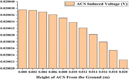
Changes of induced voltage within the range of ACS height.

4.5. Earth resistivity

The resistivity mainly affects the earth reflection coefficient r _TE, which is a variable that affects the magnetic induction intensity. The uncertainty of resistivity to induced voltage is calculated by calibrating the system model, and the earth resistivity in the area where the system works is 40–100 Ω ⋅ m. The ACS induced voltage with different resistivities is calculated by numerical analysis, and the sensitivity coefficient of uncertainty u (x ₇) is determined by the influence of resistivity on ACS induced voltage. As can be seen from Fig. 9, in the calibration system in this paper, the magnetic source is used as a device to excite the magnetic field in space. Because the distance between the transmitter and receiver is very close, the secondary field reflected by the earth is small compared with the primary field with high amplitude. Although the change of earth resistivity will affect the intensity of the secondary field, it has relatively little impact on the induced voltage of ACS.

Fig. 9.

Changes of ACS induced voltage in the range of earth resistivity.

4.6. Environmental magnetic noise

Due to the interference of nearby electrical equipment, power frequency noise, geomagnetic field and the influence of the instrument itself, when the magnetic source measurement system is not excited, the data read by the receiver is regarded as the sum of all the noises affecting the ACS, which determines the standard uncertainty u (x ₈). In order to reduce this uncertainty, the measuring system should keep a large enough distance from unexpected magnetic field sources (such as transformers and receivers) when working. Also the wires connected to the magnetic source should be twisted to avoid other magnetic flux injection.

In the urban environment, collect several groups of measured data of receiver without excitation to simulate the situation of maximum noise. The result is shown in Fig. 10. When the noise is less than one thousandth of the induced voltage of the ACS, the influence of noise on the signal is ignored. From Table 1 can be seen that in the frequency range of the receiving system, the noise has the greatest influence in the range of 512–2048 Hz. It is our key consideration in simulation calculation to determine the side length of magnetic source excitation according to the noise. Therefore, a magnetic excitation coil with two meters side length is set. When excitating with two meters side length, the error caused by environmental noise is less than 0.1%.

Fig. 10.

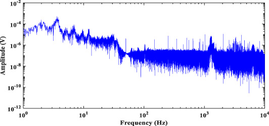
One of the empty mining experiments in urban environment. the amplitude-frequency curve of noise.

Table 1

Empty mining experiment data

Frequency (Hz)	Empty mining voltage (V)	Voltage at 2 m side length (V)
16	2.056 × 10⁻⁶	5.271 × 10⁻³
32	2.636 × 10⁻⁶	9.74 × 10⁻³
64	4.203 × 10⁻⁵	1.882 × 10⁻²
128	5.738 × 10⁻⁵	4.203 × 10⁻²
256	2.846 × 10⁻⁵	8.486 × 10⁻²
512	1.57 × 10⁻⁴	1.697 × 10⁻¹
1024	2.021 × 10⁻⁴	8.448 × 10⁻²
2048	1.459 × 10⁻⁴	1.659 × 10⁻¹
4096	4.93 × 10⁻⁵	3.095 × 10⁻¹
8192	6.412 × 10⁻⁶	4.891 × 10⁻¹

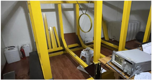
The mathematical model for assessing the combined uncertainty can be expressed by Eq. (4.2). Here V ^′ is an improved expression of V after considering u (x ₈), the independent variable x _i is correspond to each influence quantity (N _T, N _S, …, V _N), V _R means corrected value due to the change of earth resistivity, V _N means corrected value due to environmental magnetic noise. $\begin{eqnarray}\displaystyle V^{\prime }=F(x_{1},x_{2},\ldots ,x_{10})\text{} & =\text{} & \displaystyle F(N_{T},N_{S},2a,D/2,I,h,V_{R},V_{N})\nonumber\\ \displaystyle \text{} & =\text{} & \displaystyle {\omega}{\mu}_{0}IN_{S}N_{T}S_{Zi}H_{Zi}+V_{R}+V_{N}.\end{eqnarray}$ (4.1) Therefore, the combined standard uncertainty is given by $\begin{eqnarray}\displaystyle u_{c}^{2}(V^{\prime })=\mathop{\sum }_{xi}^{2}C_{xi}^{2}u^{2}(x_{i}) & & \displaystyle\end{eqnarray}$ (4.2) where $\begin{eqnarray}\displaystyle C_{xi}=\left(\frac{\partial F(x_{1},x_{2},\ldots ,x_{8})}{\partial x_{i}}\right). & & \displaystyle\end{eqnarray}$ (4.3)

5. Comparison between magnetic excitation calibration and other method

We have established a field calibration system based on magnetic source excitation. This system is applied to the ground-airborne frequency domain electromagnetic detection receiving system developed by our laboratory. The receiving system is mainly applied to the exploration of the earth structure in complex terrain areas. In the calibration system, the AC signal input to the magnetic source comes from the function generator AFG3022C, which can generate a low distortion sine wave of at least a few volts, a few millihertz to a few megahertz. The internal resistance of the function generator is 50 ohms or even higher, which limits its output power. When connected to a magnetic source, it cannot generate a large current, and the impedance will increase with frequency. To improve the signal-to-noise ratio, the operational amplifier LT1028 with low voltage noise is selected to form the differential amplifier circuit. The oscilloscope DPO2014B is connected in parallel at both ends of the resistor and store data through the USB port. The receiver system of the ground-airborne electromagnetic detection system in frequency domain uses PC104 industrial computer as the main control system to control the whole system. Windows XP system is installed in the industrial computer, and the control software is written. It sends commands to the lower computer through the software and USB controller. The system has complete functions and man-machine interaction, and collects data at a sampling rate of 32 kHz. The measuring equipment used in the proposed calibration system is shown in Fig. 11.

Fig. 11.

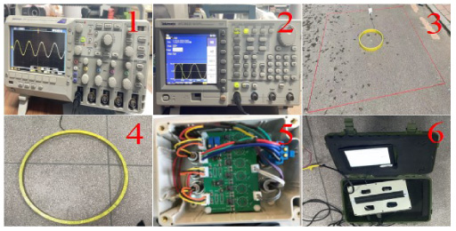
Receiving system to be calibrated and part of measuring equipment: 1. The oscilloscope DPO2014B 2. The function generator AFG3022C 3. The magnetic excitation 4. The ACS 5. The differential amplifier 6. The receiver.

5.1. The field experiment process of this method

The magnetic field generated by magnetic excitation is calculated as follows. Firstly, the electromagnetic field of line source was solved by Gaussian integration, and the number of turns, radius and height from the ground of the ACS were set, and the excitation coil parameters, including excitation frequency, excitation current and the number of turns of the transmitting coil, were set. Set underground medium parameters, including resistivity, resistivity thickness and permeability of each layer of two layers of earth, and finally call one-dimensional forward formula to calculate the induced voltage of receiving coil. A two-layer earth model is used to simulate the uniform earth, and the magnetic field generated by the magnetic source used for calibration and the induced voltage of the ACS are calculated.

The whole measuring process of is shown in Fig. 12. When calibrating the receiving system, the sensor induced voltage is read by the receiver. When the system excitation voltage value is determined to be a certain value, the calibration coefficient of the whole system can be determined by accurately reading the ACS induced voltage value. Experiments are conducted outdoors to simulate the field calibration environment. For the convenience of calculation, the transmitting wire frame is a square with a side length of 2 m, and wind the wire with two turns to increase the effective area. The magnetic source is laid on the ground, the ACS is used as the receiving coil, and the center of the coil is placed at the center of the transmitting wire frame. The high-precision signal generator provides voltage for the magnetic source and the low frequency band (16–512 Hz) gives 8V excitation signal (because of the differential input of the signal generator, the signal generator displays 4 V). As the frequency increases, the sensitivity coefficient of the ACS increases, which is easy to reach saturation. Therefore, the high frequency band (512–8192 Hz) is given a 2 V excitation signal (the signal generator displays 1 V). The voltage source outputs voltage signals of different frequencies, drives the receiving coil as an inductive load, connects a power resistor with a resistance of 2 Ω in series between the signal generator and the rectangular transmitting wire frame, and records the effective voltage values at both ends of the resistor through the oscilloscope to calculate and record the exciting current, also records the voltage peak-to-peak values at both ends of the resistor by the portable digital oscillograph (overlapping 512 times), so as to ensure reliable excitation current result. The ACS connected to the receiver through the amplifier. Table 2 gives the calibration uncertainty value of the calibration system at 512 Hz and 0.028027 V, sensitivity coefficient C _xi is get by calculating partial derivative, the relative expanded uncertainty U _rel is estimated as 1.48% while the absolute value U is 0.000041 V, for k = 2.

Fig. 12.

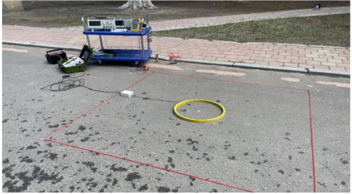
Testing outdoors.

Table 2

Uncertainty budget list of ACS induced voltage 0.028027 V at 512 Hz

Standard uncertainty component u (x _i)	Soure of uncertainty	Sensitivity coefficient C _xi	Relative standard uncertainty \|C _xi \| u (x _i)
u (x ₁)	Magnetic source turns N _T	0.014	0
u (x ₂)	ACS turns N _S	0.00009	0
u (x ₃)	Side length of magnetic source 2a	0.029	0.001%
u (x ₄)	Radius of ACS D∕2	2.24	0.012%
u (x ₅)	Exciting current I	0.177	4%
u (x ₆)	Height of ACS h	0.0008	0.00045%
u (x ₇)	Earth resistivity V _R	0.0000001837312	0.000000078%
u (x ₈)	Environmental noise V _N	1	0.0045%
Relative combined uncertainty			0.74%
Relative expanded uncertainty	U _rel (k = 2)		1.48%
Absolute expanded uncertainty	U (k = 2)		0.000041 V

From the Table 3, it can be seen that the system amplifies the signals of different frequencies to varying degrees. If the instrument is not calibrated, the high-frequency amplitude measurement value is too small, and the calibration coefficient for 64 Hz is obviously smaller, which is due to the influence of the 50 Hz trap in the preamplifier circuit on nearby frequencies. Therefore, system calibration is very important to ensure the accuracy of data.

Table 3

Results of outdoor experimental

Frequency f (Hz)	ACS induced voltage V (V)	Absolute expanded uncertainty U	Measured voltage V _R (V)	Calibration coefficient K
16	0.000877388	0.000002 V	0.005271	6.007602239
32	0.001751698	0.000004 V	0.00974	5.560318960
64	0.003503396	0.000007 V	0.01882	5.371930335
128	0.007006792	0.000013 V	0.04203	5.998201129
256	0.014013584	0.000026 V	0.08486	6.055552775
512	0.028027168	0.000041 V	0.1697	6.054839313
512	0.007092992	0.000011 V	0.04245	5.984780801
1024	0.014136725	0.000021 V	0.08448	5.975924210
2048	0.028273446	0.000042 V	0.1659	5.867696470
4096	0.056743893	0.000085 V	0.3095	5.454331487
8192	0.115457905	0.000169 V	0.4849	4.199799064

5.2. Verify the performance of the calibration system by calibrating ACS

In order to verify the performance of the above-mentioned measurement system, the measurement results are compared with the method of generating standard field through Braunbeck coil calibration system in the shielded room (see Fig. 13). As the calibration method described in this paper is mainly used to obtain the calibration coefficient of the receiving system at the project site, the influence of environment on the experimental results can’t be estimated. As Agilent35670A dynamic signal analyzer is easy to saturate and can’t realize large excitation signal, the comparison method verifies the reliability of the above-mentioned measurement system by obtaining the sensitivity coefficient of ACS at different frequencies. In Braunbeck coil calibration system, the Braunbeck coil is excited by keithley current source, and the electric signal induced by ACS is read by Agilent35670A dynamic signal analyzer, and the same ACS is calibrated at the corresponding frequency. The contrast experiment was conducted in an electromagnetic shielding room, and the calibration conditions met the environmental requirements. Table 4 shows the calibration results of ACS by magnetic source excitation calibration system and Braunbeck coil calibration system. In the 0.1 Hz–10 kHz frequency band, ACS sensitivity is basically linear with frequency, and the measured values of the two methods are basically consistent, but there is a significant deviation at high frequencies. The high-frequency measurement result of the Braunbeck coil calibration system is obviously high. We think that there are two main reasons for this error, one is the measurement error of differential amplifier and receiver amplification in the receiving system, the other is the noise error of the shielded room environment and the field environment, meanwhile, the uncertainties of the two calibration systems are different. It can be concluded that the calibration system based on magnetic source excitation is reliable and can basically meet the requirements of receiving system calibration in the project site.

Fig. 13.

Calibration of ACS by Braunbeck coil.

Table 4

Results of outdoor experimental

Frequency (Hz)	Magnetic excitation calibration system ACS sensitivity (mV/nT)	Frequency (Hz)	Braunbeck coil calibration system ACS sensitivity (mV/nT)
16	0.0040081	16	0.003949725
32	0.008002137	32	0.007818619
64	0.015966259	64	0.015437239
128	0.031932517	128	0.030484817
256	0.063940973	256	0.06145683
512	0.129378943	512	0.125055072
1024	0.255730761	1024	0.23569322
2048	0.511612174	2048	0.484271269
4096	1.023170459	4096	1.171786283
8192	2.055962892	8192	2.218803952

6. Conclusions

In this paper, basing on the method of Magnetic excitation, a measurement system for ground-airborne frequency domain electromagnetic detection receving system calibration in the frequency range from 0.1 Hz to 10 kHz has been described.

Compared with traditional calibration, magnetic source excitation method can effectively avoid the influence of environmental noise and other factors on calibration results, and it is an effective way to improve the instrument accuracy of electromagnetic ground-penetrating measurement system in ground-airborne frequency domain.

The uncertainty of calibration system based on magnetic source excitation in frequency range is analyzed. Consequently, the evaluated expanded uncertainties are from 0.7% to 1.1% for k = 2. Compared with other calibration methods, the performance of the measurement system is verified. The experimental results show that, compared with the traditional frequency response method, there is no need to provide a uniform magnetic field, and there is no need to tailor the equipment for generating a uniform magnetic field according to the shape of the ACS. For the subsequent field experiments, the calibration of large-scale ACS is of great significance. In the future application, in order to expand the application range of electromagnetic detection methods in the ground-airborne frequency domain, larger sensors will be widely used to improve detection efficiency and increase application scenarios. The frequency response calibration of large sensor will be carried out based on the research content of this paper.

Footnotes

Acknowledgement

This work was supported by Natural Science Foundation of Jilin Province [grant number 20220101169JC]，National Natural Science Foundation of China [grant number 42174085，41904159].

References

Xue

G.Q.

, The development of near-source electromagnetic methods in China, Journal of Environmental and Engineering Geophysics 23(1) (2018), 115–124, doi:10.2113/Jeeg23.1.115.

Lin

Kang

L.L.

Liu

C.S.

Ren

T.Y.

Zhou

H.G.

Yao

, The frequency-domain airborne electromagnetic method with a grounded electrical source, Geophysics 84(4) (2019), E269–E280, doi:10.1190/Geo2017-0777.1.

Zhou

H.G.

Lin

Liu

C.S.

Kang

L.L.

and Zeng

X.S.

, Interaction between two adjacent grounded sources in frequency domain semi-airborne electromagnetic survey, Review of Scientific Instruments 87(3) (2016), Artn 034503, doi:10.1063/1.4943221.

Smith

R.S.

and Balch

S.J.

, Robust estimation of the band-limited inductive-limit response from impulse-response TEM measurements taken during the transmitter switch-off and the transmitter off-time: Theory and an example from Voisey’s Bay, Labrador, Canada, Geophysics 65(2) (2000), 476–481, doi:10.1190/1.1444741.

C.G.

Z.H.

Zhang

H.Q.

Tai

H.M.

and Zhu

X.G.

, Transient process and optimal design of receiver coil for small-loop transient electromagnetics, Geophysical Prospecting 62(2) (2014), 377–384, doi:10.1111/1365-2478.12093.

Wang

H.W.

Z.H.

Wang

Tai

H.M.

and Chen

W.L.

, On-site calibration of air-coil sensor for transient electromagnetic exploration, Geophysical Prospecting 67(6) (2019), 1595–1610, doi:10.1111/1365-2478.12737.

Kozhevnikov

N.O.

, Testing TEM systems using a large horizontal loop conductor, Russian Geology and Geophysics 53(11) (2012), 1243–1251, doi:10.1016/j.rgg.2012.09.010.

Persova

M.G.

Soloveichik

Y.G.

Trigubovich

G.M.

Vagin

D.V.

and Domnikov

P.A.

, Transient electromagnetic modelling of an isolated wire loop over a conductive medium, Geophysical Prospecting 62(5) (2014), 1193–1201, doi:10.1111/1365-2478.12122.

Davis

A.C.

and Macnae

, Quantifying AEM system characteristics using a ground loop, Geophysics 73(4) (2008), F179–F188, doi:10.1190/1.2943189.

10.

F.M.

Chen

Z.P.

Zhu

L.Z.

Liu

Wang

Z.J.

and Zhuang

, Note: A calibration method to determine the lumped-circuit parameters of a magnetic probe, Review of Scientific Instruments 87(6) (2016), Artn 066102, doi:10.1063/1.4953240.

11.

Gurleyuk

S.S.

Taskin

and Sarac

, Measurement of the parameters and the resonance frequency in semiconductor controlled Tesla transformer, International Journal of Electrical Power & Energy Systems 43(1) (2012), 6–10, doi:10.1016/j.ijepes.2012.05.026.

12.

Lin

Wang

X.G.

Cai

and Shang

X.L.

, Research and development on the air-core coil sensor for mine transient electromagnetic exploration, Chinese Journal of Geophysics-Chinese Edition 59(2) (2016), 721–730, doi:10.6038/cjg20160229.

13.

Rubens

S.M.

, Cube-surface coil for producing a uniform magnetic field, Rev. Sci.Instrum. 16(9) (1954), 243–245.

A calibration method of ground-airborne frequency domain electromagnetic receving system based on magnetic source excitation

Abstract

Keywords

1. Introduction

2.1. Layered earth simulation model

4.1. Magnetic source turns and ACS turns (N T and N S ) error

4.2. Side length of magnetic source and radius of ACS (2a and D∕2) error

4.4. Height of ACS

Footnotes

Acknowledgement

References

4.1. Magnetic source turns and ACS turns (N _T and N _S) error