
Abstract
In modern wireless telecommunication systems, antenna arrays are widely used as elements of multiple – input multiple – output technology. In the fifth-generation systems, arrays are utilized to realize beamforming that forms the radiation pattern of the base station in the direction of the mobile user. This requires the utilization of many-element antenna arrays that are precisely controlled to achieve the required radiation properties. In this paper we apply the concept of deep neural network to model antenna array radiation properties. In this proof-of-concept research we aim at investigating to what extent it is possible to use deep neural networks for modeling antenna arrays. We consider a full-wave model of linear array with a reflector, which was controlled by the phase and amplitude of the signals feeding the elementary radiators. The applied method made it possible to solve the direct and inverse problems. The results that we obtained show that deep neural networks are able to model antenna array properties.
Introduction
Wireless communication systems are constantly evolving towards greater capacity and data throughput. Their successive generations are characterized by an increasing speed of data transmission (data rate) and user density as well as lower latency and improved power efficiency. For this purpose, it is necessary to develop new technologies to enable the achievement of these goals. In recent years, the so-called fifth-generation (5G) of wireless systems was introduced [1]. Unlike its predecessors, it uses very complex antenna systems that are able to dynamically shape their radiation patterns. In 5G systems, massive multiple – input multiple – output (MIMO) technology benefits from the utilization of antenna arrays [2]. These are antenna systems composed of many radiators, which, depending on the phase shift and the amplitude of the signal feeding each radiator, change the radiation pattern [3]. Beamforming is a technique that is used to control antenna arrays. It improves the efficiency and capacity of wireless communication systems by focusing the transmission and reception of signals along specific directions. This allows the synthesis of unique radiation patterns by varying the amplitude and phase of the signals supplied to each antenna element in the array. Several patterns can be used to transmit the signal in the directions of users. This concept is shown in Fig. 1 where the antenna array at the base station forms two different beams to transmit data from two users. Beamforming expands coverage, enhances signal quality, and reduces interference. For this purpose advanced algorithms are used to examine the signal strength and quality of the link between the device and the network [4,5]. The development of beamforming algorithms requires the utilization of antenna array models that can handle physical effects that occur in real antenna systems. The antenna array element coupling and reflector performance as well as array imperfections influence the radiation properties of the whole system [6]. Modeling of antenna arrays is therefore important from the point of view of the development of communication systems that are using beamforming techniques.
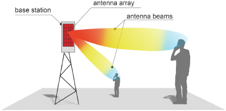
Antenna array in 5G system.
In this respect, a deep neural network (DNN) is a type of artificial neural network (ANN) that has multiple layers of interconnected nodes (neurons) inspired by the structure and function of the human brain [7–9]. Deep neural networks have achieved remarkable success across various domains, including computer vision, natural language processing, speech recognition, and reinforcement learning. They were also successfully applied in electromagnetic problems [10,11], including antenna array pattern synthesis [12]. DNN was also applied to the implementation of antenna array beamforming [13] for different antenna array configurations [14].
In general, there have been many recent contributions using machine learning (ML) to accelerate the design process of microwave components. Three major categories may be recognized among them: forward, inverse, and generative ML methods, respectively. The main difference is that forward ML models aim at finding the electromagnetic response of a component to design parameters [15,16], while inverse models do the opposite [17,18]. In turn, generative ML models learn the statistical distribution of design parameters and then are able to generate unseen parameter settings [19,20]. Moreover, generative ML models are often integrated with forward models for evaluating the response to new parameter settings.
In this paper we apply DNN to develop the parametrized model of the antenna array. The research presented in [12] proved the ability of DNN to model antenna array radiation pattern; however, this had to be described by a multidimensional vector of antenna elements excitation parameters. In that research a randomly generated excitation parameters were used to examine antenna performance. In our approach, in contrast, we used an efficient way to describe the parameters of the antenna array. Here the dimension of the problem is reduced to 2 parameters: the subsequent phase shift on each radiator, and the parameter controlling the amplitude distribution in the antenna array. As the output, instead of radiation patterns in three dimensions, we use the direction of the main beam and the sidelobe level. This approach to the problem allows us to effectively use the developed network in order to model the antenna array implementing the beamforming algorithm in modern 5G systems.
In the further part of the article, the method of linear antenna array modeling using the Matlab Antenna Toolbox is presented. It was used to generate training data for the neural network. In the following, the network topology, its learning process and the results obtained are described.
Antenna arrays have been used for many years in antenna technique to realize directional radiation patterns with electrically controlled properties [3]. Due to the fact that the array radiation pattern depends on the amplitude and phase of the signals supplying elementary radiators, it is possible to form it by changing these parameters. The analysis of the antenna array can be performed with simplified relations that describe the radiation properties of the array as a combination of the radiation pattern of a single element and the array factor that is a function of the geometry of the array and the excitation phase of signals [3]. This approach, however, does not take into account the electromagnetic coupling between the radiators and the influence of the metallic reflector of finite size. Another approach uses electromagnetic simulations based on Maxwell’s equations. In this case, any radiator geometry can be included. Also, the couplings between elements are taken into account and the reflector can be properly modeled. In our research, we used the latter approach; in particular, we have utilized Matlab Antenna Toolbox for visualization of the antenna and subsequent array field analysis [21]. This allows the use of prefabricated antenna elements with parametric geometry, arbitrary planar structures, or unique 3D structures. In this toolbox the method of moments (MoM) is used to calculate antenna impedance, current distribution, efficiency, and near-field and far-field radiation patterns [22].
For the sake of simplicity, we here consider the linear antenna array with different number of radiators, formed by half-wave dipoles. As far as the case study is concerned, the 4-element array is presented in Fig. 2. We assume that the antenna operates on 3.5 GHz frequency, a typical value that is assigned in many countries for 5G systems. The length of dipoles is 39.5 mm while their width is 2 mm; moreover, the element spacing in the x direction is 42.9 mm and it is equal to half of the wavelength. Eventually, the reflector spacing from the dipoles in the z direction is 12.9 mm that corresponds to 0.15 of the wavelength. We assume that the reflector is larger than the area of the radiators in the x-direction by
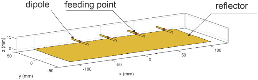
Geometry of linear antenna array made of 4 dipoles with planar reflector.
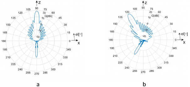
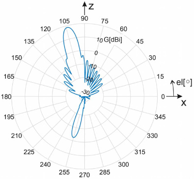
The radiation pattern of the considered array depends on many parameters. The greater the number of elements, the narrower the main beam of the pattern and the greater the maximum gain of the array. Increasing the number of elements also increases the number of sidelobes. This is shown in Fig. 3 in the form of 3D plot and in Fig. 4 in the polar plot in the elevation plane (x--z cut). The change in the phase shift of the signals applied to the subsequent elements results in tilting the beam of the main antenna. This is shown in Fig. 5. In our case of linear array we apply a cumulative phase shift with the φ parameter which is the difference between phase shift between two subsequent elements.
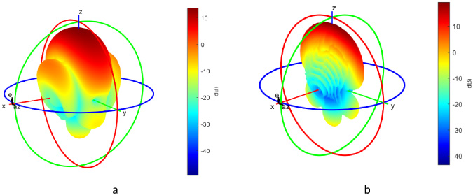
Radiation pattern of the linear antenna array: a – 4 elements, b – 16 elements.
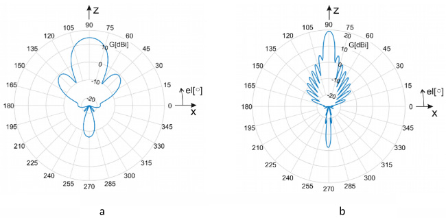
Radiation pattern of the linear antenna array in elevation plane: a – 4 elements, b – 16 elements.
Radiation pattern of the linear antenna array with 16 elements and different phasing: a – φ = 0°, b – φ = 90°.
The array radiation pattern depends on the phase of signals on each element as well as on their amplitudes. In the research presented in [12] the wide range of randomly generated phases and amplitudes was used for investigating the antenna for the sake of DNN training. Instead of this, in our case, the amplitudes of signals exciting the radiators are controlled by the parameter of the amplitude distribution function. In [23] excitation amplitudes based on Gaussian distribution were applied to enhance the radiation properties of a millimeter-wave patch array antenna operating at 30 GHz. For a linear array, the excitation amplitudes are samples of the function f (1):
This excitation function improved the radiation control compared to the uniform and traditional non-uniform excitation amplitudes [23]. In our case we assume a symmetrical distribution of signal amplitudes, considering σ as the parameter that controls the amplitudes of signals that are feeding elementary radiators of the antenna array. It is important to note that σ influences amplitudes of signals and so the directional properties of antenna array are strongly dependent on this. In Fig. 6 the influence of this parameter on antenna array radiation pattern is presented.
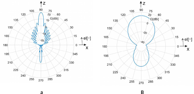
Radiation pattern of the linear antenna array: a – σ = 10, b – σ = 1.
The radiation pattern of the considered linear antenna array in x--z elevation plane is an angular distribution of antenna gain G (θ). This distribution can be characterized by several parameters, that are presented in Fig. 7. The direction of antenna maximum radiation is the main beam angle θ(G max ). It is the angle between the direction of the maximum of the major lobe and x axis. Another parameter that is important for antenna arrays is the side lobe level G s that is the maximum level of the sidelobes in dBi. For directional antennas it is desired to reduce this parameter.
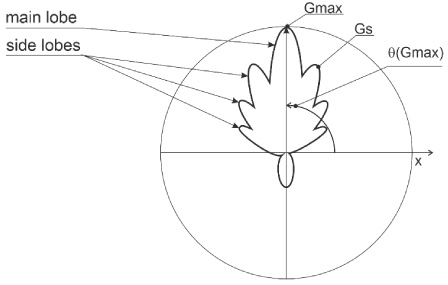
The parameters of radiation pattern.
The radiation pattern of the antenna includes the angular distribution of the gain values. This is a dense data set for the 3-dimensional case. When antenna modeling is performed with the use of neural networks, the amount of data we want to receive requires a similar number of input data necessary to train the network. Due to the fact that the data for network training comes from full-wave electromagnetic analyses, their number is limited due to the simulation time needed to obtain them. For this reason, in the following, we will describe the radiation pattern of the array using only two characteristic parameters such as main beam angle θ(G max ) and a sidelobe level G s (reference to Fig. 7).
The radiation pattern parameters (θ(G max ) and G s ) were obtained with MoM-based simulations for different values of φ and σ parameters. The values of θ(G max ) as the function of φ and σ are presented in Fig. 8, while values of G s are shown in Fig. 9. Simulations were carried out for 341 values of the φ parameter changing from −170° to 170° every 1° and for 10 values of the σ parameter changing from 0.5 every 0.5 step to 5. This resulted with a uniform, full-factorial like, sampling of parameter space in the range of their variability, which have the greatest impact on the antenna radiation, was developed. Accordingly, 3,410 simulations were performed with MoM based analyses. This task was possible thanks to a twofold condition: the high computational efficiency of MoM algorithm on the one hand, and the simple configuration of the antenna array on the other hand. Specifically, for 16 element array a single analysis lasted 50 s while for 32 element array it lasted 151 s on the computer equipped with Intel® Core i7-9850H CPU working with 2.60 GHz clock. As a result, the response surfaces of antenna radiation parameters are presented in Figs 8 and 9: thanks to the wide set of analyses, the surfaces are smooth and provide the ground-truth information about antenna array performance.
The unequal distribution of input parameters resulted from the fact that the φ parameter can vary in a large range and has a substantial influence on the main beam angle θ(G max ). The beam angle for a considered array with a reflector can change from approximately 30° to +150°. It was then necessary to study this dependence with high resolution to provide the necessary information for ANN data set. The σ parameter changes to a smaller extent and its significance for the direction of the main beam is much smaller. In fact, it mostly affects the sidelobe level which varies from 6 dBi to −8 dBi. In addition, the limitation of the number of combinations of input parameters also resulted from the need to limit the computational cost of full-wave simulations.
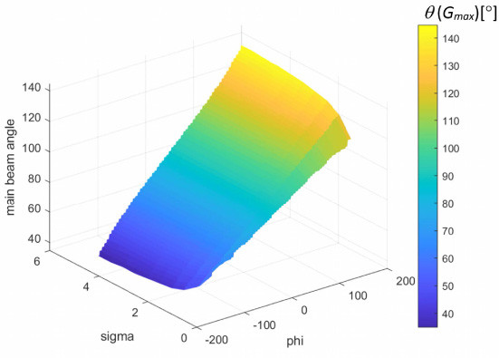
The values of θ(G max )[°] as the function of φ and σ.
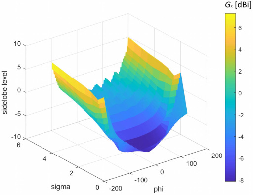
The values of G s [dBi] as the function of φ and σ.
The direct problem can be cast as follows: given array geometry, having prescribed shift angle and sigma parameter, find the corresponding beam direction angle and sidelobe level.
Before tackling a solution technique, a methodological preamble is necessary: metamodels of the direct problem are developed according to a concept of network decomposition; the reason is that the complete set of computed MoM responses can be difficult to approximate with a single network. Therefore, in the proposed ANN architecture, the learning task is distributed among a number of sub-networks, which divide the output space into a set of subspaces. In Fig. 10 a typical architecture of a fully-connected decomposed ANN is shown. In first case x vector consist of φ parameter and σ amplitude distribution parameter while S corresponds to main beam angle θ(G max ). In the second case S corresponds to sidelobe level G s .
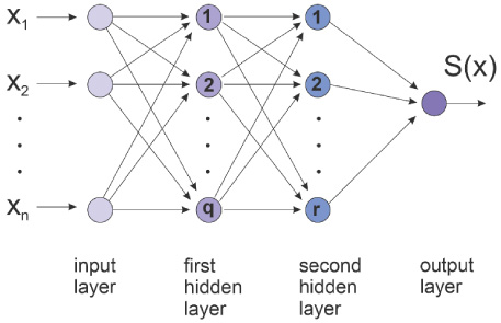
Exemplary architecture of a decomposed ANN.
Here a second methodological assumption comes in: it is supposed that for any allowable set of input variables, the response can be sufficiently obtained with the use of a single numerical simulation e.g., three-dimensional FDTD or, like in this paper, method of moments. With the use of these simulations, many samples of input-output pairs are generated in such a way that the training data set is governed by the following matrix:
For each neuron per layer, the output is computed as y = w t x + b, where x is the input vector, w t is transposed vector of weights (w1, w2, …, w n ), and b is a scalar bias.
In the paper feedforward networks for regression purposes are considered. In order a network to appropriately learn from examples, it was decided to make a partition of each data set according to the following criterion: 80% for training; 15% for validation; 5% for test. Then, weights and bias of each neuron are updated by means of Levenberg-Marquardt (LM) optimization, which is a fast back-propagation algorithm, although it requires a substantial use of memory. The governing equation of the method is the following:
and
Main beam angle θ(G max ) as a function of phase shift and sigma parameter: prediction vs ground truth (16-element array).
Main beam angle θ(G max ) (16-element array): convergence trends of the (80, 40, 20) network.
The following remark can be put forward: when 𝛼 = 0 the classical Newton’s method is recovered while in the limit of 𝛼 ≫1 the gradient descent takes place. As far as numerical aspects are concerned, the initial value of 𝛼 is set to 10−3, with a decrease factor of 0.1 and an increase factor of 10. Eventually, the rectified linear unit (ReLU) function was selected as the activation function per neuron.
It should be clarified that all numerical experiments here reported were achieved utilizing the Matlab Toolbox for Neural Networks. The loss function, defined as the quadratic discrepancy between predicted answer and true answer, was minimized by means of LM.
The rationale behind the LM scheme is that it is particularly well suited to the solution of non-linear problems. This is certainly the case of this research, where the relation between feeding signal parameters and antenna radiation parameters are non linear: it couild be appreciated looking e.g. at Fig. 9 which exhibits a remarkable non linearity in the dependence of sidelobe level on phase shift and amplitude distribution parameter.
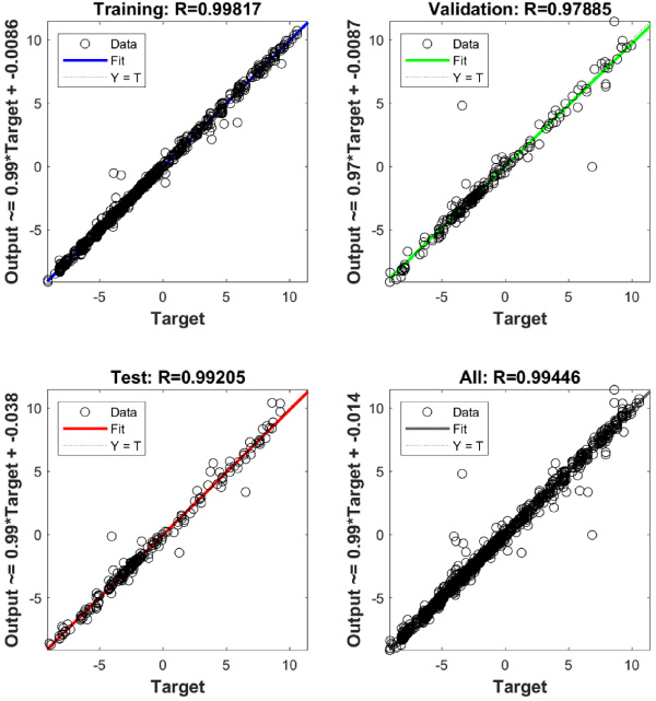
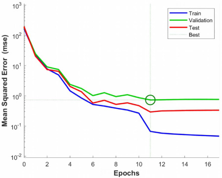
Moving from this background, a network predicting the main beam angle θ(G max ) as a function of phase shift and sigma parameter was first synthesized. The network is composed of three fully connected layers with (80, 40, 20) neurons, respectively; the training process was based on 1,000 data scanning phi in the range (−170°, +170°) and sigma in the range (0.5, 5); relevant results are shown in Fig. 11, while the relevant convergence trends are presented in Fig. 12.
In principle, in machine learning, dataset does not require normalization unless parameters exhibit different ranges. This is actually the case of phase shift and amplitude parameter for input data as well as main beam angle and sidelobe level for output data, respectively. In the paper, the min-max scaling technique was utilized in order to normalize the dataset before the training process.
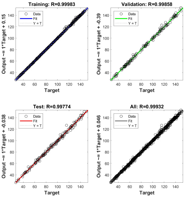
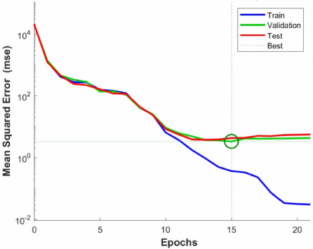
Subsequently, another (80, 40, 20) network was trained for predicting the sidelobe level G s , always in terms of phase shift and sigma parameters within the same ranges as above, with a training based on 1,400 data; the results obtained are shown in Fig. 13, while the relevant convergence trends are presented in Fig. 14.
Sidelobe level G s as a function of phase shift and sigma parameter: prediction vs ground truth (16-element array).
Sidelobe level G s (16-element array): convergence trends of the (80, 40, 20) network.
Both networks were then retrained for the case of 24-element array and also 32-element array, showing similar performances in their prediction ability.
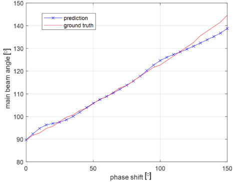
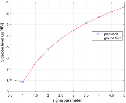
The network performance was tested for the wide range of φ parameter values. For the sake of an example, in Fig. 15 the results obtained using the network trained for 16-element array are presented. The main beam angle as the function of phase shift (ANN prediction) is in good agreement with results obtained with MoM (ground truth). Similar results hold for side lobe level in terms of sigma parameter (Fig. 16).
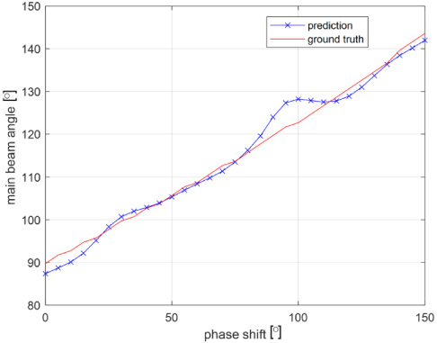
Main beam angle as the function of phase shift obtained for ANN (prediction) and MoM (ground truth) for 16 element array.
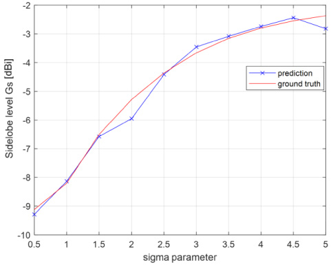
Side lobe level as the function of sigma parameter obtained for ANN (prediction) and MoM (ground truth) for 16 element array.
Moreover, the example of 16-element array radiation pattern obtained with MoM simulations for φ = 45° and σ = 5 is presented in Fig. 17. The parameters that were extracted from this simulations were the following: sidelobe level G s = −2.406 dBi, beam angle θ = 103.71°. The corresponding ANN predicted very similar values: the side lobe G s = −2.453 dBi, beam angle θ = 103.94°.
Example of 16-element array radiation pattern obtained with MoM simulations for φ = 45° and σ = 5.
Another example is presented for 32 element array. In Fig. 18 the main beam angle as the function of phase shift is presented. In this case prediction is in good agreement with ground truth up to the phase shift value of 130°. For phase shift that gets close to 150° the discrepancy between MoM and ANN is greater and reaches 5°. The results obtained for side lobe level in terms of sigma parameter (Fig. 19) are almost exactly the same for MoM and ANN.
Main beam angle as the function of phase shift obtained for ANN (prediction) and MoM (ground truth) for 32 element array.
Side lobe level as the function of sigma parameter obtained for ANN (prediction) and MoM (ground truth) for 32 element array.
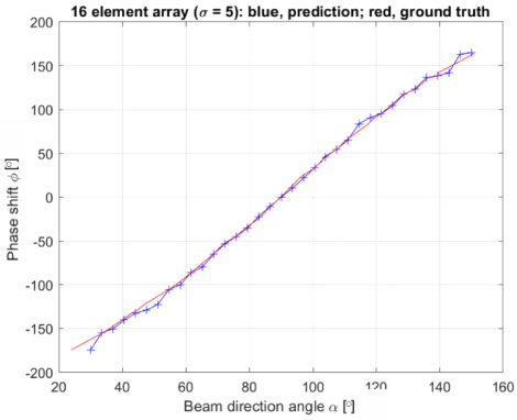
The inverse problem can be cast as follows: given array geometry, having prescribed the direction angle, find the corresponding shift angle and sigma parameter. To this end, a flipped network, i.e. a network exchanging the role of input and output with respect to its forward counterpart (Section 3), was next synthesized: it is able to predict shift angle given beam direction angle for several values of sigma parameters, with reference to the 16-element array. The network is composed of three fully connected layers with (80, 40, 20) neurons, respectively; the training was based on 2,000 data: for the sake of an example, the results obtained for σ = 5 are shown in Fig. 20. Indeed, the flipped network is a first approach towards a procedure of automated optimal design.

Flipped network: prediction vs. ground truth for φ parameter as a function of beam direction angle (16-element array, σ = 5).
Accordingly, a comparison between predicted and actual phase shift φ versus beam angle is shown in Fig. 21 exhibiting a reasonable agreement.
The results of flipped network that estimates sigma parameter given side lobe level were also caried out. In this case, the ground truth dataset obtained with MoM incorporates less datapoints compared to phase shift φ versus beam angle set. In Fig. 22 a comparison between predicted and actual side lobe level versus sigma parameter for 16-element array is presented (φ = 0°). It was obtained from ANN for G s ∈ [−9 : 0.5 : −2.5]. It can be noted that the discrepancies between the results obtained from ANN and MoM are greater here than for the flipped network used for phase shift estimation. Figure 23 presents similar results, however obtained for a different set of G s ∈ [−9 : 1.5 : −1.5]. In this case there is greater similarity between MoM and ANN results. This shows that the performance of the flipped network for σ estimation substantially depends on the set of input parameters used. This may be due to the smaller variability range of the sigma parameter (from 0.5 to 5) in the data used to train the network. Having limited number of training values combination, network cannot provide estimation that has sufficient similarity to the ground-truth data.
A comparison between predicted and actual phase shift versus beam angle for 16 element array.
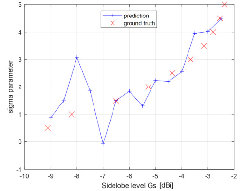
A comparison between predicted and actual side lobe level versus sigma parameter for 16 element array, φ = 0°. Results were obtained from ANN for G s ∈ [−9 : 0.5 : −2.5].
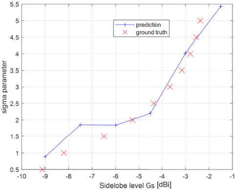
A comparison between predicted and actual side lobe level versus sigma parameter for 16 element array, φ = 0°. Results were obtained from ANN for G s ∈ [−9 : 1.5 : −1.5].
The upcoming wireless communication eras call for the speed-up and automation of the design process of microwave components: in this respect, machine learning shows a great potential for accelerating procedures of analysis and design. Accordingly, the paper has shown a proof of concept that ANN-based and MoM-backed approach to modeling can serve as a fast tool in designing a family of linear antenna arrays.
The original achievements of this work are the following. A parametric control of antenna array was successfully applied to antenna modeling with ANN. Moreover, a concept of decomposed ANN was utilized to solve direct problem. Eventually, a flipped ANN was synthesized to solve inverse problem of antenna array design.
The performance of the synthesized network for solving direct problem is very good. The results of antenna array radiation pattern approximation obtained from the ANN were very similar to results of full-wave electromagnetic simulations. Also the flipped network showed its high potential in fast and accurate approximation of antenna array feeding parameters. The task of finding the phase shift enabling the realization of the given main beam angle was solved with a very high accuracy. Identification of the value of the parameter controlling the amplitude (σ), which would make it possible to achieve the desired sidelobe levels, gave worse results. This may be due to the too limited range of this parameter in the data set used for the network training. Further work is being carried out on the development of a network that would have a satisfactorily good accuracy of approximation of this parameter as well.
While the functionality of most features depends on nature and complexity of the actual problem to solve, the paper illustrates the applicability of the proposed method to quite a diverse range of complex and electrically large systems, as well as their successful optimization.