Employing automatic differentiation and neural networks for parameter identification of an energy based hysteresis model

Abstract

This paper is about the parameter identification of an energy based hysteresis model from measurements by employing automatic differentiation and neural networks. We first introduce the energy based hysteresis model and the parameters which are to be identified. Then we show how the model can benefit from automatic differentiation. After that we incorporate a parametrization of the energy based hysteresis model via distribution functions and identify the parameters of the distribution function. Then, the hysteresis model is sampled and the generated datasets are used to train neural networks to predict the hysteresis parameters. The described methods are tested and verified on synthetic as well as measurement data.

Keywords

Optimization;parameter identification;hysteresis;machine learning;neural networks

1. Introduction

The problem of parameter identification [1] is one of the key burdens of developing realistic simulations. Even though precise models and measurement data are often present, the step from measurement data to model parameters is a challenging one. This can manifest itself in long optimization runs, very demanding computations or challenging parametrizations. In this paper we are dealing with the parameter identification of an energy based hysteresis model. One of the main challenges associated with the identification of energy based hysteresis model parameters is the dependency of the model expressivity on the number of parameters. The problem with a growing number of parameters is that the dimension of the optimization space is also growing linearly with it, which makes the whole identification process more difficult. Also, with a larger number of parameters, calculating the derivatives of the error function with respect to these becomes more expensive. Therefore in this work we focus on mitigating these issues while still preserving an accurate depiction of the measurements.

The paper is structured as follows. First, the energy based hysteresis model [2] is introduced where the origin and the role of the hysteresis model parameters are explained. Then we show how and why automatic differentiation [3], which is mainly used in the machine learning community, is employed in this context. In doing so, derivatives of the hysteresis model can be efficiently computed while allowing for simple interfacing with optimization routines. Next, we introduce the general parameter identification problem. To simplify the whole problem we introduce a different parametrization of the hysteresis model parameters. This is done by describing the hysteresis parameters with distribution functions. Using such a parametrization of the model, we apply a classical parameter identification directly on the simplified parameter set instead of the whole hysteresis parameter set. Additionally, the simplified parametrization allows for generating samples of the hysteresis model which can be directly used for neural network training. These generated datasets are then used to condition a neural network to predict the parameters based on measured field values. Finally, the method is tested on synthetically generated data samples and then verified on measurements.

2. Energy based hysteresis model

2.1. Introducing the model

The energy based vector hysteresis model used in this work is based on [2] that writes the conservation of energy in the context of magnetic fields $\begin{eqnarray}\dot{u}(\mathbf{M})+d=\mathbf{H}\cdot \dot{\mathbf{B}},\end{eqnarray}$ (1) where u(M) is the internal energy, d is a dissipation functional, H the magnetic field intensity and B the magnetic flux density. A dot above a variable denotes a time derivative. That equation states that every change in the magnetic field energy is accompanied by a power dissipation, so power that is entirely converted into heat due to irreversible processes in the material. To enforce a ferromagnetic behavior, the functionals u(M) and d have to be modelled properly. This suggests splitting the input of the model which is the magnetic field intensity into a part that accounts for reversible processes H_rev and a part that accounts for irreversible processes H_irr. The reversible process is that the magnetization follows a certain anhysteretic curve M_an. For this reason, the internal energy can be stated as $\begin{eqnarray}u(\mathbf{M})=\int _{0}^{\Vert \mathbf{M}\Vert }H_{\text{rev}}(x)∼\text{d}x,\end{eqnarray}$ (2) and the reversible field is $\begin{eqnarray}\mathbf{H}_{\text{rev}}=\frac{1}{{\mu}_{0}}\frac{\partial u(\mathbf{M})}{\partial \mathbf{M}}.\end{eqnarray}$ (3) The dissipation functional d is stated such that it models the overcoming of the pinning forces that occur due to non-magnetic inclusions in the material and hinder the magnetic domains to move and therefore hinder the magnetization to change [4]. A mechanical analogy for this behavior is the dry friction model, that describes the dissipation as $\begin{eqnarray}d=\mathbf{H}_{\text{irr}}\cdot \dot{\mathbf{M}}=|{\chi}\dot{\mathbf{M}}|,\end{eqnarray}$ (4) where 𝜒 is the pinning force. In this case the dissipation term is not differentiable at $\dot{\mathbf{M}}=\mathbf{0}$ due to the non-unique gradient at this point. However, using the concept of subdifferentials a set $\mathscr{A}$ can be defined that gathers all possible gradients $\begin{eqnarray}\mathscr{A}=\left\{\begin{array}{@{}ll@{}}\mathbf{H}_{\text{irr}},\Vert \mathbf{H}_{\text{irr}}\Vert \leq {\chi}\quad & \text{if }\dot{\mathbf{M}}=\mathbf{0}\\ \mathbf{H}_{\text{irr}}={\chi}\mathbf{e}_{\dot{\mathbf{M}}}\quad & \text{if }\dot{\mathbf{M}}\neq \mathbf{0},\end{array}\right.\end{eqnarray}$ (5) where $\mathbf{e}_{\dot{\mathbf{M}}}$ denotes the unit vector in the direction of the time derivative of the magnetization M. Using these definitions of the functionals, (1) may be written as $\begin{eqnarray}\mathbf{H}-\mathbf{H}_{\text{rev}}=\mathbf{H}_{\text{irr}}\in \mathscr{A},\end{eqnarray}$ (6) which is the governing equation of the model and determines H_irr of the set $\mathscr{A}$ . This is analogous to a spring-friction slider, where the elongation, corresponding to the magnetization of the spring, is only allowed to change if the friction force (corresponding to the pinning force 𝜒) of the slider is overcome. The derivation of the irreversible part by means of an optimization problem is then efficiently carried out via a Newton Raphson scheme, according to [5].

Up until now, the model is only able to represent the major loop, since there is only one pinning force 𝜒. If this 𝜒 is overcome, the magnetization would suddenly start to increase according to the anhysteretic function. Such a sudden jump from zero does not depict a realistic behavior of a multi grain material with several magnetic domains. A common approach to model a bulk material with a certain number of magnetic domains is to introduce pseudo particles, which introduces N individual contributions, each with its representative pinning force $\text{}\underline{{\chi}}={\chi}_{i},i\in \{1,2,\ldots ,N\}$ . Every pseudo particle is also assigned its own volumetric weighting coefficient $\text{}\underline{{\omega}}={\omega}_{i},i\in \{1,2,\ldots ,N\}$ . The total magnetization is then a weighted superposition of all N individual magnetizations M_i $\begin{eqnarray}\mathbf{M}=\mathop{\sum }_{i=1}^{N}{\omega}_{i}\mathbf{M}_{i},\end{eqnarray}$ (7) with the constraint that $\sum _{i=1}^{N}{\omega}_{i}=1$ . In order to account for partial reversibility, the set of all pinning forces must contain a zero-element. The difficulty of this approach however, is the correct determination of parameters 𝜒_i and ω_i as well as certain parameters defining the anhysteretic function, which was omitted here due to readability.

2.2. Automatic differentiation

Automatic differentiation (AD) represents a set of methods for computing derivatives of computer programs. Other methods for computing derivatives include manual, numerical and symbolic differentiation. Manual differentiation involves calculating the needed derivatives ‘by hand’. This is quite labour intensive and very impractical for complex problems if not impossible. Numerical differentiation has the advantage of being very simple to implement in the form of finite difference methods. The biggest downside of finite differences is that they require a large number of forward computations of the problem. For most practical problems this is too expensive, especially considering the computation of gradients with respect to a large number of parameters. Another way of calculating derivatives is by symbolic differentiation. Although this method provides exact derivatives it is not practically applicable as it requires the problems to be written in closed form. Meaning that no loops, conditional statements and common programming paradigms can be used. This reduces the set of possible applications of these methods drastically. AD can be thought of as a combination of numerical and symbolic differentiation. This way it inherits the main advantages of both methods. It is easy to use, does not approximate but gives the exact values of the derivatives and can operate on arbitrary numerical code. Meaning that loops, conditional statements, recursion, etc., can be used.

AD achieves this by implementing differentiation rules on a low level. Meaning that for each basic numerical computation AD knows what the derivative function is. Additionally by applying the chain rule it can compute derivatives of more complex computations. This core idea is applied to any numeric program which receives input values and computes the corresponding output values. The first step is the construction of a so-called computational graph which represents the code in a graph structure where the nodes are variables connected with basic numerical computations. By doing so AD can then traverse the graph and compute the values of the derivatives for each node in the graph and apply the chain rule to combine these individual derivatives.

Depending on the direction, the graph is traversed, two variations of AD arise, the forward and reverse modes. For more detailed information on these we refer the reader to [3].

2.3. Employing AD

The introduced energy based hysteresis model was implemented in the Julia programming language. This allowed taking advantage of the large AD ecosystem of Julia which includes ForwardDiff [6], ReverseDiff [7] and Zygote [8]. To validate the derivatives computed with AD we do a simple test where we evaluate the implemented hysteresis model M_x for a given excitation signal H_x, the blue and red curves respectively in Fig. 1. Furthermore, the derivative $\frac{\partial M_{x}}{\partial H_{x}}$ is computed for each time step with AD and a 4-th order finite difference scheme, green and purple curves in Fig. 1 and a zoomed view is displayed in Fig. 2. There are several advantages to utilizing automatic differentiation in this given setting. One is that we don’t have to adjust the accuracy of the method as compared to the finite difference method where this has a major influence on the performance and cost of the approach. Secondly it is possible to compute derivatives with respect to a large number of parameters with a fraction of the cost which would otherwise be needed by the finite difference method. This point brings also the possibility of interconnecting the differentiable model with neural network training schemes by differentiating through the whole pipelines and providing neural networks with these.

Fig. 1.

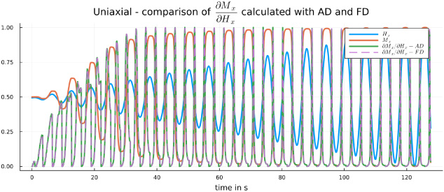
AD computed derivatives compared to Finite Difference results. Depicted on the plot are the excitation field H_x (blue line), the magnetization M_x (red line) resulting from evaluating the hysteresis model for the given excitation field and the computed derivatives (green and purple lines). All values are scaled to the range [0,1] for a better visibility.

Fig. 2.

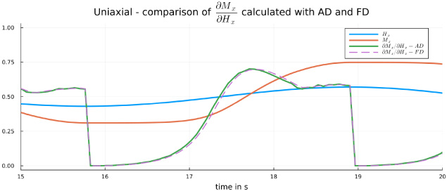
Zoomed view of Fig. 1 between 15 s and 20 s.

3. Parameter identification

3.1. Problem setup

As previously introduced, the hysteresis model parameters are the pinning forces 𝜒_i and the weights ω_i, with i = 1, 2, …, N and N the number of pseudo particles of the hysteresis model. We can concatenate these into one parameter vector $\begin{eqnarray}\mathbf{p}=[{\chi}_{1},{\chi}_{2},\ldots ,{\chi}_{\text{N}},{\omega}_{1},{\omega}_{2},\ldots ,{\omega}_{\text{N}}]^{T}=[\boldsymbol{\boldsymbol{\it\chi}},\boldsymbol{\boldsymbol{\it\omega}}]^{T}.\end{eqnarray}$ (8) To simplify the notation as we are only dealing with uniaxial data, H = H (t) represents a scalar value of the H-field in the x-direction at a given time step t and H all of the H-field values concatenated into one vector of values $\begin{eqnarray}\mathbf{H}=[H(t_{0}),H(t_{1}),\ldots ,H(t_{N_{m}})]^{T},\end{eqnarray}$ (9) where N_m is the number of time steps or measurement points. The same is true for the magnetic induction B. Further we denote the hysteresis model function with $\hat{B}={\mathcal{H}}(H;\mathbf{p})$ and measurement data pairs (H_{m, i}, B_{m, i}), where i = 1, 2, . . . , N_m and the subscript m marks the values as measurements. In doing so we define the error measure between the measurements and the model output by $\begin{eqnarray}e(\mathbf{p})=\mathop{\sum }_{i=1}^{\text{N}_{\text{m}}}({\mathcal{H}}(H_{\text{m},i};\mathbf{p})-B_{\text{m},i})^{2}=\mathop{\sum }_{i=1}^{\text{N}_{\text{m}}}(\hat{B}_{i}-B_{\text{m},i})^{2}.\end{eqnarray}$ (10) Our goal is now to minimize this error with respect to the hysteresis model parameters p $\begin{eqnarray}\begin{array}{@{}ll@{}}p^{\ast }= & \displaystyle \mathop{\text{arg}∼\text{min}}_{\mathbf{p}=[\boldsymbol{\boldsymbol{\it\chi}},\boldsymbol{\boldsymbol{\it\omega}}]^{T}}e(\mathbf{p})\\[12.0pt] \text{s.t.}\quad & \displaystyle \mathop{\sum }_{i=1}^{\text{N}}{\omega}_{i}=1\\[12.0pt] & \begin{array}{@{}l@{}}{\omega}_{i}\geq 0\\[3.0pt] {\chi}_{i}\geq 0.\\ \end{array},\quad 1\leq i\leq \text{N}.\end{array}\end{eqnarray}$ (11) The hysteresis model parameters have constraints as given in (11). The sum of the weights needs to be equal to 1 and furthermore all of the weights and pinning forces need to be positive. This ensures the physical consistency and interpretability of the parameters in the context of the energy based hysteresis model.

It is evident that the number of hysteresis model parameters grows linearly with the number of pseudo particles. This becomes challenging to optimize as the number of parameters increases while also ensuring that the given parameter constraints are met. Therefore in the next section we go over a method of how to reduce the number of parameters and eliminate the need for a constrained optimization.

3.2. Parameter distribution functions

From [9,10] we see that it is possible to draw the hysteresis parameters ω from distributions like the gaussian or rayleigh distribution, Fig. 3. The pinning force 𝜒 is then chosen as the random variable and for each 𝜒_i we get a weight ω_i, depending on the used distribution function. For the normal (gaussian) distribution we can write this as $\begin{eqnarray}{\omega}_{i}={\mathcal{N}}({\chi}_{i};{\mu},{\sigma}^{2}).\end{eqnarray}$ (12) Where μ denotes the mean and σ ≥ 0 the standard deviation. More generally if we denote the distribution function with ${\mathcal{D}}_{f}$ and the distribution parameters as p_d then we can use a similar notation for any given distribution and even mixtures of distributions. Using this distribution function and its parameters we would write a normal distribution with parameters p_d = [μ, σ²] as $\begin{eqnarray}{\omega}_{i}={\mathcal{D}}_{f}({\chi}_{i};\mathbf{p}_{d}).\end{eqnarray}$ (13)

From (13) it is clear how one can calculate the weights given the pinning forces and the distribution parameters, but how do we choose the correct pinning force values? In [10] the pinning force values for a given distribution function and number of pseudo particles N are obtained as the optimal nodes for a piecewise constant approximation of the PDF (probability density function) of the given distribution. We adopt a similar approach where the error of a piecewise linear interpolation of the PDF is minimized by iteratively placing nodes in regions with the highest errors, as can be seen in Fig. 4. This iterative process is repeated until the number of nodes is equal to the number of pseudo particles N. The initial two points are chosen such that the first pinning force 𝜒₁ is 0 and the last one 𝜒_N is the maximal H-field value, which can be obtained from the underlying data. Therefore, for a given number of pseudo particles, maximal H-field value and distribution function with its parameters, the hysteresis model parameters 𝝌 and 𝝎 can be determined.

Fig. 3.

Shapes of the Gaussian, Rayleigh and Gumbel distribution. For more information about the distributions, see [11].

Fig. 4.

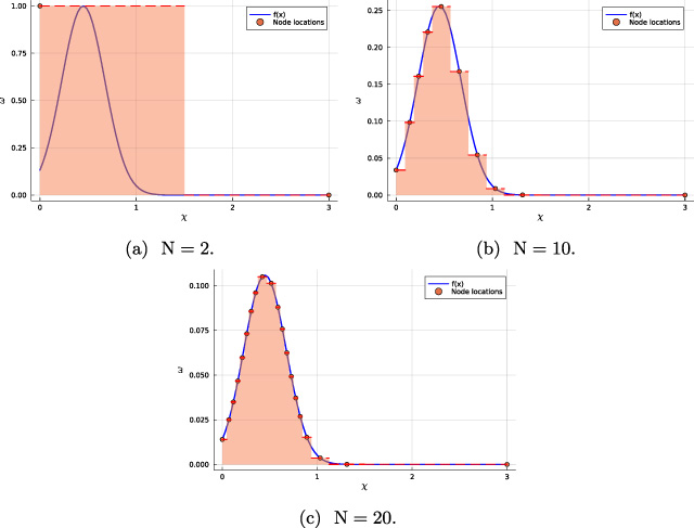
Hysteresis parameters drawn from a Gaussian distribution for different numbers of pseudo particles.

Further, we define a modified hysteresis model function ${\mathcal{H}}_{d}(H;\mathbf{p}_{d})$ which takes the distribution parameters p_d, generates the hysteresis model parameters p and finally calls the hysteresis model function ${\mathcal{H}}(H;\mathbf{p})$ . If we now reformulate the optimization problem from (11) to an optimization of the distribution function parameters p_d we get $\begin{eqnarray}\mathbf{p}_{d}^{\ast }=\mathop{\text{arg}∼\text{min}}_{\mathbf{p}_{d}}e_{d}(\mathbf{p}_{d})=\mathop{\text{arg}∼\text{min}}_{\mathbf{p}_{d}}\mathop{\sum }_{i=1}^{\text{N}_{\text{m}}}({\mathcal{H}}_{d}(H_{\text{m},i};\mathbf{p}_{d})-B_{\text{m},i})^{2}.\end{eqnarray}$ (14) If we compare the optimization problem from (11) and (14) we can see that the new optimization problem reduces the previous one down to an unconstrained optimization problem. Additionally, the number of optimization parameters is reduced significantly as it no longer depends on the number of pseudo particles. Further, using such a parametrization instead of directly prescribing the hysteresis model parameters p = [𝝌, 𝝎], we end up with a useful interface for sampling the hysteresis model with different parameter combinations.

3.3. Direct parameter identification

Here we solve the optimization problem given in ((14)) by optimizing the distribution parameters p_d while evaluating the hysteresis model directly and computing its derivatives with automatic differentiation. We showcase the performance on three synthetic cases, which were all generated with the gumbel distribution. The B-max-error measure is calculated as $\frac{\mathit{RMSE}}{B\text{-max}}\cdot 100\%$ , where B-max is obtained from the data. For the optimization a stochastic optimizer is used to do the initial global search and then the result is refined by a gradient based algorithm. In particular, for the global search we used the PSO algorithm [12] and for the local the BFGS algorithm [13]. There is no particular reason for choosing exactly these algorithms and one might have got comparable results even with different optimization methods. It was not the goal of the paper to investigate possible advantages of other optimizers as the obtained results with these were already sufficient. The same starting point is taken for all of the performed experiments. Further, the number of pseudo particles for the hysteresis model is 30 for each experiment. The obtained results are shown in Table 1.

Table 1
Distribution parameter p_d identification from synthetic data

Experiment True parameters Identified parameters RMSE B-max-error

1 [1350, 800] [1350.0, 800.0] 7.4951e-8 4.99e-6%

2 [3700, 1100] [3784.2, 1061.3] 7.1543e-3 0.4%

3 [6300, 420] [6283.3, 441.2] 1.8423e-1 0.12%

Experiment	True parameters	Identified parameters	RMSE	B-max-error
1	[1350, 800]	[1350.0, 800.0]	7.4951e-8	4.99e-6%
2	[3700, 1100]	[3784.2, 1061.3]	7.1543e-3	0.4%
3	[6300, 420]	[6283.3, 441.2]	1.8423e-1	0.12%

If on the other hand we solve the optimization problem from (11) we obtain the results in Table 2. The resulting hysteresis curves of these two approaches can also be seen in Fig. 5. The problem with the optimization in the space of hysteresis parameters p is that one has to deal with a large number of optimization parameters. Therefore, the optimization with the modified parametrization as in (14) leads to much better results. Applying the method on measurement data, we obtain a very good fitting model with a relative error of 0.14% from B-max. The resulting hysteresis curve is depicted in Fig. 6. One beneficial point which comes from the distribution function parametrization is that the number of pseudo particles can be easily adjusted and does not have a large influence on the accuracy if the distribution function parameters are correct. Therefore one can select a lower number of pseudo particles when performing the optimization and then after obtaining the correct parameters p_d = [μ, σ²] it is possible to adjust the number of pseudo particles.

Table 2

Hysteresis parameter p identification with same starting point as for p_d identification

Experiment	RMSE	B-max-error
1	1.2678e-1	8.16%
2	5.7703e-2	3.53%
3	8.0269e-1	4.8%

Fig. 5.

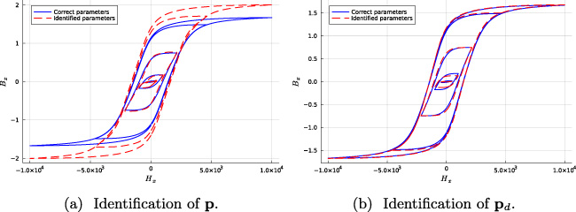
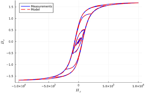
(a) Resulting hysteresis curves from parameters identified by finding the optimal p vector, (b) for finding the optimal p_d vector.

Fig. 6.

Measurement data compared to the model output with the identified parameters.

3.4. Data generation

The basic idea behind the identification of the hysteresis model parameters with a neural network is to condition a neural network on data pairs (B_i, p_{d, i}) so that for a given B-field vector the network gives the appropriate parameters p_d. In doing so, we first need to generate the data. This is done by sampling the hysteresis model function ${\mathcal{H}}_{d}(H^{m};\mathbf{p}_{d})$ . For the input magnetic field we take the magnetic field used in the measurements H_m and generate a set of distribution function parameters p_d and for each one of these the B-field vector B. As the H-field is the same for all of the parameter combinations it is not used in the training but would be useful in the case where one would generalize over different input signals but this is out of the scope of this work.

The following table gives an overview of the data generated for the network training purposes. It is important to note that the type of the distribution has a great impact on the expressivity of the parameters generated with it. Therefore we include also the mixture model data which combines two distributions and allows for more complex parameter sets to be generated. For each dataset N_s samples were generated with a latin hypercube sampling plan as given in Table 3. From the 10000 generated samples 5% is used for testing purposes which is a total of 500 points. The hysteresis model parameters obtained, are rescaled depending on the maximum H-field. This way one can reuse the generated parameter sets even for different input signals but needs to recompute the B-field values given the parameters.

Table 3
Generated datasets for neural network training

Dataset Distribution Min Params Max Params N N _s

1 Gaussian [0, 1e-6] [0.8, 0.1] 30 10000

2 Gumbel [0, 1e-6] [0.8, 0.1] 30 10000

3 Mixture [0, 1e-6, 0, 1e-6] [0.8, 0.1, 0.8, 0.1] 30 10000

Dataset	Distribution	Min Params	Max Params	N	N _s
1	Gaussian	[0, 1e-6]	[0.8, 0.1]	30	10000
2	Gumbel	[0, 1e-6]	[0.8, 0.1]	30	10000
3	Mixture	[0, 1e-6, 0, 1e-6]	[0.8, 0.1, 0.8, 0.1]	30	10000

3.5. Neural networks for parameter identification

Now that we have defined the problem and obtained data for the neural network we can describe the basic idea of identifying the parameters of the hysteresis model via neural networks. We denote the neural network as a function f_NN(x; θ), where x is the neural network input and θ the neural network parameters. As we have the data pairs (B_i, p_{d, i}) we can simply condition the neural network to do the mapping from B-field values to the distribution parameters, as in (15) $\begin{eqnarray}\hat{\mathbf{p}}_{d,i}=f_{NN}(\mathbf{B}_{i};{\theta}^{\ast }).\end{eqnarray}$ (15) To obtain the optimal neural network parameters θ^∗ we need to solve an optimization problem involving the neural network parameters. This is done by defining a loss function ${\mathcal{L}}(\mathbf{x};{\theta})$ (16) which is then minimized as in (17) $\begin{eqnarray}\displaystyle {\mathcal{L}}(\mathbf{B},\mathbf{p};{\theta}) & = & \displaystyle \frac{1}{N_{s}}\mathop{\sum }_{i=1}^{N_{s}}(f_{NN}(\mathbf{B}_{i};{\theta})-\mathbf{p}_{i})^{2}\end{eqnarray}$ (16) $\begin{eqnarray}\displaystyle {\theta}^{\ast } & = & \displaystyle \mathop{\text{arg}∼\text{min}}_{{\theta}}{\mathcal{L}}(\mathbf{B},\mathbf{p};{\theta}).\end{eqnarray}$ (17) For the training process we took 500 B-field values from each dataset entry so that the size of the network was manageable. The network itself is a simple fully connected network with the layer configuration given as [500, 32, 32, 32, 1]. The first layer of the network has 500 neurons to accommodate the 500 B-field values as inputs. We have chosen in this case 3 hidden layers each with 32 neurons to keep the model as simple as possible but able to fit the given data. One network was trained for each distribution parameter which improves the performance significantly over the case where one network approximates all at once. Even though it would seem to be a bit more practical to have only one network approximate all distribution parameters, this actually makes the whole problem much harder. First, the network needs to fit two values which represent two completely different properties and which have no correlation with each other. Secondly, to make this work one would require a much more expressive network, more layers and neurons. For these reasons it is much easier to just use two small separate networks to solve the problem. The loss convergence can be seen in Fig. 7. For the sake of completeness we also evaluate the models on the previously used data points as in Table 1. As we can see in Table 4 and Table 5, model 2 outperforms the other models. This is not a surprise given the fact that the points were generated using the gumbel function, same as the training data for model 2. The main goal of these models is to be useful for parameter identification on measurement data for which we do not know the underlying distribution function, which describes the hysteresis parameters. Therefore we can use the pretrained networks and instantly get predictions of the parameters for different distributions, which the models represent. Out of these we can pick the parameters which minimize the error for the given measurements. Therefore the actual performance metric for these is to test them on measurement data as shown in Fig. 6. Doing so for the three different models we obtain the results given in Table 6. The hysteresis curve corresponding to the model 2 with the smallest error is shown in Fig. 8. Although small, the main cost of this approach comes from the optimization process of the neural network parameters and the sampling of the hysteresis model. The benefit lies in the fact that the trained network and the present datasets can be utilized for the parameter identification of other materials given the same excitation field was used for the measurements as in the dataset generation. From the results it is obvious that the direct parameter identification procedure is outperforming the neural networks. Because of this one could also combine the neural network identification with the direct optimization procedure. This can be done by using the neural network to generate a starting point, which is not far away from the optimum. The direct optimization can then be applied with this starting point without the need for a stochastic global search method.

Fig. 7.

Loss convergence for the training of the network predicting the μ parameter of p_d over 2000 epochs. The loss on the training data is given in blue while the loss on the validation data, which the network doesn’t see while training, is shown in orange. The loss curves of the networks predicting the other parameters are very similar to this one and are therefore left out.

Table 4

Root mean square errors of the three neural networks (M1, M2, M3) when comparing the hysteresis curves obtained from the predicted parameters

Experiment	RMSE-M1	RMSE-M2	RMSE-M3
1	14.5535e-3	2.9966e-3	70.5231e-3
2	13.8293e-3	2.8950e-3	53.0703e-3
3	2.9323e-3	8.2015e-4	31.0362e-3

Table 5

B-max-errors of the three neural networks (M1, M2, M3) when comparing the hysteresis curves obtained from the predicted parameters

Experiment	B_max-error-M1	B_max-error-M2	B_max-error-M3
1	0.87%	0.18%	4.22%
2	0.85%	0.17%	3.24%
3	0.18%	0.05%	1.99%

Table 6

Errors corresponding to the hysteresis curves calculated with the parameters obtained from the three constructed neural network models

Model	RMSE	B_max-error
1	45.6099e-3	2.72%
2	42.1761e-3	2.51%
3	241.4318e-3	14.38%

Fig. 8.

Measurement data compared to the model output with the identified parameters.

4. Conclusion

In this paper we have shown two approaches for identifying the parameters of an energy based hysteresis model. They make use of the automatically differentiable and computationally efficient implementation of the energy based hysteresis model in the Julia programming language. Furthermore a modified parametrization of the hysteresis model based on distribution functions is utilized which makes it possible to treat the identification process as an unconstrained optimization problem. This is then used in the first approach to identify the distribution function parameters which generate the full hysteresis parameter vector. This approach shows good performance on the synthetical test data and measurements. The previously mentioned problem with the starting point for the identification process can be partially alleviated by running a stochastic optimizer first and then using its endpoint as the starting point for the BFGS algorithm. This way the global search is performed with the stochastic method and the local with the deterministic one. In the second approach a neural network, which is conditioned on synthetic data, is used to predict the parameters of the distribution functions given the B-field values. This method also gives good results for both, the synthetic test cases and the measurement values. One important point here is the data generation part. Care needs to be taken so that the generated dataset covers a large space of possible solutions from which the network can learn. This needs to be investigated further to find efficient ways of setting up the sampling. Other outlook points for this work include the application to measurements from a rotational single sheet tester and more complex excitation field signals.

Footnotes

Acknowledgement

The work is supported by the joint DFG/FWF Collaborative Research Center CREATOR (CRC - TRR361/F90) at TU Darmstadt, TU Graz and JKU Linz.

References

Neto

F.D.M.

and da Silva Neto

A.J.

, An Introduction to Inverse Problems with Applications, Berlin Heidelberg, 2013, doi:10.1007/978-3-642-32557-1.

Bergqvist

, Magnetic vector hysteresis model with dry friction-like pinning, Physica B: Condensed Matter233(4) (1997), 342–347, doi:10.1016/S0921-4526(97)00319-0.

Baydin

A.G.

Pearlmutter

B.A.

and Radul

A.A.

, Automatic differentiation in machine learning: a survey, JMLR.org18(1) (2017), 5595–5637.

Sablik

and Jiles

, Coupled magnetoelastic theory of magnetic and magnetostrictive hysteresis, IEEE Transactions on Magnetics29 (1993), 2113–2123.

Prigozhin

Sokolovsky

Barrett

J.W.

and Zirka

S.E.

, On the energy-based variational model for vector magnetic hysteresis, IEEE Transactions on Magnetics52(12) (2016), 1–11, doi:10.1109/TMAG.2016.2599143.

Revels

Lubin

and Papamarkou

, Forward-mode automatic differentiation in Julia 2021, Astrophysics Source Code Library, record ascl:2102.015.

Kelley

C.T.

, ReverseDiff.jl. https://github.com/JuliaDiff/ReverseDiff.jl. Julia Package. 2020.

Innes

, Don’t unroll adjoint: Differentiating ssa-form programs, CoRR (2018), arXiv:abs/1810.07951.

Tolentino

G.C.A.

Leite

J.V.

Rossi

Ninet

Parent

and Blaszkowski

, Modeling of magnetic anisotropy in electrical steel sheet by means of cumulative distribution functions of gaussians, IEEE Transactions on Magnetics58 (2022), 1–5.

10.

Jacques

, Energy-based magnetic hysteresis models - theoretical development and finite element formulations, PhD thesis, ULiège - Université de Liège, 21 November 2018.

11.

Lin

White

J.M.

Byrne

, Distributions.jl: Definition and modeling of probability distributions in the JuliaStats ecosystem, Journal of Statistical Software 98 (2021), doi:10.18637/jss.v098.i16.

12.

Juneja

and Nagar

S.K.

, Particle swarm optimization algorithm and its parameters: A review, in: 2016 International Conference on Control, Computing, Communication and Materials (ICCCCM), IEEE, Allahbad, India, 2016.

13.

Fletcher

, Practical Methods of Optimization, John Wiley and Sons, Ltd, 2000.