3D analytical magnetic model calculation for Halbach PM induction heater planar topology

Abstract

In this work, a 3D analytical magnetic model based on hybridation of the sub-domain’s method and the image’s theory to compute magnetic field and translational motion eddy current in the conducting plate of the Halbach permanent magnet induction heater planar topology is developed. The main objective is to remedy the problem of the transverse edge effect, and hence improving the efficiency of analytical model and the accuracy of results. The developed model also allows fast and precise simulations of 3D magnetic phenomena, and presents an important reduction in computation time compared to 3D finite element simulations.

Keywords

Eddy currents 3D analytical solution permanent magnet induction heating transverse edge effect Halbach arrangement

1. Introduction

The end effect is present in any electromagnetic device; in cylindrical structures, this effect is mainly present along the axial length. It is no longer the same in planar topology where end effects are present, in two directions, especially the finite width effect or edge effect, due to the closing of the currents inside the active part of the armature. Therefore taking into account the 3D aspects in the development of models for the magnetic field distribution in these topologies is desirable [1–3] because the planar machines have non-negligible edge effects which can induce high level errors in some cases depending on the application [4–8].

The studied geometry in Fig. 1, presents important magnetic end effects that deserve to be taken into consideration in the modelling approach of this type of induction heater composed of two permanent magnets (PM) inductors with quasi Halbach magnetization arrangement. The heating conducting plate subjected to a linear oscillatory motion (V_max = 0.5 to 1.2 m/s) is placed between these two inductors. The motion creates induced currents which dissipate a heating power by Joule effect [9,10].

In this paper, the developed 3D model will be particularly focused on the transverse end effect.

Then, in order to achieve the above-mentioned goal, a strongly 3D analytical model is developed and presented in this paper. First, a 3D magnetostatic field analytical solution of the magnetic scalar potential formulation is derived thanks to the separation of variables technique [7]. This helps to determine the 3D magnetic field distribution in the studied domain. Then, the motional eddy currents induced in the conductive workpiece are computed using the magnetic field strength formulation considering the finite transverse edge effects using the image’s method. The hybrid developed model takes into account the reaction magnetic field. The resulting heating power density in the moving conductive workpiece is calculated using two techniques without the need of any correction factor.

Finally, in order to validate the 3D developed model, the performances of a planar permanent magnet induction-heating device PMIHD (Fig. 1) are calculated. All results issued from the developed 3D analytical model agree well with those obtained by 3D finite element method (3D FEM).

Fig. 1.

Planar induction heater geometry with Halbach permanent magnets.

Fig. 2.

3D study geometric model.

2. Analysis of the 3D magnetic field model

First, the considered study domain is composed of three regions: air, iron and permanent magnets (Fig. 2). In this section, it is assumed that the conductive parts have no effect on the magnetic field. In other words, the magnetic reaction of the currents induced in the plate is not taken into account in this section. The assumption of considering the permeability of permanent magnets identical to that of air is close to reality if Neodymium-Iron-Boron (NdFeB, 𝜇_r = 1.05) type magnets are used. In the iron parts, an infinite relative magnetic permeability is considered. y = 0 is the plane of symmetry in Fig. 2.

Under the assumptions mentioned above, the magnetic field distribution is governed by the magnetic scalar potential formulation (Laplace and Poisson equations) which can be expressed in the different regions by the following equations: $\begin{eqnarray}\left\{\begin{array}{@{}ll@{}}\displaystyle \overrightarrow{{\nabla}}\cdot \overrightarrow{{\nabla}}U_{\text{I}}=\frac{1}{{\mu}_{r}}\overrightarrow{{\nabla}}\cdot \overrightarrow{M},\quad & \text{in region I}\\[11.0pt] \overrightarrow{{\nabla}}\cdot \overrightarrow{{\nabla}}U_{\text{II}}=0\quad & \text{in region II}\end{array}\right.\end{eqnarray}$ (1) where $\overrightarrow{M}$ is the magnetization vector of the magnets which have two components in the tangential (x) and normal (y) directions: $\begin{eqnarray}\overrightarrow{M}=M_{x}(x,z)\overrightarrow{u}_{x}+M_{y}(x,z)\overrightarrow{u}_{y}\end{eqnarray}$ (2) The magnetization vector is considered constant in the y direction and then its components depend on x and z coordinates. Considering the proposed arrangement of PMs in Fig. 1, Fig. 3 illustrates the distribution of the magnetization components M_x and M_y along the x-direction.

Fig. 3.

Magnetization (M_y) and (M_x) as a function of x.

In order to take into account the transverse edge effect, the main idea is to make the magnetization periodic in the z-direction with a spatial period of length 2D_z as it is illustrated in Fig. 4 for the PM dimensions and the corresponding M_y component distribution along the z-direction.

Fig. 4.

Magnetization component M_y as a function of z.

Based on the illustrated curves in Fig. 3 and Fig. 4, the magnetization is decomposed into double Fourier series along x- and z-directions leading to the following expressions for the magnetization components: $\begin{eqnarray}M_{x}(x,z)=\mathop{\sum }_{n=1}^{\infty }\mathop{\sum }_{m=1}^{\infty }M_{x,nm}\cos (W_{n}x)\cos (W_{m}z)\end{eqnarray}$ (3) where $\begin{eqnarray}\displaystyle M_{x,nm} & = & \displaystyle \frac{16B_{r}}{{\mu}_{0}nm{\pi}^{2}}\sin (W_{n}L_{ax})\sin (W_{m}L_{az})\nonumber\\ \displaystyle M_{y}(x,z) & = & \displaystyle \mathop{\sum }_{n=1}^{\infty }\mathop{\sum }_{m=1}^{\infty }M_{y,nm}\sin (W_{n}x)\cos (W_{m}z)\nonumber\end{eqnarray}$ where $\begin{eqnarray}M_{y,nm}=\frac{16B_{r}}{{\mu}_{0}nm{\pi}^{2}}\sin \left(\frac{W_{n}b}{2}\right)\sin \left(\frac{n{\pi}}{2}\right)\cos (W_{m}L_{az})\end{eqnarray}$ (4) with: $\begin{eqnarray}\left\{\begin{array}{@{}l@{}}\displaystyle W_{n}=\frac{n{\pi}}{{\tau}_{p}}\quad \\[15.60004pt] \displaystyle W_{m}=\frac{m{\pi}}{2D_{z}}\quad \end{array}\right.,\qquad \left\{\begin{array}{@{}l@{}}L_{ax}=a/2\quad \\ L_{az}=c/2\quad \\ D_{z}=2L_{az}\quad \\ {\tau}_{p}=(a+b+2e_{g})\quad \end{array}\right.\end{eqnarray}$ Notice that n and m are odd integers and B_r is the residual flux density of the permanent magnets.

2.1. Analytical solution of the 3D magnetostatic problem

The magnetic scalar potential in the region of the magnets (I) and the region of the air gap (II) are the solution of the Poisson and Laplace equations respectively. In Cartesian coordinates, using the method of separation of variables, the general solutions of the magnetic scalar potential U_I and U_II, are given as follows [7]: $\begin{eqnarray} \displaystyle U_{\text{I}}(x,y,z) & = & \displaystyle \Re\left[\mathop{\sum }_{n=1}^{\infty }\mathop{\sum }_{m=1}^{\infty }\left(A_{1\cdot nm}e^{ky}+B_{1,nm}e^{-ky}-\frac{jw_{n}M_{x,nm}}{k^{2}}\right)\times e^{j(W_{n}x)}\times \cos (W_{m}z)\right]\nonumber\\ \displaystyle U_{\text{II}}(x,y,z) & = & \displaystyle \Re\left[\mathop{\sum }_{n=1}^{\infty }\mathop{\sum }_{m=1}^{\infty }(A_{2\cdot nm}e^{ky}+B_{2,nm}e^{-ky})\times e^{j(W_{n}x)}\times \cos (W_{m}z)\right] \end{eqnarray}$ (5) with: $\begin{eqnarray}k=\sqrt{({W_{m}}^{2}+{W_{n}}^{2})}\end{eqnarray}$ Equations (5) have 4 × n × m unknown coefficients (A_{1, nm}, B_{1, nm}, A_{2, nm} and B_{2, nm}) which are determined using the boundary conditions and interface. Flux densities are derived from (5) thanks to the constitutive laws in each region: $\begin{eqnarray}\left\{\begin{array}{@{}ll@{}}\overrightarrow{B}_{\text{I}}={\mu}_{0}\overrightarrow{H}_{\text{I}}+\overrightarrow{B}_{r}=-{\mu}_{0}\overrightarrow{\text{grad}}∼U_{\text{I}}+\overrightarrow{B}_{r}\quad & \text{in region I}\\[4.0pt] \overrightarrow{B}_{\text{II}}={\mu}_{0}\overrightarrow{H}_{\text{II}}=-{\mu}_{0}\overrightarrow{\text{grad}}∼U_{\text{II}}\quad & \text{in region II}.\end{array}\right.\end{eqnarray}$

2.2. Eddy current coupling with Halbach magnets

The heated conductive plate is placed inside a double permanent magnet inductor and is subjected to a linear movement as it is illustrated in Fig. 1. The displacement of the workpiece in the static magnetic field generates induced currents that produce the necessary heating power [9].

Considering the geometry of Fig. 2 issued from symmetry consideration, it can be divided into three regions to solve the magnetostatic problem: magnets region (I), the air-gap region (II) and the conducting plate region (III) as it is shown in Fig. 3. The permeability of the iron yoke is assumed to be infinite and the corresponding region is not considered.

In the moving conductive plate (region III), only the time-invariant steady state is considered and the magnetic field satisfies the static approximation of the Maxwell equations: $\begin{eqnarray}\left\{\begin{array}{@{}l@{}}{\nabla}\cdot B_{\text{III}}=0\quad \\ \displaystyle {\nabla}\times H_{\text{III}}=J_{\text{III}}\quad \\[6.0pt] \displaystyle {\nabla}\times E_{\text{III}}=\frac{-\partial B_{\text{III}}}{-\partial t}=0\quad \end{array}\right.\end{eqnarray}$ (6) where E _III is the electric-field strength and J _III is the induced current density in region III. The Ohm’s law for moving conductor with reference to the stationary frame, which is fixed to the magnets, is given by: $\begin{eqnarray}J_{\text{III}}={\sigma}(E_{\text{III}}+(V\times B_{\text{III}})).\end{eqnarray}$ (7) From (6) and (7), the eddy-current problem in region III is reduced to a magnetostatic problem, which can be solved using an H-formulation as $\begin{eqnarray}{\nabla}^{2}H_{\text{III}}=-{\sigma}{\mu}_{0}{\nabla}\times (V\times H_{\text{III}})\end{eqnarray}$ (8) where 𝜎 is the conductivity and V = V_x is the velocity of the conducting plate parallel to the x-direction.

In a Cartesian coordinate system, the development of Poisson equation (8) can be governed by three partial derivative equations (PDEs): $\begin{eqnarray}\left\{\begin{array}{@{}l@{}}\displaystyle \frac{\partial ^{2}H_{\text{III}x}}{\partial ^{2}x}+\frac{\partial ^{2}H_{\text{III}x}}{\partial ^{2}y}+\frac{\partial ^{2}H_{\text{III}x}}{\partial ^{2}z}={\sigma}{\mu}_{0}v_{x}\frac{\partial H_{\text{III}x}}{\partial x}\quad \\[9.0pt] \displaystyle \frac{\partial ^{2}H_{\text{III}y}}{\partial ^{2}x}+\frac{\partial ^{2}H_{\text{III}y}}{\partial ^{2}y}+\frac{\partial ^{2}H_{\text{III}y}}{\partial ^{2}z}={\sigma}{\mu}_{0}v_{x}\frac{\partial H_{\text{III}y}}{\partial x}\quad \\[9.0pt] \displaystyle \frac{\partial ^{2}H_{\text{III}z}}{\partial ^{2}x}+\frac{\partial ^{2}H_{\text{III}z}}{\partial ^{2}y}+\frac{\partial ^{2}H_{\text{III}z}}{\partial ^{2}z}={\sigma}{\mu}_{0}v_{x}\frac{\partial H_{\text{III}z}}{\partial x}\quad \end{array}\right.\end{eqnarray}$ (9) By solving (9) and (1) subject to the magnetization components distributions given in (3) and (4), the expressions of the magnetic field strength components in region III, are given by Fourier expansions as follows: $\begin{eqnarray} \left\{ \begin{array}{@{} l@{}}\displaystyle H_{iiii,x}(x,y,z)=\Re\left[\mathop{\sum }_{n=1}^{\infty }\mathop{\sum }_{m=1}^{\infty }(A_{x3,nm}e^{{\lambda}y}+B_{x3,nm}e^{-{\lambda}y})\times e^{jW_{n}x}\times \cos (W_{m}z)\right]\quad \\ [14.39996pt] \displaystyle H_{\text{III},z}(x,y,z)=\Re\left[\mathop{\sum }_{n=1}^{\infty }\mathop{\sum }_{m=1}^{\infty }(A_{z3,nm}e^{{\lambda}y}+B_{z3,nm}e^{-{\lambda}y})\times e^{jW_{n}x}\times \cos (W_{m}z)\right]\quad \\ [14.39996pt] \displaystyle H_{\text{III},y}(x,y,z)=\Re\left[ \begin{array}{@{} l@{}}\displaystyle \mathop{\sum }_{n=1}^{\infty }\mathop{\sum }_{m=1}^{\infty }\frac{-1}{W_{m}}[jW_{n}(A_{z3,nm}e^{{\lambda}y}+B_{z3,nm}e^{-{\lambda}y})-{\lambda}(A_{x3,nm}e^{{\lambda}y}-B_{x3,nm}e^{-{\lambda}y})]\\ [14.39996pt] \quad \times ∼e^{jW_{n}x}\times \sin (W_{m}z) \end{array} \right]\quad \end{array} \right. \end{eqnarray}$ (10) with: $\begin{eqnarray}{\lambda}=\sqrt{({W_{m}}^{2}+{W_{n}}^{2}+j{\sigma}{\mu}_{0}v_{x}W_{n})}.\end{eqnarray}$ One can note that the periodic boundary conditions in x- and z-directions explained above (Figs 3 and 4) are incorporated in the magnetic field strength expressions given above (10). The remaining boundary conditions between the regions of Fig. 5 can be exploited as follows:

In y = 0 and y = y₃ = p + e + d $\begin{eqnarray}\left\{\begin{array}{@{}l@{}}U_{\text{I}}(x,y_{3},z)=0\quad \\[2.39996pt] H_{\text{III},x}(x,0,z)=0\quad \\[4.79993pt] \displaystyle \frac{\partial H_{\text{III}y}(x,0,z)}{\partial y}=0\quad \end{array}\right.\end{eqnarray}$ (11)

In y = y₂ = p + e $\begin{eqnarray}\left\{\begin{array}{@{}l@{}}U_{\text{I}}(x,y_{2},z)=U_{\text{II}}(x,y_{2},z)\quad \\[4.79993pt] \displaystyle \frac{\partial \text{U}_{\text{I}}(x,y_{2},z)}{\partial y}=\frac{\partial \text{U}_{\text{II}}(x,y_{2},z)}{\partial y}-M_{z}(x,z)\quad \end{array}\right.\end{eqnarray}$ (12)

In y = y₁ = p $\begin{eqnarray}\left\{\begin{array}{@{}l@{}}\displaystyle \frac{\partial U_{\text{II}}(x,y_{1},z)}{\partial x}=-H_{\text{III},x}(x,y_{1},z)\quad \\[7.20007pt] \displaystyle \frac{\partial U_{\text{II}}(x,y_{1},z)}{\partial y}=-H_{\text{III},y}(x,y_{1},z)\quad \\[7.20007pt] \displaystyle \frac{\partial U_{\text{II}}(x,y_{1},z)}{\partial z}=-H_{\text{III},z}(x,y_{1},z)\quad \end{array}\right.\end{eqnarray}$ (13)

2.3. Eddy current, induced power and forces expressions

The eddy currents in the conducting workpiece are computed using Maxwell-Ampere law: $\begin{eqnarray}\overrightarrow{J}_{\text{III}}=\overrightarrow{{\nabla}}\wedge \overrightarrow{H}_{\text{III}}.\end{eqnarray}$ (14)

After calculation, the components of the induced current density in the conducting plate are given as follows: $\begin{eqnarray} \displaystyle J_{\text{III},x}(x,y,z) & = & \displaystyle \Re\left[ \begin{array}{@{} l@{}}\displaystyle \mathop{\sum }_{n=1}^{\infty }\mathop{\sum }_{m=1}^{\infty }\left[ \begin{array}{@{} l@{}}\displaystyle \left(\frac{W_{n}^{2}-{\lambda}^{2}}{W_{m}}(A_{z\text{III}}e^{{\lambda}y}+B_{z\text{III}}e^{-{\lambda}y})\right.\\ [11.0pt] \displaystyle \left.-\frac{j{\lambda}W_{n}}{W_{m}}(A_{x\text{III}}e^{{\lambda}y}-B_{x\text{III}}e^{{\lambda}y})\right)\times e^{jW_{n}x} \end{array} \right]\\ \quad \times ∼\sin (W_{m}z) \end{array} \right]\nonumber\\ \displaystyle J_{iii,z}(x,y,z) & = & \displaystyle \Re\left[ \begin{array}{@{} l@{}}\displaystyle \mathop{\sum }_{n=1}^{\infty }\mathop{\sum }_{m=1}^{\infty }\left[ \begin{array}{@{} l@{}}jW_{n}(A_{z\text{III}}e^{{\lambda}y}+B_{z\text{III}}e^{-{\lambda}y})\\ [2.39996pt] -{\lambda}(A_{x\text{III}}e^{{\lambda}y}-B_{x\text{III}}e^{{\lambda}y})\times e^{jW_{n}x} \end{array} \right]\\ \quad \times ∼\cos (W_{m}z) \end{array} \right]. \end{eqnarray}$ (15) Resulting power loss density using the 3D model is obtained as: $\begin{eqnarray}p(x,y,z)=\frac{1}{{\sigma}}((J_{\text{III},x}(x,y,z))^{2}+(J_{\text{III},z}(x,y,z))^{2}).\end{eqnarray}$ (16) The total heating power dissipated by Joule effect in the conducting plate is computed by the integration of the power loss density in the volume of the plate: $\begin{eqnarray}p_{T}=\int _{-L/2}^{L/2}\int _{-y_{1}}^{y_{1}}\int _{-z_{p}/2}^{z_{p}/2}\left(\frac{1}{{\sigma}}(J_{x}(x,y,z)^{2}+J_{z}(x,y,z)^{2})\right)dxdydz\end{eqnarray}$ (17) where z_p is the transversal length of the workpiece.

Fig. 5.

Regions of the studied geometry in the plane (x − y).

Using Laplace force expression, the electromagnetic braking force exerted on the workpiece can be given by: $\begin{eqnarray}\overrightarrow{F}=\iiint _{{\tau}}(\overrightarrow{J}\times \overrightarrow{B})dxdydz\end{eqnarray}$ (18) leading to the following scalar expression of the x-component of the force: $\begin{eqnarray}F_{x}=\int _{-L/2}^{L/2}\int _{-y_{1}}^{y_{1}}\int _{-z_{p}/2}^{z_{p}/2}B_{y\text{III}}(x,y,z)\times J_{z}(x,y,z)dxdydz.\end{eqnarray}$ (19)

In addition to its expression given in (17), the total heating power dissipated by Joule effect in the conducting workpiece can be calculated thanks to the exerted force x-component and the workpiece velocity by: $\begin{eqnarray}p_{T}=F_{x}\times V.\end{eqnarray}$ (20)

3. 3D finite-element analysis model

This section focuses on the presentation of the 3D finite element model using 3-D FEMs to verify the correctness of the 3D analytical solutions. The magnetic and electrical quantities with the dimensions listed in Table 1 are calculated . The nonlinear characteristic of iron is treated as a static field characteristic and can be analyzed ignoring hysteresis. The relative magnetic permeability considered is 𝜇_r = 4000.

The whole studied domain is shown in Fig. 6 where the mesh elements shape is tetrahedral and the mapping mesh is imposed. The numbers of (nodes, elements) are (360 140) leading to the resolution of a global algebraic system having 2287999 degrees of freedom.

Table 1
Physical and geometrical parameters of the studied induction heater

Symbol Quantity Value

2 ∗ y₁ Workpiece thickness 15 mm

e Air-gap thickness 3 mm

d Permanent magnets thickness 10 mm

z _a Permanent magnets length 80 mm

a Permanent magnets width 40 mm

b Permanent magnets width 40 mm

e _g Distance between two magnets 4 mm

z _p Width workpiece 80 mm

L Workpiece length 400 mm

y _c Iron yoke thickness 20 mm

z _c Iron yoke width 80 mm

V Speed of translation Variable m/s

Br Remanent flux density of magnet 1.2 T

𝜎 Electrical conductivity at T₀ 37 × 10⁶ (Ω⋅m)⁻¹

Symbol	Quantity	Value
2 ∗ y₁	Workpiece thickness	15 mm
e	Air-gap thickness	3 mm
d	Permanent magnets thickness	10 mm
z _a	Permanent magnets length	80 mm
a	Permanent magnets width	40 mm
b	Permanent magnets width	40 mm
e _g	Distance between two magnets	4 mm
z _p	Width workpiece	80 mm
L	Workpiece length	400 mm
y _c	Iron yoke thickness	20 mm
z _c	Iron yoke width	80 mm
V	Speed of translation	Variable m/s
Br	Remanent flux density of magnet	1.2 T
𝜎	Electrical conductivity at T₀	37 × 10⁶ (Ω⋅m)⁻¹

Fig. 6.

Finite element mesh of the whole studied domain.

4. Results and validation

In order to validate the 3D magnetic model developed previously, an application on an induction heater similar to the one proposed in [6] was carried out.

The physical properties and geometrical dimensions of the studied induction heater are shown in Table 1.

Fig. 7.

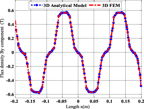
Flux density y-component B_y versus longitudinal coordinate x at (y = y₁) the surface of the workpiece and z = 0, (V = 0).

The distribution of the flux density component B_y along the longitudinal coordinate x at the surface of the workpiece (y = y₁) at z = 0 is illustrated in Fig. 7. One can remark that the B_y values obtained by 3D analytical model and 3D FEM simulation are in a good agreement. This component of the induction presents a periodic variation in this direction with amplitude of 0.58 T.

On the other hand, at z = z_p∕2, the flux density component B_y waveform versus the longitudinal coordinate x at y = y₁ and illustrated in Fig. 8 is obtained thanks to the 3D analytical model and is compared to the 3D FEM simulations. One can note that this component of the flux density presents a periodic variation in this direction, but its maximum value decreases considerably between the center plane at z = 0 (0.58 T) of the transversal workpiece extremities at z = ±z_p∕2 (0.28 T).

Fig. 8.

Flux density y-component B_y versus longitudinal coordinate x at (y = y₁ and z = z_p∕2), V = 0.

Fig. 9.

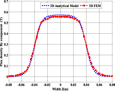
Flux density component B_y versus z-direction at y = 0 and x = (a + b)∕2 + e_g (North pole), V = 0.

Figure 9 illustrates the spatial distribution of the flux density component B_y versus the transversal coordinate z at x = (a + b)∕2 + e_g (under a North pole) for y = 0. One observe that the flux density component B_y remains approximately constant in the central region of the workpiece, collapses by 50% at its transversal ends and is totally cancelled at a distance equal to half the workpiece transversal length (z = z_p or − z_p) which validates the analytical model assumption concerning the B_y waveform in the z-direction.

Figures 10 and 11 illustrate respectively the evolution of the induced current density components J_z and J_x versus x-direction in the center of the workpiece, at z = 0 for J_z and z = z₁∕2 for J_x for a linear speed V_max = 0.5 m∕s. One can observe that these components present a periodic variation in this direction with amplitudes (J_z = 5.89 10⁶ A/m² and J_x = 6.10⁶ A/m²).

Figures 12 and 13 show respectively the distribution of the induced current component J_z along the coordinate z at the center (y = 0) of the workpiece for x = 0.044 m and the distribution of the induced current component J_x along the coordinate z at the center (y = 0) of the workpiece for x = 0.044 m.

Fig. 10.

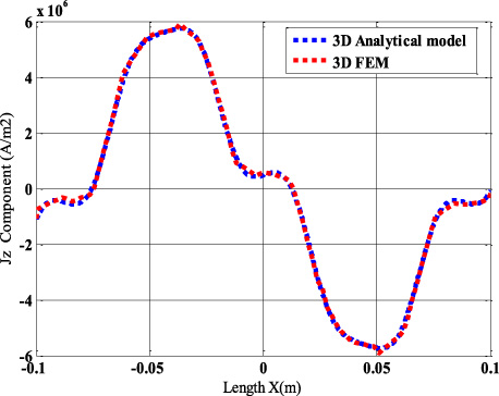
Induced current density component J_z in the middle of the conducting workpiece (y = y₁) versus the x coordinate (z = 0, V_x = 0.5 m/s).

Fig. 11.

Induced current density component J_x in the middle of the conducting work piece (y = y₁) versus the x coordinate (z = z_p∕2, V_x = 0.5 m/s).

Fig. 12.

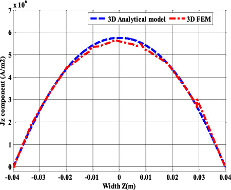
Induced current density component J_z in the middle of the conducting workpiece (y = 0) versus z coordinate (x = 0, V_x = 0.5 m/s).

Fig. 13.

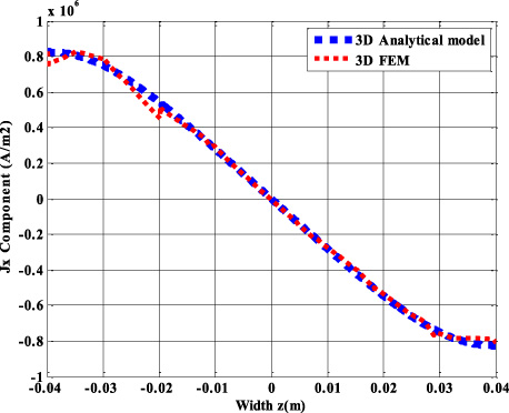
Induced current density component J_x in the middle of the conducting workpiece (y = 0) versus z coordinate (x = 0.044 m, V_x = 0.5 m/s).

Fig. 14.

Total induced heating power in the conducting workpiece versus velocity values (V).

Figure 14 illustrates the variation of the total heating power induced in the workpiece as a function of the speed, calculated by the 3D analytical and 3D numerical models. It is clearly shown that the developed 3D analytical model gives a better estimation of the heating power than the quasi-3D model developed earlier [6]. The results obtained by the 3D analytical model show very good agreement with those obtained by the 3D FEM.

Fig. 15.

Braking force F_x(N) in the conducting workpiece versus velocity values (V).

Comparing the 3D analytical results for the induced current density with the corresponding 3D FEM results especially in the extremity regions of the conductive workpiece, it appears clearly that the proposed analytical 3D model gives sufficiently accurate results.

Figure 15 shows the variation of the electromagnetic braking force F_x(N) in the workpiece as a function of the speed, calculated by the 3D analytical and 3D FEM models. It is clearly shown that the analytical model developed in 3D gives a better estimate of the braking force. After calculating the relative difference between the results obtained by the 3D analytical model and the 3D finite element model, the error is very low, around 0.6% at a translation speed lower than V = 0.8 m/s. This difference remains small when the speed increases (around 1% for V = 1 m/s). The comparison of the results obtained by the 3D analytical model with those given by showed very good agreement with respect to the results obtained by the 3D FEM.

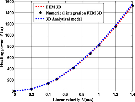
Figure 16 illustrates the variation of the total induced heating power in the conducting workpiece as a function of the speed, obtained by the different 3D analytical models using Eqs (17) and (20), and 3D FEM model by 3D numerical integration of equations (17) and (20). It can be seen that these results are in good agreement. After calculating the relative difference between the results obtained by the 3D analytical model and the 3D finite element model, we see that the error is very low, around 0.6% at a translation speed lower than V = 0.8 m/s. This difference remains small when the speed increases (around 1.4% for V = 1.2 m/s).

It clearly appears that 3D developed analytical model gives a very accurate estimate of the heating power and magnetic force. That proof the improvement of the models developed in [7] because, in this work, we took into consideration the transverse edge effect, the exact distribution of induced currents and the magnetic reaction of the armature.

Fig. 16.

Total induced heating power versus constant translation velocity.

Also, the proposed model presents an important reduction in computation time. Indeed, for a given velocity, the calculation time for the 3D FEM (3D mesh of 360 140 tetrahedral elements leading to the resolution of a global algebraic system having 2287999 degrees of freedom) using a workstation (4 GB of RAM, Intel® Core^TM processor i5-4258U) is about 178 s, while that time is about 0.34 s when using the analytical model. Note that, for all analytical calculations, we have considered a same number of harmonics in the x and y directions, n = 25 and m = 25. Finally, the proposed model can be used as an effective tool in a design optimization procedure of the induction heater and planar permanent magnet machines.

5. Conclusion

The new 3D electromagnetic analytical developed model, makes it possible to calculate the distribution of the magnetic field in 3D in the real geometry and takes into account the transverse edge effect (without approximation in 2D) and the reaction magnetic field, and consequently it makes it possible to calculate the exact values of the different overall quantities (induced currents, induced power, force). The developed model presents a very small computation time compared to the simulation by finite element method (3D FEM).

References

Diriye

Amara

and Barakat

, Three-dimensional modeling of permanents magnets synchronous machines using a 3D reluctance network, in: 2012 XXth International Conference on Electrical Machines, IEEE Explore, Alexandroupoli, Greece, 2018, pp. 2733–2738.

Pluk

K.J.W.

Jansen

J.W.

and Lomonova

E.A.

, 3-D hybrid analytical modeling: 3-D Fourier modeling combined with mesh-based 3-D magnetic equivalent circuits, IEEE Trans. Magn.51(12) (2015), 8208614.

Lubin

and Rezzoug

, 3-D analytical model for axial-flux eddy-current couplings and brakes under steady-state conditions, IEEE Trans. Magn.51(10) (2015), 8203712, 12 pages.

Paul

Wright

and Bird

J.Z.

, 3-D steady-state eddy current damping and stiffness for a finite thickenss conductive plate, IEEE Trans. Magn.50(11) (2014), 6301404.

Pluk

K.J.W.

van Beek

T.A.

Jansen

J.W.

and Lomonova

E.A.

, Modeling and measurements on a finite rectangular conducting plate in an eddy current damper, IEEE Trans. Industrial Electronics61(8) (2014), 4061–4072.

Abdi

Ouazir

Barakat

and Amara

, Transient quasi-3D magneto-thermal analytical solution in PM induction heating device, COMPEL - The International Journal for Computation and Mathematics in Electrical and Electronic Engineering39(5) (2020), 1131–1144.

Abdi

Ouazir

Barakat

and Amara

, 3D transient non-linear magneto-thermal analytical model calculation in PM induction heating device, Progress in Electromagnetics Research B95 (2022), 81–101.

Jin

Tian

Guo

Lei

and Zhu

, 3-D analytical magnetic field analysis of the eddy current coupling with halbach magnets, IEEE Transactions on Magnetics56(1) (2020), 1–4.

Abdi

Ouazir

Barakat

and Amara

, Permanent magnet linear induction heating device: newtopology enhancing performances, COMPEL37(5) (2018), 1755–1767.