Application of Multi-Column Heterogeneous Convolutional Neural Networks in image classification

Abstract

Image classification is an important research direction of computer vision. Convolutional neural network is a deep feedforward neural network model. It uses the deep learning idea and shows good performance in multiple image classification fields such as speech recognition, face recognition, motion analysis, and medical diagnosis. However, a single-structure convolutional neural network is prone to overfitting problems. The main reason for the overfitting problem is that the learning model overfits the training set and results in the lack of generalization performance, which affects the feature extraction and judgment of the test set.

This paper presents a structure model for Multi-Column Heterogeneous Convolutional Neural Networks. Multi-Column Heterogeneous Convolutional Neural Networks are used in image classification. We construct several convolutional neural networks with different structures by setting different size of convolution kernels and different number of feature maps. Image features are learned from multiple perspectives. Each convolutional neural network model is trained on the training set, and the different network models are fitted to the training set. Finally, through the sliding window, the output of each network is fused to obtain a relatively better prediction result. Experiments show that Multi-Column Heterogeneous Convolutional Neural Networks reduce the overfitting problem to a certain extent, and the accuracy of object recognition is improved compared to the single structure convolutional neural network.

Keywords

Image classification Multi-Column Heterogeneous Convolutional Neural Network convolutional neural network

1. Introduction

Computer vision is an important branch of artificial intelligence. Its goal is to make computers have the ability to perceive and understand image semantic information similar to humans [12]. Image classification is an important research direction of computer vision. It refers to the image processing method that distinguishes different types of targets by feature extraction of original images.

Early image classification tasks mainly focused on the design of image features. The extraction of features mainly focuses on features such as texture [13, 15], color [11], and shape of the image [16, 6], using classifiers such as decision tree [5], support vector machine (SVM) [14], and artificial neural network [7] to classify images. At the same time, many excellent feature matching algorithms have emerged, such as SIFT [2], SURF [8], and FAST [4], which all greatly improved the accuracy of image classification.

However, these artificially designed feature algorithms mainly rely on the designer’s experience and are designed for specific applications in a certain field. Once the application field changes, the accuracy of the features will decline, and the generalization ability was weak. On the other hand, artificial design features are generally based on underlying features such as colors, textures, etc. These underlying features do not express the high-level semantic information of the image well, so feature expression capabilities are limited.

Convolutional neural network (CNN) can automatically learn the underlying features of the image by supervised training and verification through large-scale labeled datasets, and through the forward propagation layer-by-layer to obtain high-level abstract features. CNN has a stronger feature learning ability and generalization than manual design features. CNN has greatly improved the accuracy of image classification, and even reached and exceeded the level of human beings. It has become the preferred method for image classification and has become a hot topic in the academic community.

In 1998, Lecun et al. [17] proposed the LeNet-5 convolutional neural network and optimized the network using local receptive fields and shared weights. The recognition error rate on the MNIST dataset was only 0.8%. LeNet-5 received extensive attention from the academic community.

In 2012, Alex et al. proposed AlexNet, a deep convolutional neural network model. Its network structure is deeper than LeNet-5. It consists of five layers of convolutional layers and uses ReLU activation function, Dropout, and Local Response Normalization (LRN), and uses two GPUs to speed up the training of the network model on the ImageNet dataset, which greatly accelerates the training speed of the network. Alexnet won the championship of ILSVRC2012 with absolute advantages, and laid the foundation for convolutional neural networks in the image classification field.

After AlexNet emerged a large number of excellent convolutional neural network models, such as the VGG network model proposed by Oxford University [10], Google’s GoogleNet [1], and deep residual network ResNet [9] proposed by Microsoft. These networks continue to refresh AlexNet’s records and have achieved increasingly higher accuracy in the image classification field.

In addition to research on the internal structure of the network, Ciresan et al. [3] proposed the Multi-Column Deep Neural Network (MCDNN), which used multiple networks to alleviate the overfitting problem of a single network and improved the generalization performance of the network. MCDNN uses multiple single convolutional neural networks with the same structure. Each convolutional neural network trains on the same training set. The difference is that each network performs different preprocessing before training that is, by randomly distorts the input image and adds noise to network training, thereby improving the generalization performance of the network model. The input images with different preprocessing have a more abundant expression, which helps the network to classify the image. Finally, the predicted values of the Multi-Column Deep Neural Network are averaged as the final output of the network model. Ciresan experimentally proved that Multi-column Deep Neural Network have achieved very good recognition effects on many object recognition datasets.

2. Multi-Column Heterogeneous Convolutional Neural Networks

Although Multi-Column Deep Neural Network has achieved better accuracy than traditional neural networks, there are two problems worth exploring.

First, in terms of the choice of network structure, Multi-Column Deep Neural Network adopts exactly the same convolutional neural network, which may limit the network learning different features. The advantage of multi-column networks over a single network is that different networks can learn image features from different perspectives. So through the changes in the network structure, increasing the differences between different networks is a potential way to improve the overall performance of the network.

Second, the method of fusing the prediction of the multi-column network by simply taking the mean is relatively simple. Because the classification ability of different networks is different, if the networks are fused with the same weight, not conducive to highlighting the best network for classification. Therefore, it is necessary to consider a more flexible network fusion mechanism.

2.1 Multi-Column Heterogeneous Convolutional Neural Networks

The convolution kernel plays an important role in the convolutional neural network operation process. It mainly affects the network model in two aspects. First, the size of the convolution kernel determines the scale of the receptive field, and also affects the size of feature map. Second, the number of convolution kernels affects the number of feature maps. In the field of image classification, there is no effective method to prove the size of the convolution kernel and the number of feature maps that achieve the best classification on a particular dataset.

This paper is inspired by Ciresan’s research, we use Multi-Columns Heterogeneous Convolutional Neural Networks (MCHCNN) for image classification. By setting different size of convolution kernels and different number of feature maps, construct convolutional neural networks with different structures, learn image features from multiple perspectives, and train all the convolutional neural networks on the training set. Making the different network fit the training set. Finally, through the sliding window, the output of each network is fused to obtain a relatively better prediction result.

A Multi-Column Heterogeneous Convolutional Neural Network is composed of a plurality of convolutional neural networks with different structures. A schematic diagram of the model is shown in Fig. 1.

Figure 1.

Multi-Column Heterogeneous Convolutional Neural Network.

2.2 Sliding window fusion mechanism

Ciresan et al. bring diversity of network models by performing different preprocessing on input images. Different from Ciresan’s idea, in a Multi-Column Heterogeneous Convolutional Neural Network, the diversity of the network comes from the structural differences of each convolutional neural network. For the same input image, each network will output an input-based prediction, and predictions from multiple networks need to be fused in an appropriate manner.

Some widely used classifier fusion methods include minimum rule, maximum rule, average rule, and product rule. The disadvantages of these traditional methods are that the functions are relatively simple and have certain applicability limitations. Therefore, we propose a classifier fusion method based on sliding window. Sliding window fusion is a generalized classifier fusion method. This method is more flexible and general than the traditional classifier fusion method. Experiments show that the sliding window fusion method can achieve better classifier fusion effect than the traditional single classifier fusion method.

Take the eight-column networks fusion process as an example. The flow of the sliding window fusion is shown in Fig. 2.

Figure 2.

Sliding window fusion process.

Based on an input image, operations are performed through columns of convolutional neural networks. Pre1 to Pre8 are the predicted probabilities for a certain class from the eight-column convolutional neural networks. These probabilities are first ordered from low to high. Then, a sliding window is applied to the sorted distribution to produce the final prediction.

The sliding window has two main tasks to complete: 1) Determine which network’s prediction results will eventually be used in the final fusion process. This function is determined by the sliding window’s starting point (Head) and the selection range (Range); 2) Determine the fusion method of the selected prediction result. This function is determined by the fusion parameter Operation. Because the sliding window area and the fusion method are all selectable, in the actual network fusion process, the sliding window fusion is more flexible than the traditional single fusion method.

Hyper-parameters in the sliding window (Head, Range, and Operation) can be obtained by training. The training method is to exhaust all parameter combinations on the training set and finally select the optimal parameters for testing. The complexity of training on the training set is O(n2), but the complexity of the testing process is reduced to O(1). In essence, the parameters of the sliding window fusion (Head, Range, and Operation) can be used as hyperparameters and manually set according to experience. Using the training method enables the entire system to get rid of artificial setting parameters, which is beneficial to improving the generality of the entire network.

3. Network design

In order to verify the effectiveness of Multi-Column Heterogeneous Convolutional Neural Networks, three representative datasets in image classification field were selected as experimental datasets, namely MNIST, CIFAR-10 and Caltech-256. The MNIST dataset is a hand-written character dataset. The images are all grayscale images with a total of 70,000 images. The image classes are 0 to 9 total ten handwritten fonts. There are 10 types of objects in the CIFAR-10 dataset, and the pictures are all RGB images; The Caltech-256 dataset has 256 objects, all RGB images. The difficulty of dataset recognition is gradually increasing, which is helpful to verify the validity and generalization ability of the proposed method.

3.1 Network for MNIST dataset

The MNIST hand-written character dataset consists of 60,000 training pictures and 10,000 test pictures, all of which are 32*32 grayscale pictures.

In the structure design of Multi-Column Heterogeneous Convolutional Neural Networks, a total of eight convolutional neural network models with different network structures were created in the experiment. The detailed information of these convolutional neural networks is shown in Table 1.

Table 1
Multi-Column Heterogeneous Convolutional Neural Network for MNIST

Network	Conv1	Conv2	Pooling	FC	Output
CNN1	16(3*3)	32(3*3)	2*2	128	10
CNN2	16(5*5)	32(3*3)	2*2	128	10
CNN3	16(7*7)	32(3*3)	2*2	128	10
CNN4	32(3*3)	64(3*3)	2*2	128	10
CNN5	32(5*5)	64(3*3)	2*2	128	10
CNN6	32(7*7)	64(3*3)	2*2	128	10

In Table 1, Conv1 and Conv2 represent convolutional layers, and Pooling represents a pooling layer. In the convolutional layer, m(n*n) indicates that the number of feature maps in this layer is m and the convolution kernel size is n*n. The pooling layer uses a convolution kernel size of 2*2, uses non-overlapping downsampling regions, and uses an average downsampling strategy. FC is a fully connected layer with a feature vector length of 128. Output is the output layer, which represents the judgment of the digital class. The activation function uses the most widely used RELU activation function.

The classification function uses the Softmax classifier. Softmax classifier calculates and returns the probability values of each class, and then selects the class with the largest predicted probability as the result. The formula for Softmax is as follows:

$\displaystyle h_{\theta}\left({x^{(i)}}\right)=\left[{{\begin{array}[]{c}{p% \left({y^{(i)}=1\left|{x^{(i)};\theta}\right.}\right)}\\ {p\left({y^{(i)}=2\left|{x^{(i)};\theta}\right.}\right)}\\ \vdots\\ {p\left({y^{(i)}=k\left|{x^{(i)};\theta}\right.}\right)}\\ \end{array}}}\right]=\frac{1}{\sum\limits_{j=1}^{k}{e^{\theta_{j}^{T}x^{(i)}}}% }\left[{{\begin{array}[]{c}{e^{\theta_{1}^{T}x^{(i)}}}\\ {e^{\theta_{2}^{T}x^{(i)}}}\\ \vdots\\ {e^{\theta_{k}^{T}x^{(i)}}}\\ \end{array}}}\right].$ (1)

The Softmax classifier has a total of n classes. It uses $\theta$ *x as the coefficient of the exponent e. There are n items in total. Then the Softmax classifier normalizes them and finally gets an n-dimensional column vector. Each column vector represents the probability value of the corresponding class.

The corresponding cost function with Softmax is:

$\displaystyle J\left(\theta\right)=-\frac{1}{m}\left[{\sum\limits_{i=1}^{m}{% \sum\limits_{j=1}^{k}{1\left\{{y^{(i)}=j}\right\}\log\frac{e^{\theta_{j}^{T}x^% {(i)}}}{\sum\limits_{l=1}^{k}{e^{\theta_{l}^{T}x^{(i)}}}}}}}\right]+\frac{% \lambda}{2}\sum\limits_{i=1}^{k}{\sum\limits_{j=0}^{n}{\theta_{ij}^{2}}}.$ (2)

The purpose of adding a weight attenuation term is to convert the cost function into a strictly convex function so that a unique solution can be guaranteed by solving the cost function.

3.2 Network for CIFAR-10 dataset

The CIFAR-10 dataset contains 60,000 32x32 color images in 10 different classes. The 10 different classes represent airplanes, cars, birds, cats, deer, dogs, frogs, horses, ships, and trucks. There are 6,000 images of each class. There are 50000 training images and 10000 test images.

In the design of Multi-Column Heterogeneous Convolutional Neural Networks, three convolutional neural network models with different structures are designed. In these network models, each network model has three convolutional layers, three pooling layers, two fully connected layers, and one output layer. The convolutional layer and the pooling layer are connected alternately, the fully connected layer is behind the last pooling layer, and the output layer is at the end. The number of feature maps and convolution kernel sizes are shown in Table 1. In Table 2, Conv1, Conv2, and Conv3 represent convolutional layers, and m(n*n) means that the number of feature maps in this layer is m, and the size of the convolution kernel is n*n. Pooling1, Pooling2, and Pooling3 represent the pooling layer, the convolution kernel is 2*2 with max-pooling. FC1 and FC2 are fully connected layers, and their feature vector length is 2048. Output is the output layer and represents the probability of the 10 objects.

Table 2
Multi-Column Heterogeneous Convolutional Neural Network for CIFAR-10

	CNN1	CNN2	CNN3
Conv1	64(5*5)	64(5*5)	64(3*3)
Pooling1	2*2	2*2	2*2
Conv2	128(5*5)	128(3*3)	128(3*3)
Pooling2	2*2	2*2	2*2
Conv3	256(5*5)	256(3*3)	256(3*3)
Pooling3	2*2	2*2	2*2
FC1	2048	2048	2048
FC2	2048	2048	2048
Output	10	10	10

The activation function uses Leaky Relu. This activation function is the same as the Relu activation function in the portion where the threshold is greater than zero, but in the portion less than zero is to multiply these thresholds by a very small value instead of zero. The formula for the Leaky Relu activation function is as follows:

$\displaystyle\mbox{y}_{i}=\left\{{{\begin{array}[]{*{20}c}{x_{i}}&{x_{i}% \geqslant 0}\\ {\alpha x_{i}}&{x_{i}<0}\\ \end{array}}}\right.$ (3)

The Leaky Relu activation function is used instead of Relu because Relu simply handled zero at the threshold less than zero. These less than zero neurons are in a state of inhibition and are called “dead spots”. These neurons cause the gradient to disappear. These neurons will no longer be activated and updated. This will result in the loss of information in the network, so it will also have a certain impact on the recognition effect.

3.3 Network for Caltech-256 dataset

Caltech-256 is an image object recognition dataset containing 30607 images, 256 object classes, and the number of images in each class is about 80 to 800. Caltech-256 has more classes and each class has relatively few training samples than CIFAR-10, so it has higher recognition difficulty.

The experiment uses the accurate model of OverFeat. The accurate model is more complex than the fast model, and has more feature maps and the number of convolutional layers. In the Caltech-256 dataset, the number of samples for each class is too small to training a CNN. This experiment adopts transfer learning to solve the problem of insufficient training samples. The OverFeat accurate model is trained on ImageNet, and the trained network is fine-tuned on the Caltech-256 dataset.

In order to improve the accuracy of the experiment, OverFeat’s accurate model is constructed into three different depths of CNN. OverFeat1 is a complete accurate model with a total of 24 layers. OverFeat2 consists of OverFeat’s first 22 layers; OverFeat3 consists of OverFeat’s first 20 layers. Layers 20, 22, and 24 happen to be the last three convolutional layers of OverFeat’s accurate model. For each convolutional neural network, a Softmax layer is added at the end of the network. During the transfer learning process, the training of network parameters is also limited to the Softmax layer.

4. Analysis of experimental results

4.1 Result for MNIST

The images used in the experiment were directly input into the constructed convolutional neural network models for training or testing without any preprocessing. All the convolutional neural networks with different structure completed 200 epochs training on the MNIST training set. For each trained network, tests were performed on MINIST test set. The results of the test are shown in Fig. 3.

From the experimental results, we can see that the performance of convolutional neural networks with different structures on the MNIST dataset is also different. The lowest error rate is CNN4, the error rate is only 0.69%; the highest error rate is CNN3, and the error rate is 1.44%. From these reluts we can see that the size of the convolution kernel and the number of feature maps have a great impact on the network performance. MCHCNN is the result of sliding window fusion. We can see that the result of sliding window fusion is lower than the best CNN4 error rate.

Experiments based on MNIST datasets have proved that Multi-Column Heterogeneous Convolutional Neural Networks achieve better object recognition performance than single-column convolutional neural networks after sliding window fusion.

Figure 3.

MNIST dataset experiment results.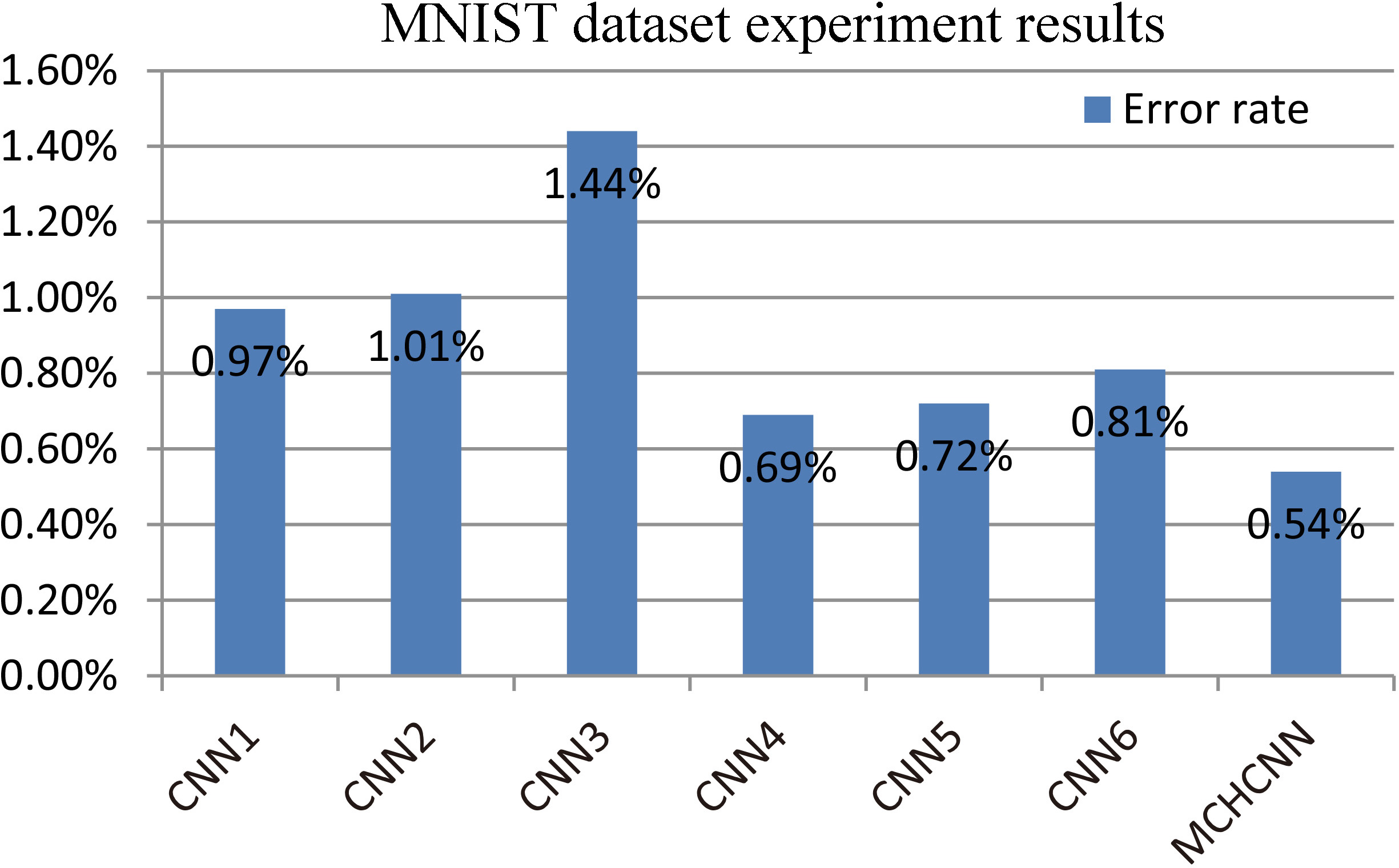

4.2 Result for CIFAR-10

All pictures in the dataset are normalized and whitened for global contrast. Then through the rotation of the image, more sample images are generated to augment the dataset. Each heterogeneous CNN was trained on the CIFAR-10 dataset, completing 2000 iterative training. All the trained networks fused their prediction probabilities for each class as the final prediction. The trained network is tested on the test set. The results of the final accuracy rate are shown in Fig. 4.

Figure 4.

CIFAR-10 dataset experiment results.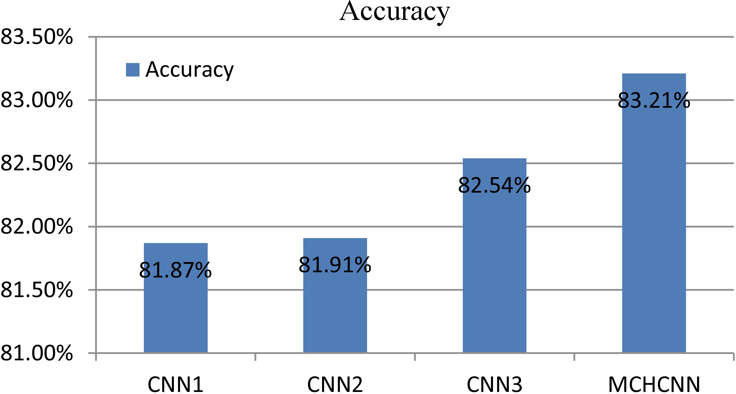

Figure 5.

Caltech-256 dataset experiment results.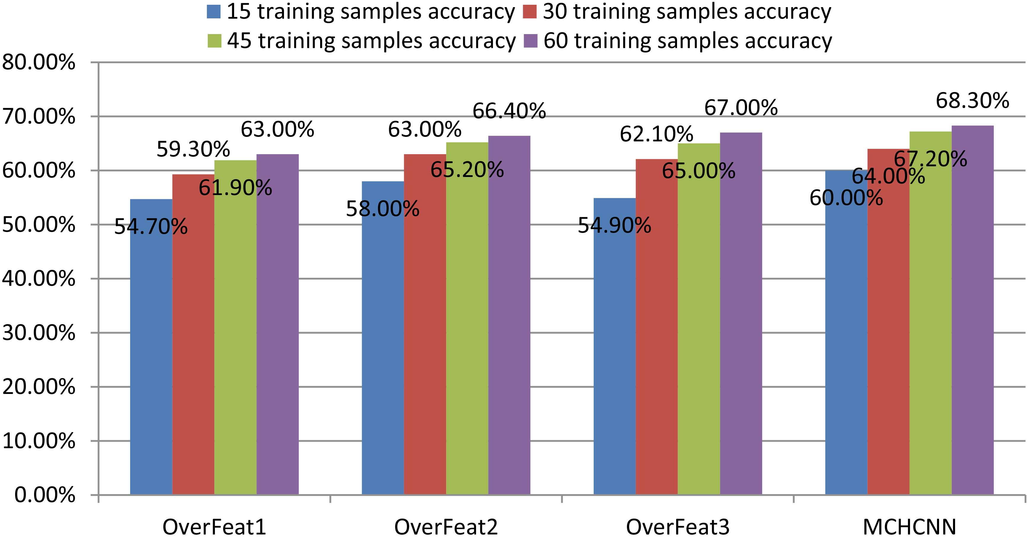

As shown in Fig. 4, the single-column convolutional neural network CNN1, CNN2, and CNN3 achieved 81.87%, 81.91%, and 82.54% accuracy on the CIFAR-10 dataset. The accuracy of MCHCNN is 83.21%, and the accuracy rate is 1.64%, 1.59%, and 0.81% higher than single-column CNN. Experiments based on CIFAR-10 datasets have proved that MCHCNN can achieve better object recognition than single-column CNN.

4.3 Result for Caltech-256

All pictures are scaled to a uniform 221*221 scale by bilinear interpolation to meet OverFeat’s network structure. The experiments are divided into four groups. The number of training samples for each class in each group is 15, 30, 45, and 60. After removing the training set, the remaining pictures of each class are used as test set. In the setting of hyper-parameters, the Grid Search method was used in the experiment to try some parameter combinations, and finally chose the best set of parameters: learning rate $=$ 10 ${}^{-5}$ , momentum $=$ 0.5, weight decay $=$ 10 ${}^{-4}$ . The experimental results are shown in Fig. 5.

As shown in Fig. 5, in these four groups of experiments, MCHCNN has higher accuracy in object recognition on the Caltech-256 dataset than single-column convolutional neural networks. The experimental results are consistent with the previous test in MNIST and CIFAR-10.

Through experiments on MNIST, CIFAR-10 and Caltech-256 datasets, we can conclude that Multi-Column Heterogeneous Convolutional Neural Networks can achieve better object recognition than single-column convolutional neural networks.

5. Conclusion

This paper presents a Multi-Column Heterogeneous Convolutional Neural Network model. The advantage of MCHCNN compared to single-column network is that networks with different structures can learn image features from different perspectives. By changing the network structure of different convolutional neural networks, the differences between the networks are increased, and the diversity of underlying features learning is achieved. Compared with a single convolutional neural network, the object recognition accuracy of the network model can be effectively improved.

Although MCHCNN has a certain improvement in accuracy over a single CNN, it still has some limitations. The design of Multiple-Column Heterogeneous Convolutional Neural Network models is based on some commonly used experience method. There are still some issues that lack of quantitative research. Unable to select the best network structure with accurate quantitative experiments. During the experiment, we also found a problem that in the process of sliding window fusion, the result of four-column network fusion is better than that of six-column network fusion. In other words, sliding window fusion is not a fusion of the network as much as possible. However, we can’t quantify the best number of fused networks.

Quantitative research on Multi-Column Heterogeneous Convolutional Neural Networks is the main research direction in the future. For example, research on the impact of a single convolutional neural network structure (the size of the convolution kernel, the number of feature maps, and the number of layers) on overall network performance; research on how many single convolutional neural networks contained in the network structure will have the best performance; research on the optimal parameters and fusion methods of sliding windows; research on the operating efficiency of the system, etc.

References

Szegedy

Liu

Jia

et al., Going deeper with convolutions, Proceedings of the IEEE Conference on Computer Vision and Pattern Recognition, IEEE Computer Conference on Boston, USA (2015), 1–9.

Lowe

D.G.

, Distinctive Image Features from Scale-Invariant Keypoints, International Journal of Computer Vision 60(2) (2004), 91–110.

Ciresan

Meier

and Schmidhuber

, Multi-column deep neural networks for image classification, Proceedings of IEEE Conference on Computer Vision and Pattern Recognition, Providence (2012), 3642–3649.

Rosten

and Drummond

, Machine Learning for High-speed Corner Detection, Computer Vision-ECCV 2006, Springer Berlin Heidelberg, 2006, 430–443.

Liu

H.M

and Zheng

Z.Q

, Color classification method based on linear classifier for hybrid spatial lookup table, Chinese Journal of Image Graphics 13(1) (2008), 104–108.

Tang

F.X.

and Yang

Y.F.

, Research of color image segmentation algorithm based on asymmetric kernel density estimation, Journal of Computational Methods in Sciences and Engineering 17(3) (2017), 455–462.

Bay

Tuytelaars

and Gool

L.V

, SURF: Speeded Up Robust Features, European Conference on Computer Vision, Springer-Verlag, 2006, 404–417.

Simon

, Neural Network: A Comprehensive Foundation, Neural Networks: A Comprehensive Foundation, Prentice Hall PTR, 1994, 71–80.

K.M

Zhang

X.Y

Ren

S.Q

et al., Deep Residual Learning for Image Recognition, IEEE Conference on Computer Vision and Pattern Recognition, IEEE Computer Society, 2016, 770–778.

10.

Simonyan

and Zisserman

, Very deep convolutional networks for large-scale image recognition, Computer Science, 2014.

11.

Luan

L.H.

and Ji

G.L.

, Research on Decision Tree Classification Technology, Computer Engineering 30(9) (2004), 94–96.

12.

Sonka

Hlavac

and Boyle

, Image processing, analysis, and machine Vision, Beijing: Posts & Tecom Press, 2003.

13.

Haralick

R.M

, Texture features for image classification, IEEE Transactions on Systems Man & Cybemetics, smc-3(6) (1973), 610–621.

14.

Joachims

, Making Large-Scale SVM Learning Parctical, Technische Universitat Dortmund, Sonderforschungsbereich Komplexitatsreduktion in multivariaten Datenstrukturen, 1998, 499–526.

15.

Xue

X.R.

Wang

J.P.

Xiang

and Wang

H.F.

, An efficient method of SAR image segmentation based on texture feature, Journal of Computational Methods in Sciences and Engineering 16(4) (2016), 855–864.

16.

Meng

X.Z.

, Concept-based shape classification and recognition, Computer Engineering and Applications 43(3) (2007), 166–167.

17.

Lecun

Bottou

Bengio

et al., Gradient-based learning applied to document recognition, Proceedings of the IEEE 86(11) (1998), 2278–2324.