Rigid-flexible coupled multi-body dynamics analysis of horizontal directional drilling rig system

Abstract

To reduce the failure probability of gas drainage drilling holes in coal mines, a new modeling method of gas drainage drilling machine is presented. Firstly, each drill pipe is regarded as a flexible body, and the Lagrange’s equation of second kind is used to model it. Secondly, the joint of drill bit, hole wall and drill pipe are regarded as rigid bodies, and the Newton-Euler method is used to model it. Thirdly, the rigid-flexible coupling multi-body dynamic model of drilling rig-drill pipe-hole wall system in medium and short horizontal section of soft coal seam is established by using relative node coordinate method, and the time complexity and operation complexity of modeling are reduced by using ADAMS macro program. Finally, the finite element method is used to discretize the model, and the virtual prototyping technology is used to solve the mathematical model. The simulation results show that the coupling of friction and vibration does not necessarily increase the probability of drilling failure, but sometimes reduces the amplitude of vibration. Compared with the length of each drill pipe, the influence of drilling depth on the system is greater, and the bit-bounce behaviours is more likely to occur in the deep hole. The operating frequency range of the drilling rig is 6.9E-3 to 2.1E+4Hz. When the length of the drill pipe is constant, the natural frequency of the system increases with the increase of the order, while the natural frequency of the deep hole section is almost unaffected by the order. In practical engineering, the vibration excitation of the actuator should be controlled to avoid the natural frequency. Meanwhile, the modal frequency should be avoided as far as possible to reduce the vibration and the failure probability of drilling holes. The model can simulate a series of dynamic responses of drilling rig system in drilling process, and provide theoretical support for subsequent multi-factor coupling modeling.

Keywords

Multi-body dynamics rigid-flexible coupling performance analysis drilling machine friction and vibration

1. Introduction

With the development of mining technology, the increase of drilling rig types and the expansion of mining areas, mining difficulty is also increasing, how to efficiently and safely mine has gradually become the focus of many scholars. Statistics show that in the past 10 years, 389 coal mine gas accidents have occurred in China, with 3307 deaths. Although the frequency of gas accidents is lower than that of transportation accidents, the mortality rate is more than two times. Effective gas extraction can reduce the gas content and pressure to a safe level and eliminate gas disasters fundamentally.

Over the last few years, extensive work has been done to study the borehole failure. In 1979, Bradley proposed a borehole failure model that considers the effect of the wellbore direction on the wellbore and uses the choice of mud weight to prevent wellbore instability [1]. In 1999, Gupta and Zaman proposed an analytical formula for studying the stability of boreholes, the formula is mainly to study the stability of boreholes by analyzing the stress of surrounding rock. It is noteworthy that the anisotropy of materials is considered in this paper [2]. Later, Yuan et al. analyzed the influence of ground stress on the stability of the borehole through a deeper analysis [3, 4, 5, 6]. In general, rock failure criteria are primarily dependent on stress, but there are no fixed criteria for borehole stability analysis, drilling failures are often the result of a combination of factors. Among them, including temperature, friction, vibration, rock strength, topsoil thickness and other factors [7, 8, 9, 10, 11, 12, 13, 14, 15]. With the deepening of research, in recent years, scholars have begun to pay attention to the influence of the coupling of two factors on the drilling system. Among them, Nogueira and Ritto considered the effects of torsional excitation and mud on the system, which modeled by classical torsion theory of finite element method, and stochastic stability diagram is obtained by Monte Carlo method [16]. Divenyi et al. proposed a two-degree-of-freedom lumped parameter model that considers the coupling of axial and torsional vibrations and smoothes the governing equations [17]. Melakhessou et al. established a nonlinear dynamic model of the longitudinal, transverse, and torsional coupling of the drill string system [18]. In addition, scholars have also conducted in-depth research on dynamic modeling and solving methods. Among them, García-Vallejo et al. used finite element method and finite segment method to model the drilling system, and compared the two methods [19]. Arbatani et al. established a rigid-flexible coupling model in which the absolute coordinate method is used to describe the motion of a flexible body, and the natural coordinates are used to describe the rigid body motion [20]. Liang et al. improved the finite element formula by using the node formula and the GT method to integrate the finite element method and the FMD symbol to capture the dynamic hardening effect [21, 22, 23]. Kim et al. improved the multi-body dynamics formula [24, 25, 26, 27].

Due to the diversity and complexity of the rig system and the modeling solution method, it is difficult to fully consider the factors causing the drilling failure. In this paper, the coupling of flexible rods to rigid joints, rigid drill bits and rigid hole walls is considered. At the same time, the influence of friction and vibration on the system is introduced. The rigid-flexible coupling model of the drilling rig system is established by using multi-body dynamics theory, the Friction-Vibration coupling model is established by using the method of Reference [28], in which vibration includes vibration source excitation, friction induced vibration, and eccentricity induced vibration. Compared with the traditional finite element method, the multi-body dynamic method is more efficient and more conducive to the optimization calculation. It is very important to use different methods to calculate the rigid body and flexible body, and consider two kinds of coupling (coupling between rigid body and flexible body and coupling between friction and vibration), which will make the analysis results more accurate. The model can simulate a series of dynamic responses of drilling rig system in drilling process, and provide theoretical support for subsequent multi-factor coupling modeling.

2. Mathematical model

The drilling rig system mainly includes four parts: drilling rig, n-section drill pipe, drilling tool and hole wall. In this paper, the influence of drilling rig and drilling tool structure on the system is not considered, and both of them are assumed to be homogeneous mass blocks. Consider the influence of friction, vibration and the amount of rock intrusion by drill pipe and drill tool on the system. It is assumed that the material of coal, drill pipe and bit are isotropic, at the same time, the error of the parameters such as friction coefficient, elastic modulus and Poisson’s ratio is ignored. The joint of drill bit, coal rock and drill pipe are rigid body, and the drill pipes are flexible body.

2.1 Rigid-flexible coupled model with constraints

Select a set of object coordinate systems $X^{i}_{1},X^{i}_{2},X^{i}_{3}$ , the reference coordinate ${\bm{q}}^{i}_{r}$ is used to represent its position in the global coordinate system $X_{1},X_{2},X_{3}$ .

$\displaystyle\bm{q}^{i}_{r}=[\bm{R}^{i\text{T}}\ \ \bm{\theta}^{i\text{T}}]^{T}$ (1)

where ${\bm{R}}^{i}$ is a set of Cartesian coordinates that determine the origin of an object reference coordinate system. ${\bm{\theta}}^{i}$ is a set of rotational coordinates that describing the position of the object reference coordinate system in the global coordinate system.

Figure 1.

Position of point P on rigid bit.

Figure 2.

Position of $P^{ij}$ on the Flexible Drill pipe.

The position of any point P on the rigid bit in the global coordinate system (Fig. 1) can be written as:

$\displaystyle{\bm{r}}^{i}_{p}={\bm{R}}^{i}+{\bm{A}}^{i}{\overline{\bm{u}}}^{i}$ (2)

where ${\overline{\bm{u}}}^{i}$ is the local position vector of point p. ${\bm{A}}^{i}$ is the transformation matrix from the object coordinate system to the global coordinate system, and values can be expressed by the following equations:

$\displaystyle{\bm{A}}^{i}=\left[\begin{array}[]{cc}\cos{\theta}^{i}&-\sin{% \theta}^{i}\\ \sin{\theta}^{i}&\cos{\theta}^{i}\end{array}\right]$ (3)

The coordinates ${\bm{q}}^{i}$ of flexible drill pipe can be expressed by a set of generalized reference coordinate vectors ${\bm{q}}^{i}_{r}$ and a set of generalized elastic coordinate vectors ${\bm{q}}^{i}_{f}$ as follows:

$\displaystyle{\bm{q}}^{i}=\left[{\bm{R}}^{i\mathrm{T}}\ \ {\bm{\theta}}^{i% \mathrm{T}}\ \ {\bm{q}}^{i\mathrm{T}}_{f}\right]^{T}$ (4)

where ${\bm{R}}^{i}$ , ${\bm{\theta}}^{i}$ are reference coordinates, ${\bm{q}}^{i}_{f}$ is elastic coordinates. The position of any point P on the flexible drill pipe in the whole system can be written as:

$\displaystyle{\bm{r}}^{i}_{p}={\bm{R}}^{i}+{\bm{A}}^{i}{\overline{\bm{u}}}^{i}% ={\bm{R}}^{i}+{\bm{A}}^{i}\left({\overline{\bm{u}}}^{i}_{0}\bm{+}{\bm{S}}^{i}{% \bm{q}}^{i}_{f}\right)$ (5)

Here, ${\overline{\bm{u}}}^{i}_{0}$ is the initial position of point P, ${\bm{S}}^{i}$ is a shape function matrix related to space, ${\bm{S}}^{i}={\bm{S}}^{i}\left(x^{i}_{1},x^{i}_{2},x^{i}_{3}\right)$ .

In order to calculate more accurately, the flexible body is discretized according to the selected finite element method. In order to describe the shape and position of any element in the $j$ th element on the $i$ th drill pipe after discretization conveniently, four Cartesian coordinate systems, namely, the global coordinate system $X Y Z$ , the object coordinate system $X^{i},Y^{i},Z^{i}$ , the element coordinate system $X^{ij}Y^{ij}Z^{ij}$ and the intermediate coordinate system ${\overline{X}}^{ij}{\overline{Y}}^{ij}{\overline{Z}}^{ij}$ , are established respectively. The whole system has nothing to do with time, and unifies the expression of all objects in the system; the object system is fixed on a unit of the $i$ th drill pipe, and unifies the expression of all elements in the object; the element system is fixed on a point of the $j$ unit, and moves with the unit; the intermediate system is fixed on the object system and its initial position is parallel to the element system.

The position of any point $P^{ij}$ on the $j$ th element of the $i$ th flexible drill pipe in the whole system (Fig. 2) can be written as follows:

$\displaystyle{\bm{r}}^{ij}_{p}={\bm{R}}^{i}+{\bm{A}}^{i}{\bm{d}}^{ij}={\bm{R}}% ^{i}+{\bm{A}}^{i}\left({\bm{u}}^{ij}_{0}+{\bm{u}}^{ij}_{f}\right)={\bm{R}}^{i}% +{\bm{A}}^{i}\left({\bm{u}}^{ij}_{0}+{\bm{S}}^{ij}{\bm{q}}^{ij}_{f}\right)$ (6)

where

$\displaystyle{\bm{u}}^{ij}_{f}={\bm{N}}^{ij}{\bm{q}}^{ij}_{f}$ $\displaystyle{\bm{d}}^{ij}={\bm{u}}^{ij}_{0}+{\bm{u}}^{ij}_{f}$ $\displaystyle\ {\bm{S}}^{ij}={\bm{C}}^{ij}{\bm{N}}^{ij}{\overline{\bm{C}}}^{ij}$

${\bm{r}}^{ij}_{p}$ is the position vector of point $P^{ij}$ in the whole system, ${\bm{u}}^{ij}_{f}$ is the elastic deformation vector of point ${P}^{ij}$ in the element coordinate system, ${\bm{q}}^{ij}_{f}$ is the node displacement vector of the element, ${\bm{d}}^{ij}$ is the position of $P^{ij}$ in the system of objects, ${\bm{u}}^{ij}_{0}$ is the position of $P^{ij}$ when it is not deformed in the body system. ${\bm{C}}^{ij}$ is the transformation matrix from the unit coordinate system to the object coordinate system, ${\bm{N}}^{ij}$ is the shape function matrix of the $i j$ th element, ${\overline{\bm{C}}}^{ij}$ is a transformation matrix from object coordinate system to intermediate coordinate system. In the case of small deformation, the transformation matrices ${\bm{C}}^{ij}$ and ${\overline{\bm{C}}}^{ij}$ can be approximated as constant matrices, so the element function matrix ${\bm{N}}^{ij}$ is modified to ${\bm{S}}^{ij}$ , ${\bm{S}}^{ij}$ is a modified matrix of unit functions. The velocity vector of point $P^{ij}$ can be obtained by deriving the time from Eq. (6):

$\displaystyle{\dot{\bm{r}}}^{ij}_{p}={\dot{\bm{R}}}^{i}+{\dot{\bm{A}}}^{i}{\bm% {d}}^{ij}+\bm{A}{\dot{\bm{d}}}^{ij}={\dot{\bm{R}}}^{i}+{\dot{\bm{A}}}^{i}{\bm{% u}}^{ij}_{0}+{\dot{\bm{A}}}^{i}{\bm{u}}^{ij}_{f}+{\bm{A}}^{i}{\bm{S}}^{ij}{% \dot{\bm{q}}}^{ij}_{f}$ (7)

${\bm{A}}^{i}$ can be determined by the angular coordinate ${\bm{\theta}}^{i}$ . Therefore, in the case of $n_{r}$ rotational coordinates, ${\dot{\bm{A}}}^{i}{\bm{d}}^{ij}$ in Eq. (7) can be written as follows:

$\displaystyle{\dot{\bm{A}}}^{i}{\bm{d}}^{ij}={\bm{B}}^{ij}{\dot{\bm{\theta}}}^% {i}$ (8)

where

$\displaystyle{\bm{B}}^{ij}=\left[\frac{\partial}{\partial{\bm{\theta}}^{i}_{1}% }\left({\bm{A}}^{i}{\bm{d}}^{ij}\right)\ \cdots\ \frac{\partial}{\partial{\bm{% \theta}}^{i}_{n_{r}}}\left({\bm{A}}^{i}{\bm{d}}^{ij}\right)\right]$ (9)

Here, ${\dot{\bm{\theta}}}^{i}$ is the derivative of the angular coordinates of an object system with respect to time. The position of $P^{ij}$ in the whole system can be rewritten in block form as follows:

$\displaystyle{\dot{\bm{r}}}^{ij}_{p}=\left[\bm{\mathrm{I}}\ {\bm{B}}^{ij}\ {% \bm{A}}^{i}{\bm{S}}^{ij}\right]\left[\begin{array}[]{c}{\dot{\bm{R}}}^{iT}\\ {\dot{\bm{\theta}}}^{iT}\\ {\dot{\bm{\ }\bm{q}}}^{ijT}_{f}\end{array}\right]={\bm{L}}^{ij}{\dot{\bm{q}}}^% {ij}$ (10)

where $\bm{I}$ is the unit matrix of 3*3. The partitioned form of kinetic energy of the $i$ th flexible drill pipe can be defined as:

$\displaystyle{\bm{E}}^{i}_{p}={\frac{1}{2}\dot{\bm{q}}}^{iT}{\bm{M}}^{i}{\dot{% \bm{q}}}^{i}=\frac{1}{2}{\left[\begin{array}[]{c}{\dot{\bm{R}}}^{i}\\ {\dot{\bm{\theta}}}^{i}\\ {\dot{\bm{q}}}^{i}_{f}\end{array}\right]}^{T}\left[\begin{array}[]{ccc}m^{ij}_% {RR}&m^{ij}_{R\theta}&m^{ij}_{Rf}\\ m^{ijT}_{\theta f}&m^{ij}_{\theta\theta}&m^{ij}_{\theta f}\\ m^{ijT}_{Rf}&m^{ijT}_{R\theta}&m^{ij}_{ff}\end{array}\right]\left[\begin{array% }[]{c}{\dot{\bm{R}}}^{i}\\ {\dot{\bm{\theta}}}^{i}\\ {\dot{\bm{q}}}^{i}_{f}\end{array}\right]$ (11)

where ${\bm{E}}^{i}_{p}$ is the kinetic energy of drill pipe I in a multibody system, $m^{ij}_{RR}$ is the inertial tensor of the element translating relative to the object system, $m^{ij}_{R\theta}$ is the inertial coupling between translation and rotation of the body system, $m^{ij}_{Rf}$ is the coupling of the translation of the body system and the elastic deformation of the element, $m^{ij}_{\theta\theta}$ is the inertial tensor of the element rotating relative to the body system, $m^{ij}_{\theta f}$ is the inertial coupling between the rotation of the body system and the elastic deformation of the element, $m^{ij}_{ff}$ is the inertial tensor of the elastic deformation of the element relative to the body system. Using the element stiffness set method in finite element method and considering the block form of reference coordinates and elastic coordinates, the block form of strain energy of the $i$ th flexible drill pipe can be defined as:

$\displaystyle{\bm{U}}^{\bm{i}}=-\frac{1}{2}{\bm{q}}^{iT}_{f}{\bm{K}}^{i}_{ff}{% \bm{q}}^{i}_{f}=-\frac{1}{2}{\left[\begin{array}[]{c}{\bm{R}}^{iT}\\ {\bm{\theta}}^{iT}\\ {\bm{q}}^{iT}_{f}\end{array}\right]}^{T}\left[\begin{array}[]{ccc}0&0&0\\ 0&0&0\\ 0&0&{\bm{K}}^{i}_{ff}\end{array}\right]\left[\begin{array}[]{c}{\bm{R}}^{iT}\\ {\bm{\theta}}^{iT}\\ {\bm{q}}^{iT}_{f}\end{array}\right]$ (12)

where ${\bm{K}}^{i}_{ff}$ is a symmetric positive definite stiffness matrix related to the elastic coordinates of element $i j$ , ${\bm{K}}^{i}_{ff}=\textit{diag}\left({\bm{K}}^{i1}_{ff},{\bm{K}}^{i2}_{ff},% \ldots,{\bm{K}}^{in_{e}}_{ff}\right)$ . The virtual work of all external forces acting on the $i$ th flexible drill pipe can be expressed as:

$\displaystyle\delta{\bm{W}}^{i}_{e}={\bm{Q}}^{iT}_{e}\delta{\bm{q}}^{i}$ (13)

where ${\bm{Q}}^{i}_{e}$ is all the generalized force vectors related to the generalized coordinates except the reactive power constraints between the drill pipes, Subscript e is external force. The virtual work of all the forces on the $i$ th drill pipe can be obtained by adding the virtual work (strain energy) of the elastic force caused by the deformation of drill pipe and the virtual work of all the external forces acting on the drill pipe:

$\displaystyle\delta{\bm{W}}^{i}=\delta{\bm{U}}^{\bm{i}}\bm{+}\delta{\bm{W}}^{i% }_{e}$ (14)

where $\delta{\bm{W}}^{i}$ is the virtual work of all forces acting on the $i$ th drill pipe, $\delta{\bm{U}}^{\bm{i}}$ is the virtual work of elastic force caused by deformation, $\delta{\bm{W}}^{i}_{e}$ is the virtual work of external force. According to Eqs (12)–(14) can be written as follows:

$\displaystyle\delta{\bm{W}}^{i}=-{\bm{q}}^{iT}{\bm{K}}^{i}\delta{\bm{q}}^{i}+{% \bm{Q}}^{iT}_{e}\delta{\bm{q}}^{i}={\bm{Q}}^{iT}\delta{\bm{q}}^{i}$ (15) $\displaystyle\bm{Q}^{i}=-{\bm{q}}^{i}{\bm{k}}^{i}+\bm{Q}^{i}_{e}$ (16)

where ${\bm{Q}}^{i}$ is a generalized force vector related to the generalized coordinates of drill pipe $i$ . From the kinetic energy and generalized force vector of drill pipe $i$ , the Lagrange equation can be derived as follows:

$\displaystyle\frac{d}{dt}{\left(\frac{\partial{\bm{E}}^{i}_{p}}{\partial{\bm{q% }}^{i}}\right)}^{T}-{\left(\frac{\partial{\bm{E}}^{i}_{p}}{\partial{\bm{q}}^{i% }}\right)}^{T}={\bm{Q}}^{i}$ (17)

where ${\bm{E}}^{i}_{p}$ is the kinetic energy of drill pipe $i$ . The dynamic equation of flexible drill pipe $i$ can be further written as follows:

$\displaystyle{\bm{M}}^{i}{\ddot{\bm{q}}}^{i}\bm{+}{\bm{K}}^{i}{\bm{q}}^{i}={% \bm{Q}}^{i}_{e}+{\bm{Q}}^{i}_{v}$ (18)

where ${\bm{Q}}^{i}_{v}$ is a velocity quadratic vector related to the generalized coordinates of drill pipe $i$ .

The constraint equation derived from holonomic constraints is:

$\displaystyle\bm{C}\left(\bm{q},t\right)=\bm{C}\left(q_{1},q_{2},\ldots,q_{n},% t\right)=0$ (19)

Constraint equations derived from nonholonomic constraints are usually written as

$\displaystyle\bm{C}\left(\bm{q},\dot{\bm{q}},t\right)=0$ (20)

where

$\displaystyle\bm{C}={\left[C_{1}\left(q,t\right)\ C_{2}\left(q,t\right)\ % \ldots\ C_{n_{c}}\left(q,t\right)\right]}^{T}$ (21) $\displaystyle\bm{q}={\left[q_{1}\ q_{2}\ \ldots\ q_{n}\right]}^{T}=0$ (22)

where $\bm{C}$ is an independent system of constrained equations, $\bm{q}$ is the generalized coordinate vector of the system. Considering the holonomic constraints and nonholonomic constraints, the differential equations of motion of the drill pipe are obtained according to the Darumber principle:

$\displaystyle\frac{d}{dt}{\left(\frac{\partial{\bm{E}}^{i}_{p}}{\partial\dot{% \bm{q}}}\right)}^{T}-{\left(\frac{\partial{\bm{E}}^{i}_{p}}{\partial\bm{q}}% \right)}^{T}+{\bm{C}}^{T}_{q}\bm{\lambda}=\bm{Q}$ (23)

in which $\bm{\lambda}={\left[{\lambda}_{1}\ {\lambda}_{2}\ \ldots\ {\lambda}_{nc}\right% ]}^{T}$ is a Lagrange multiplier vector, ${\bm{C}}_{q}$ is a constrained Jacobian matrix, which is an $n_{c}\times n$ -order matrix, ${\bm{E}}^{i}_{p}$ is the kinetic energy of the system, $\bm{Q}$ is the generalized force vector of the system. Considering the contact between drill pipe and coal and coal rock, the total virtual work on drill pipe $i$ is:

$\displaystyle\delta{\bm{W}}^{i}=\delta{\bm{W}}^{i}_{s}+\delta{\bm{W}}^{i}_{e}+% \delta{\bm{W}}^{i}_{c}$ (24)

where $\delta{\bm{W}}^{i}_{s}$ is the virtual work of internal force caused by elastic deformation, $\delta{\bm{W}}^{i}_{e}$ is the virtual work of external force, $\delta{\bm{W}}^{i}_{c}$ is the virtual work of contact force.

$\displaystyle\delta{\bm{W}}_{c}=\left(\sum^{\textit{Lcstick}}_{\textit{stick}=% 1}{{\bm{Q}}_{\textit{cstick}}+}\sum^{\textit{Lcslid}}_{\textit{slid}=1}{{\bm{Q% }}_{\textit{cslid}}}\right)\delta\bm{q}={\bm{Q}}_{c}\delta\bm{q}$ (25) $\displaystyle{\bm{Q}}_{c}=\sum^{\textit{Lcstick}}_{\textit{stick}=1}{{\bm{Q}}_% {\textit{cstick}}+}\sum^{\textit{Lcslid}}_{\textit{slid}=1}{{\bm{Q}}_{\textit{% cslid}}}$ (26)

where ${\bm{Q}}_{\textit{cstick}}$ is a generalized constraint for viscous contact, ${\bm{Q}}_{\textit{cslid}}$ is a generalized constraint for sliding contact, ${\bm{Q}}_{c}$ is a generalized contact force. From the fact that the force between contact points is equal in magnitude and opposite in direction, the dynamic model can be obtained as follows. It is a rigid flexible coupling dynamic model of drilling rig system, which includes ideal constraint, viscous contact and sliding contact.

$\displaystyle\bm{M}\ddot{\bm{q}}+\bm{Kq}-{\bm{Q}}_{e}-{\bm{Q}}_{v}+{\bm{C}}^{T% }_{q\left(\textit{tst}\right)}{\lambda}_{\textit{tst}}+{\bm{C}}^{T}_{q\left(% \textit{tsl}\right)}{\lambda}^{T}_{\textit{tsl}}{\bm{C}}_{q\left(\textit{tsl}% \right)}+{\bm{C}}^{T}_{q\left(\textit{ide}\right)}{\lambda}_{\textit{ide}}=0$ (27)

where ${\bm{Q}}_{e}$ is the generalized external force of the system, ${\bm{Q}}_{v}$ is the velocity quadratic vector of the system, ${\bm{C}}_{q}\left(\textit{tst}\right)$ , ${\bm{C}}_{q}\left(\textit{tsl}\right)$ and ${\bm{C}}_{q}\left(\textit{ide}\right)$ respectively represent the Jacobian matrix of the viscous, sliding, and ideal constraint equations, $λ_{\textit{tst}}$ , $λ_{\textit{tsl}}$ and $λ_{\textit{ide}}$ respectively represent the binding reaction forces of sticky, sliding, and ideal constraints.

$\displaystyle\lambda={\left({\lambda}_{\textit{tst}}\ {\lambda}_{\textit{tsl}}% \ {\lambda}_{\textit{ide}}\right)}^{T}$ (28) $\displaystyle{\widetilde{\bm{C}}}^{T}_{q}=\left({\bm{C}}^{T}_{q\left(\textit{% tst}\right)}\ {\bm{C}}^{T}_{q\left(\textit{tsl}\right)}\ {\bm{C}}^{T}_{q(% \textit{ide})}\right)$ (29)

Considering Eqs (28) and (29), Eq. (27) can be rewritten as:

$\displaystyle\bm{M}\ddot{\bm{q}}+\bm{Kq}-{\bm{Q}}_{e}-{\bm{Q}}_{v}+{\widetilde% {\bm{C}}}^{T}_{q}\lambda=0$ (30)

The constraint equation is:

$\displaystyle\widetilde{\bm{C}}\left(\bm{R},\bm{\theta},{\bm{q}}_{f},\bm{t}% \right)=0$ (31)

2.2 Friction and vibration model

The sliding friction ${\bm{F}}_{f}$ acting on the contact point can be given by Coulomb friction. The expressions are as follows:

$\displaystyle{\bm{F}}_{f}=\left\{\begin{array}[]{lc}-\mu{\bm{F}}_{N},&\dot{\bm% {q}}_{h}>0\\ -{\mu}_{s}{\bm{F}}_{N},&\dot{\bm{q}}_{h}=0\\ {\bm{F}}_{N},&\dot{\bm{q}}_{h}<0\end{array}\right.$ (32)

where

$\displaystyle{\bm{F}}_{N}=\bm{K}{\delta}^{e}+C_{1}\dot{\delta}+C_{2}\dot{% \delta}\delta$ (33)

where ${\bm{F}}_{f}$ is friction, ${\bm{F}}_{N}$ is the normal force between contact points, $\mu$ is the dynamic friction coefficient between contact points, ${\mu}_{s}$ is the maximum static friction coefficient, ${\bm{q}}_{h}$ is the relative sliding velocity between contact points, $\bm{K}$ is contact stiffness, $C_{1}$ and $C_{2}$ are damping factors, $\delta$ is the normal penetration distance of the contact point. When there is no relative slip between the system and the rock strata, $F_{f}$ is between $-{\mu}_{s}{\bm{F}}_{N}$ and ${\mu}_{s}{\bm{F}}_{N}$ . For the convenience of calculation, the friction formula can be rewritten as follows:

$\displaystyle{\bm{F}}_{f}=-\mu{\bm{F}}_{N}\text{Sign}(\dot{\bm{q}}_{h})$ (34)

where $\text{Sign}\left(\cdot\right)$ is a symbolic function

$\displaystyle\text{Sign}\left(\cdot\right)=\left\{\begin{array}[]{ll}+1,&{\bm{% q}}_{h}>0\\ \left[+1,\ -1\right],&{\bm{q}}_{h}=0\\ -1,&{\bm{q}}_{h}<0\end{array}\right.$

In order to avoid the rigidity caused by discontinuity in friction calculation, a smoothing function is introduced to modify the dynamic friction force.

$\displaystyle{\bm{F}}_{f}=-\text{Sign}({\dot{\bm{q}}}_{h})\left(\frac{2}{\pi}% \right)\text{arctan}\left(\varepsilon{\dot{\bm{q}}}_{h}\right)\left(\frac{\mu-% {\mu}_{s}}{1+\tau\left|{\dot{\bm{q}}}_{h}\right|}+\mu\right)$ (35)

where $\varepsilon$ and $\tau$ are smoothing coefficients and dimensionless numerical constants. Rolling friction can be written as:

$\displaystyle{\bm{F}}_{r}={\delta}_{r}{\bm{F}}_{N}$ (36)

where ${\delta}_{r}$ is the rolling friction coefficient.

The centrifugal force acting on the drill pipe can be written as:

$\displaystyle{\bm{F}}_{R}=me\left(\frac{\pi\omega}{30}\right)$ (37)

where $m$ is the quality of a single drill pipe, $e$ is eccentricity, $\omega$ is the rotation rate. Assuming that the deflection at the cross section is positive upward, the differential equation of the transverse vibration of the bar can be written as follows:

$\displaystyle{\bm{F}}_{H}\left(\bm{q},t\right)={\bm{E}}_{w}{\bm{I}}_{p}\frac{{% \partial}^{4}\bm{y}}{{\partial\bm{q}}^{4}}+C_{s}I\frac{{\partial}^{5}\bm{y}}{{% \partial\bm{q}}^{4}\partial t}+\rho A\frac{{\partial}^{2}\bm{y}}{{\partial\bm{% q}}^{2}}$ (38)

where ${\bm{E}}_{w}{\bm{I}}_{p}$ I is bending stiffness, ${\bm{F}}_{H}\left(\bm{q},t\right)$ is the transverse force applied to the drill pipe, $\bm{y}\left(\bm{q},t\right)$ is the transverse displacement of the cross section at time t, $C_{s}$ is the strain internal damping coefficient, $\rho$ is the density of drill pipe, $A$ is the cross-sectional area. The axial vibration equation of drill pipe can be written as follows:

$\displaystyle{\bm{E}}_{l}{\bm{I}}_{p}\frac{{\partial}^{2}\bm{u}}{{\partial t}^% {2}}=\rho A\frac{{\partial}^{2}\bm{u}}{{\partial\bm{q}}^{2}}$ (39)

where ${\bm{E}}_{l}{\bm{I}}_{p}$ is tension-compression stiffness, $\bm{u}\left(\bm{q},t\right)$ is the axial displacement of cross section at time $t$ . The torsional vibration equation of drill pipe can be written as follows:

$\displaystyle\bm{G}{\bm{I}}_{p}\frac{{\partial}^{2}\bm{\theta}}{{\partial t}^{% 2}}=\rho A\frac{{\partial}^{2}\bm{\theta}}{{\partial\bm{q}}^{2}}$ (40)

where $\bm{G}$ is the shear modulus of materials, ${\bm{I}}_{p}$ is the moment of polar inertia of the drill pipe’s circular section to the center point, $\bm{G}{\bm{I}}_{p}$ is torsional stiffness, $\bm{\theta}\left(\bm{q},t\right)$ is the angular displacement of the section at time $t$ . It can be seen from document 28 that friction and vibration affect each other, so the coupling term after friction and vibration coupling is written as follows:

$\displaystyle{\bm{F}}_{mz}=\sqrt{{{\bm{F}}^{2}_{f}+{\bm{F}}^{2}_{r}+{\bm{F}}^{% 2}_{R}+\left({\bm{E}}_{w}{\bm{I}}_{p}\bm{y}\right)}^{2}+{\left({\bm{E}}_{l}{% \bm{I}}_{p}\bm{u}\right)}^{2}+\left(\bm{G}{\bm{I}}_{p}\bm{\theta}\right)}$ (41)

Equation (30) can be rewritten as:

$\displaystyle\bm{M}\ddot{\bm{q}}\bm{+}\bm{Kq}-{\bm{Q}}_{e}-{\bm{Q}}_{v}-{\bm{F% }}_{mz}+{\widetilde{\bm{C}}}^{T}_{q}\lambda=0$ (42)

2.3 Boundary condition

After contact collision, there are three kinds of conditions for drill pipe unit: velocity reversal, velocity equal to the product of velocity and recovery coefficient before collision, and drill pipe will be separated from the hole wall.

The boundary conditions can be established as follows:

$\displaystyle\left\{\begin{array}[]{l}{\dot{\bm{q}}}^{i-}_{z}=-\lambda{\dot{% \bm{q}}}^{i+}_{z}\\ {\dot{\bm{q}}}^{i-}_{y}=-\lambda{\dot{\bm{q}}}^{i+}_{y}\\ {\bm{q}}^{i-}_{z}=\left(1-\delta\right){\bm{q}}^{i+}_{z}\\ \ {\bm{q}}^{i-}_{y}=\left(1-\delta\right){\bm{q}}^{i+}_{y}\\ {\ddot{\bm{q}}}^{i-}_{z}={\ddot{\bm{q}}}^{i}_{2z}\\ {\ddot{\bm{q}}}^{i-}_{y}={\ddot{\bm{q}}}^{i}_{2y}\\ {\bm{M}}^{i}_{e}=-{\bm{F}}^{i}_{N}\left(\mu+{\delta}_{r}\right)R^{i}_{r}\end{% array}\right.$ $\displaystyle{\ddot{\bm{q}}}^{i}_{2z}=\frac{{\dot{\bm{q}}}^{i2}_{2}}{2\Delta}% \frac{{\bm{q}}^{i2}_{z}}{\sqrt{{\bm{q}}^{i2}_{y}+{\bm{q}}^{i2}_{z}}}$ (43) $\displaystyle{\ddot{\bm{q}}}^{i}_{2y}=\frac{{\dot{\bm{q}}}^{i2}_{2}}{2\Delta}% \frac{{\bm{q}}^{i2}_{y}}{\sqrt{{\bm{q}}^{i2}_{y}+{\bm{q}}^{i2}_{z}}}$

where $+$ stands for pre-collision, – stands for post-collision, subscripts $x$ , $y$ and $z$ denote three directions of $X$ , $Y$ and $Z$ , respectively, $\delta$ is a minimal positive number, ${\ddot{\bm{q}}}^{i}_{2z}$ and ${\ddot{\bm{q}}}^{i}_{2y}$ are accelerations of drill pipe units in the collision and recovery stages respectively, ${\bm{M}}^{i}_{e}$ is the friction moment produced by the contact between drill pipe element and rock stratum, ${\bm{F}}^{i}_{N}$ is the positive pressure of the contact point in contact collision, $\mu$ and ${\delta}_{r}$ are the sliding and rolling friction coefficients of drill pipe and coal rock in contact, respectively, $R^{i}_{r}$ is the drilling radius of the collision, $\Delta$ is the extrusion deformation of coal rock, ${\dot{\bm{q}}}^{i}_{2}$ is the velocity after collision.

3. Numerical simulation

3.1 Static solution

When the system is stationary, the dynamic model can be rewritten as follows:

$\displaystyle\bm{Kq}+{\widetilde{\bm{C}}}^{T}_{q}\lambda={\bm{Q}}_{e}$ (44) $\displaystyle\widetilde{\bm{C}}\left(\bm{q},\bm{t}\right)=0$

$\displaystyle{\bm{R}}_{e}={\bm{Q}}_{e}\bm{-}\bm{Kq}$ (45)

Write the generalized coordinates into chunks of the form:

$\displaystyle\bm{q}=\left[{\bm{q}}^{T}_{i}\ \ {\bm{q}}^{T}_{d}\right]^{T}$ (46)

where ${\bm{q}}_{i}$ and ${\bm{q}}_{d}$ represent generalized independent coordinates and related coordinates, respectively. Find the partial derivative of the constraint equation to the generalized coordinates and write it in a compact form:

$\displaystyle{\widetilde{\bm{C}}}_{q}\cdot\delta\bm{q}=0$ (47)

Write Eq. (47) as an independent coordinate, the relevant coordinate block form is:

$\displaystyle{\widetilde{\bm{C}}}_{qi}\delta{\bm{q}}_{i}\bm{+}{\widetilde{\bm{% C}}}_{qd}\delta{\bm{q}}_{d}=0$ (48)

where ${\bm{C}}_{qd}$ is a matrix of order $n_{c}\times n_{c}$ , ${\bm{C}}_{qi}$ is a matrix of order $n_{c}\times\left({n-n}_{c}\right)$ , $n_{c}$ is an independent number of constrained equations, $n$ is a generalized coordinate number. The virtual displacement of the general generalized coordinates can be expressed as:

$\displaystyle\delta\bm{q}=\left[\begin{array}[]{c}\delta{\bm{q}}_{i}\\ \delta{\bm{q}}_{d}\end{array}\right]=\left[\begin{array}[]{c}\bm{I}\\ {\bm{C}}_{\bm{di}}\end{array}\right]\delta{\bm{q}}_{i}={\bm{E}}_{\bm{di}}% \delta{\bm{q}}_{i}$ (49)

where ${\bm{E}}_{\bm{di}}$ is $n\times\left({n-n}_{c}\right)$ order matrix. Substituting Eq. (45) into Eq. (44), multiplying both sides by a virtual displacement, and considering Eqs (47) and (49):

$\displaystyle-{\bm{R}}^{T}_{e}{\bm{E}}_{\bm{di}}=0$ (50)

${\bm{q}}_{i}$ can be obtained by solving Eq. (50).

When

$\displaystyle\overline{\bm{R}}=-{\bm{R}}^{T}_{e}{\bm{E}}_{\bm{di}}$ (51)

Then

$\displaystyle\frac{\partial\overline{\bm{R}}}{\partial{\bm{q}}_{i}}\Delta{\bm{% q}}_{i}=-\overline{\bm{R}}$ (52)

Solution Eq. (52) can obtain $\Delta{\bm{q}}_{i}$ , where $\frac{\partial\overline{\bm{R}}}{\partial{\bm{q}}_{i}}$ can be calculated by difference method to determine all independent coordinates ${\bm{q}}_{i}$ , at the same time, the Newton-Raphson method can be used to solve the constraint equation to obtain the relevant coordinates ${\bm{q}}_{d}$ . Therefore, the general coordinate vector can be written as follows:

$\displaystyle\bm{q}=\left[{\bm{q}}^{T}_{i}\ \ {\bm{q}}^{T}_{d}\right]^{T}$ (53)

3.2 Kinematics solution

Similar to the generalized coordinates, the generalized velocity can be divided into two parts.

$\displaystyle\dot{\bm{q}}=\left[{\dot{\bm{q}}}^{T}_{i}\ \ {\dot{\bm{q}}}^{T}_{% d}\right]^{T}$ (54)

Find the partial derivative of the constraint equation to time, and write it in block form as follows:

$\displaystyle{\widetilde{\bm{C}}}_{qi}{\dot{\bm{q}}}_{i}\bm{+}{\widetilde{\bm{% C}}}_{qd}{\dot{\bm{q}}}_{d}\bm{+}{\widetilde{\bm{C}}}_{t}=0$ (55)

where ${\widetilde{\bm{C}}}_{t}$ is the first derivative of the constraint equation with respect to time. The independent generalized velocity can be obtained by deriving the time, and the generalized velocity vector can be obtained by solving the Eq. (55).

Figure 3.

Overall flow chart.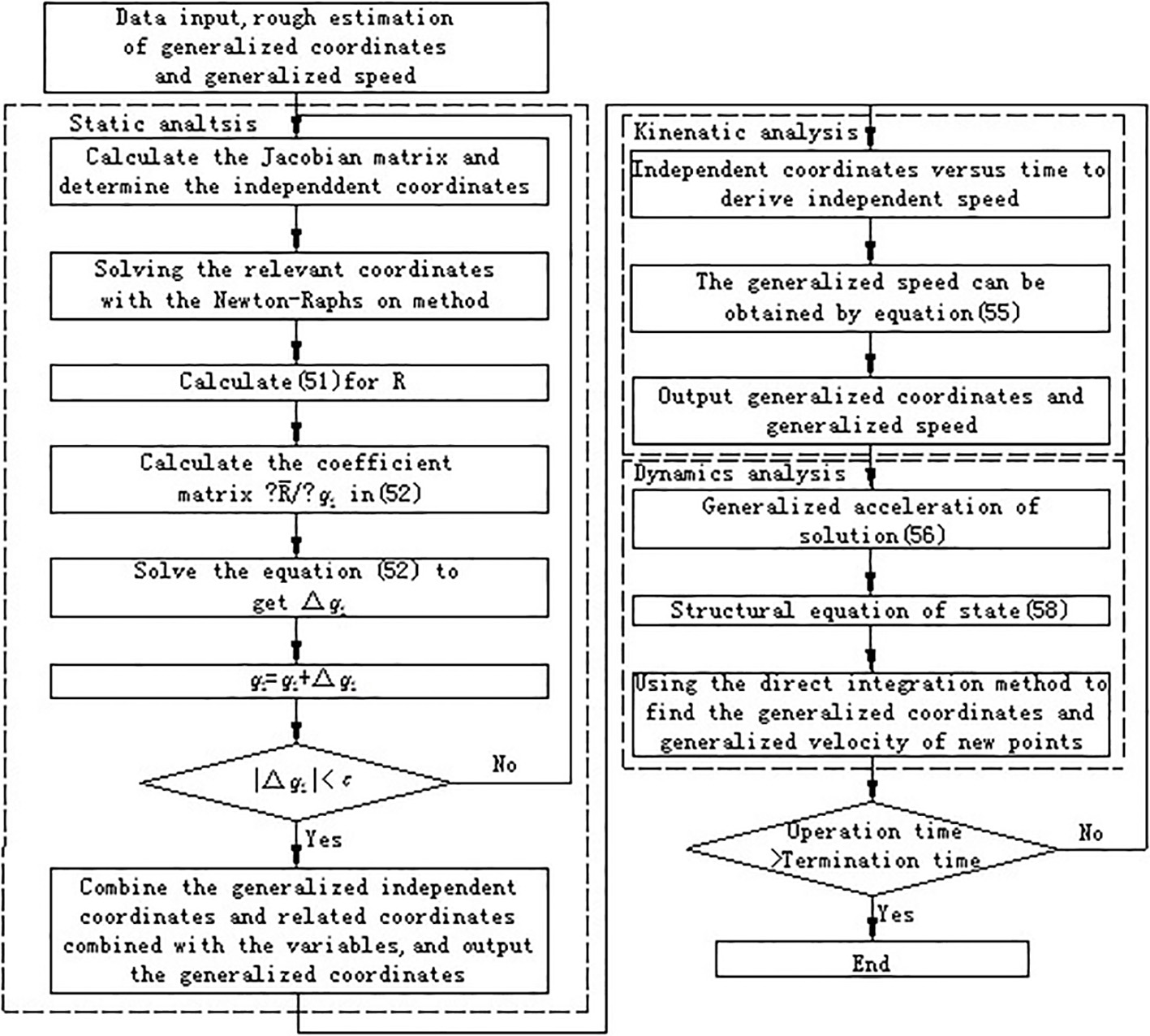

3.3 Dynamics solution

The quadratic partial derivative of the constraint equation for time is obtained and combined with the multi-body dynamic equation.

$\displaystyle\left[\begin{array}[]{cc}\bm{M}&{\widetilde{\bm{C}}}^{T}_{q}\\ {\widetilde{\bm{C}}}_{q}&0\end{array}\right]\left[\begin{array}[]{c}\ddot{\bm{% q}}\\ \lambda\end{array}\right]=\left[\begin{array}[]{c}{\bm{Q}}_{e}+{\bm{Q}}_{v}+{% \bm{F}}_{mz}-\bm{Kq}\\ -{\widetilde{\bm{C}}}_{tt}-2{\widetilde{\bm{C}}}_{qt}\dot{\bm{q}}-{\left({% \widetilde{\bm{C}}}_{q}\dot{\bm{q}}\right)}_{\bm{q}}\dot{\bm{q}}\end{array}\right]$ (56)

where ${\widetilde{\bm{C}}}_{q}$ is the Jacobian matrix of the constrained equation, ${\widetilde{\bm{C}}}_{tt}$ is the quadratic derivative of the constraint equation with respect to time, Therefore, $\ddot{\bm{q}}=f\left(\bm{q},\dot{\bm{q}},t\right)$ can be derived from the above formula. Similar to the generalized coordinates, the generalized acceleration can be divided into two parts.

$\displaystyle\ddot{\bm{q}}=\left[{\ddot{\bm{q}}}^{T}_{i}\ \ {\ddot{\bm{q}}}^{T% }_{d}\right]^{T}$ (57)

The equation of state can be constructed as:

$\displaystyle\bm{H}=\left[{\bm{q}}^{T}_{i}\ \ {\dot{\bm{q}}}^{T}_{i}\right]^{T}$ (58) $\displaystyle\dot{\bm{H}}={\left[{\dot{\bm{q}}}^{T}_{i}\ \ {\ddot{\bm{q}}}^{% \bm{T}}_{\bm{i}}\right]}^{\bm{T}}$

The generalized acceleration is solved by the Eq. (56), and it is returned to the Eq. (3.3), the generalized velocity and the generalized coordinates of the next point are obtained by the direct integration method.

The overall flow chart is as follows (see Fig. 3).

Table 1

System parameters

Each drill rod length	1500 mm	Rod inner diameter	$\Phi$ 63.5 mm
Drill diameter	$\Phi$ 94 mm	Rod outer diameter	$\Phi$ 73 mm
Rate of penetration	10 mm/s	Rotating speed	1501.2 ${}^{\circ}$ /s
Feed pressure	2.96 mpa	Rolling friction coefficient	0.03
Static friction coefficient	0.4	Dynamic friction coefficient	0.36
$\varepsilon$	10 ${}^{4}$	$\tau$	10.9
Drill pipe material parameters:
Elastic modulus		212 GPa
Poisson’s ratio		0.28
Density		7.85 g/cm ${}^{3}$
Bit material parameters:
Elastic modulus		190 GPa
Poisson’s ratio		0.3
Density		7.75 g/cm ${}^{3}$
Soft rock formation parameters:
Elastic modulus		0.05 GPa
Poisson’s ratio		0.28
Density		768 kg/m ${}^{3}$
Shear modulus		65 GPa
Bulk modulus		1.04 GPa
Friction angle		20 ${}^{\circ}$

4. Global dynamics analysis

In this section, numerical results obtained using the proposed model are discussed. The model needs to be validated before solving. The validation module of Adams shows that the model has two rigid components, 100 flexible rods, a pair of motions, 101 fixed constraints, two actuators and 2200 degrees of freedom, without Over-constrained and under-constrained. Because there are too many components and constraints, modeling with macro programming can greatly reduce modeling effort and modeling time.

Figure 4.

Z-axis displacement of rigid system bit.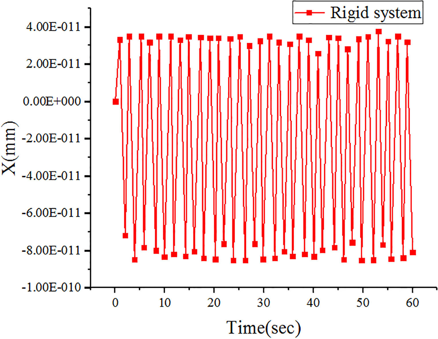

Figure 5.

Z-axis displacement of drill bit in rigid-flexible coupling system.

The difference between the two figures is caused by the different modeling methods. The displacement of the bit along the Z-axis in the rigid system is shown in the Fig. 4. It can be seen that the displacement curve of the bit is not divided by the X-axis, but the amplitude under the X-axis is larger than that above the X-axis, and the fluctuation curve shows some regularity. The displacement of the drill bit in the Z-axis in a rigid-flexible coupling system is shown in the Fig. 5. Since the drill bit is rigid in both systems, the curve difference is caused by the coupling of the drill pipe. The rigid-flexible coupling system is greatly affected by gravity, and it is far from the X-axis, and there is no obvious law. The sudden increase and decrease of the amplitude occurs sometimes, which is more in line with the actual working conditions.

Figure 6.

Kinetic energy of the 100th drill pipe in 3 cases.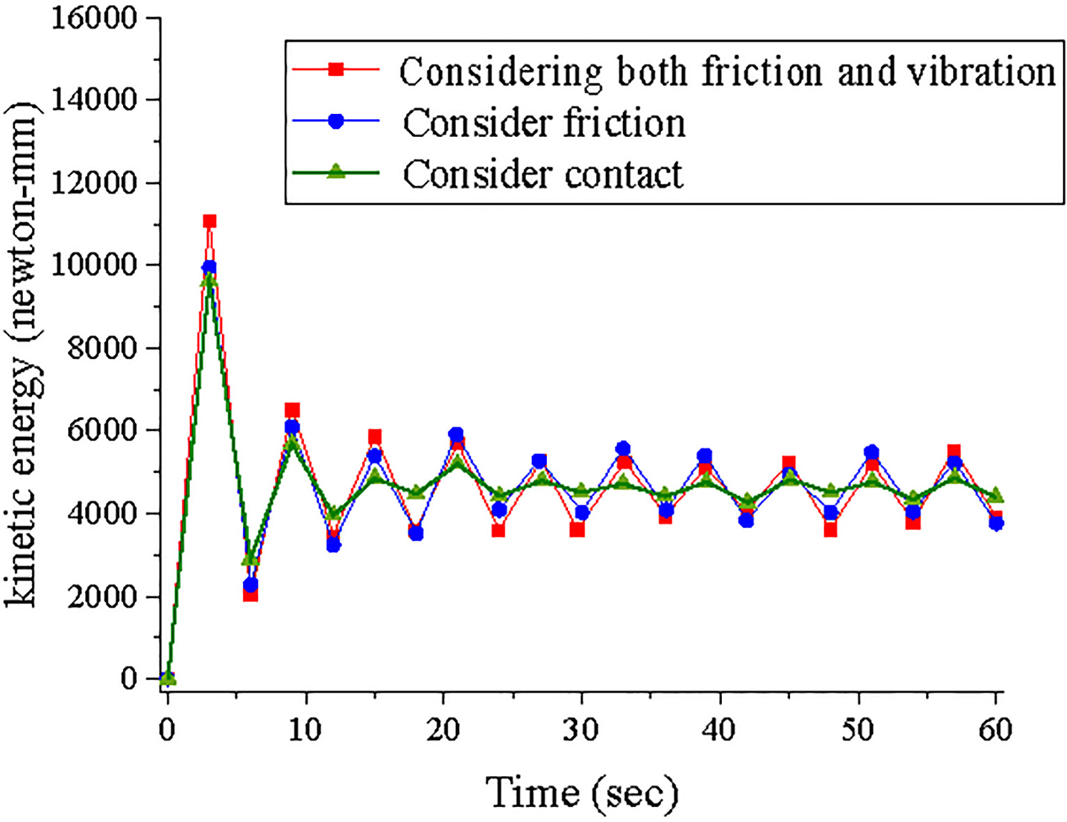

A comparison of the kinetic energy of the 100th flexible rod of the drill pipe is shown in the Fig. 6. The differences among the three curves are caused by different factors. The red line with square symbol (curve 1 ) considers the influence of friction and vibration on the system, blue line with circle symbol (curve 2 ) only considers the influence of friction on the system, and green line with triangle symbol (curve 3 ) only considers the influence of contact on the system.

Throughout the whole picture, curve 3 has the best stability compared with curves 1, 2, friction and vibration will not only increase the kinetic energy amplitude, but also the amplitude sudden increase and sudden drop instability, which may lead to the occurrence of an emergency. In general, curve 1 is slightly larger than the curve 2, and microscopically, in some places, curve 2 fluctuates slightly more than curve 1, which indicates that friction and vibration coupling not only cause the force to be intensified, but also reduce the force.

When the rig is drilling, the kinetic energy of the drill pipe is the largest. The kinetic energy is continuously attenuated within 10 s, and then gradually stabilizes. After 15 s, the data has basically become stable. Therefore, the simulation should not only focus on the analysis of data within 10 s, but also need to extend the simulation time appropriately to more accurately simulate the entire drilling process. In summary, the analysis of the data within 20 s is most appropriate. Therefore, in order to reduce the calculation amount, save the calculation time, enrich the calculation content, and better simulate the whole drilling process, the subsequent simulation only calculates the friction and vibration, and set all analysis time to 20 seconds.

This section mainly analyzes the rigid-flexible coupling model considering friction and vibration. The friction includes contact collision and Coulomb friction. The vibration includes vibration of the driving source, vibration caused by friction and vibration caused by eccentricity. According to the previous analysis, the rigid-flexible coupling model considering friction and vibration is modified, including:

(1)

In order to simulate the rig movement more accurately, the rotary drive and the translation drive are divided into six stages: 0–1 s rig start; 1–19 s drill down; 19–20 s stop rotation and peace at the same time; 20 s–21 s remain static 21–22 s rig reverse start; 22–40 s draw drill.

Translational motion parameter program: STEP (time, 0, 0, 1, – 10) $+$ STEP (time, 1, 0, 19, 0) $+$ STEP (time, 19, 0, 20, 10) $+$ STEP (time, 20, 0, 21, 0) $+$ STEP (time, 21, 0, 22, 10) $+$ STEP (time, 22, 0, 40, 0).

Similarly, the parameters of the rotation motion can be written as: STEP (time, 0, 0 d, 1, $-$ 1501.2 d) $+$ STEP (time, 1, 0 d, 19, 0 d) $+$ STEP (time, 19, 0 d, 20, 1501.2 d) $+$ STEP (time, 20, 0 d, 21, 0 d) $+$ STEP (time, 21, 0 d, 22, 1501.2 d) $+$ STEP (time, 22, 0 d, 40, 0 d).

(2)

The bottom hole pressure is changed into four stages according to the movement. The bottom hole pressure is continuously increased within 1 s of drilling, the bottom pressure of 1–19 s remains unchanged, and the bottom pressure of 19–20 s is continuously reduced to zero, 20–40 s without. Bottom hole pressure. The motion function is: STEP ( time, 0, 0, 1, 2.96) $+$ STEP ( time, 1, 0, 19, 0) $+$ STEP (time, 19, 0, 20, $-$ 2.96) $+$ STEP (time, 20, 0, 40, 0).

(3)

Establish the vibration output channel required for subsequent analysis.

(4)

Change the end time of the simulation and increase the number of steps to make the results more accurate.

Figure 7.

Axis velocity of the first drill pipe X, Y and Z.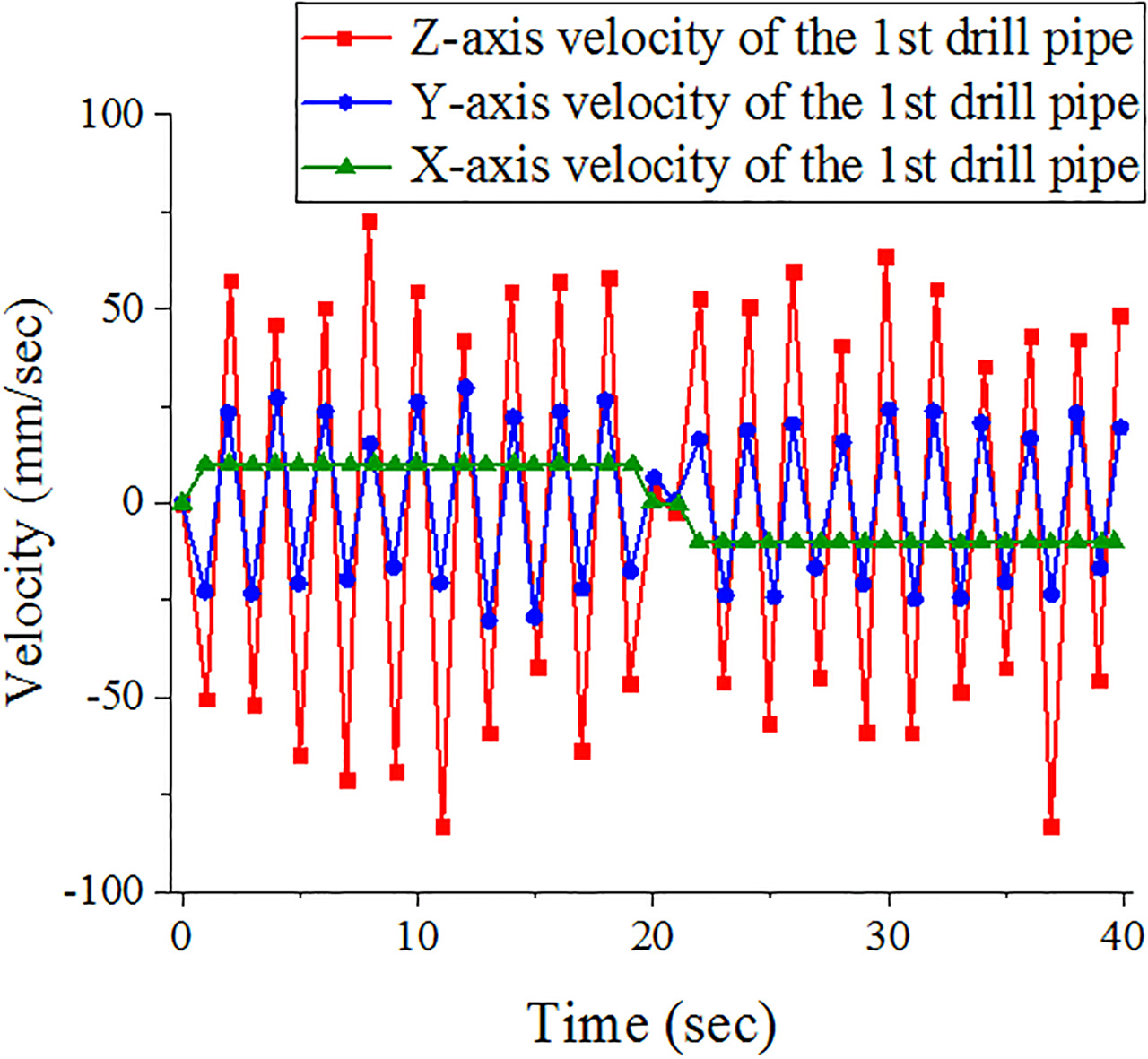

Figure 8.

Z-axis speed of the first, 50th, and 100th drill pipes.

Figure 9.

Displacement of the first drill pipe along Y and Z-axis.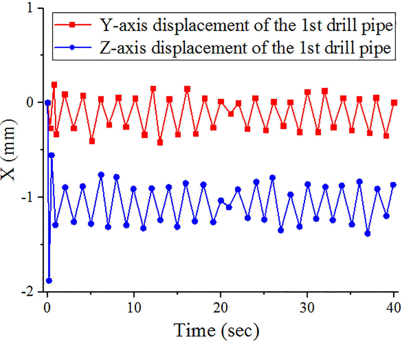

Red line with square symbol (curve 1 ), blue line with circle symbol (curve 2 ), and green line with triangle symbol (curve 3 ) in Fig. 7 are the Z-axis, Y-axis, and X-axis velocity of the 1st drill pipe, respectively. Using curve 3, it can be verified that the written translational motion parameter program is correct. Throughout the whole figure, although the drive provides the speed of the X-axis, the speed of the Z-axis fluctuate the most because the system is affected by various external forces, while the speed fluctuation of the X-axis is the smallest. In order to reduce the probability of borehole failure more efficiently, the speed change in the Z-axis should be analyzed.

Figure 10.

Z-axis displacement of drill pipes 1, 50 and 100.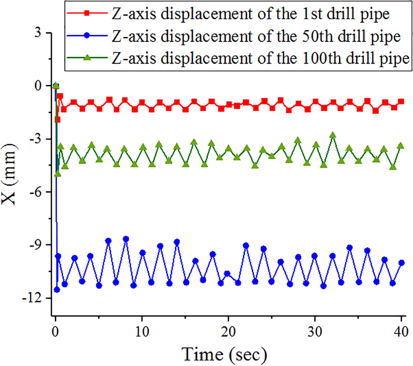

Figure 11.

X-axis displacement amplitude-frequency characteristics in the case of the 100th drill pipe.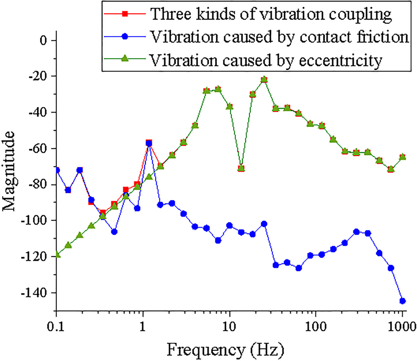

Red line with square symbol (curve 1 ), blue line with circle symbol (curve 2 ), and green line with triangle symbol (curve 3 ) in Fig. 8 are the Z-axis velocity of the 100th drill pipe, the 50th drill pipe and the 1st drill pipe. It can be seen from the figure that the Z-axis velocity of the first rod is least affected by vibration and friction. As the number of rods increases, the amplitude of the curve increases continuously, and the probability of sudden change in amplitude increases, so the jump phenomenon is more likely occurs in the deep hole section.

Red line with square symbol (curve 1 ) in Fig. 9 is the Y-axis displacement of the first drill pipe, and its mean value is $-$ 0.1201 mm. Blue line with circle symbol (curve 2 ) is the Z-axis displacement of the first drill pipe, and its mean value is $-$ 1.0726 mm. Under the action of gravity, the first drill pipe the displacement of the Z-axis is greater than the displacement of the Y-axis. Therefore, the damage of the drill pipe to the lower wall of the Z-axis is more serious, and the amplitude of the Z-axis displacement within 1 s of starting is slightly larger than the amplitude of the Z-axis displacement at the time of stationary.

Figure 10 focuses on the more serious Z-axis displacement, where red line with square symbol (curve 1 ) is the Z-axis displacement of the first drill pipe, the average value is $-$ 1.0726 mm, blue line with circle symbol (curve 2 ) is the Z-axis displacement of the 50th drill pipe, the average value is $-$ 10.5554 mm, green line with triangle symbol (curve 3 ) is the Z-axis displacement of the 100th drill pipe, and the average value is $-$ 3.9166 mm. The first drill pipe is connected to the drive, and the 100th bar is connected to the rigid drill bit. Due to the gravity, the three curves are all negative, the contact force between the 50th drill pipe and the ground is the largest, the lower end of the Z-axis displacement curve fluctuates slightly, showing an upward fluctuation state, and the 50th rod displacement value and fluctuation amplitude are greater than the first drill pipe and the 100th drill pipe.

In Figs 7 and 9, the differences of the three curves are caused by the different directions of the coordinate axes. In Figs 8 and 10, the differences of the three curves are caused by the drilling depth.

Figure 11 is a graph showing the X-axis displacement frequency response of the 100th drill pipe, where red line with square symbol (curve 1 ) takes into account the coupling (coupling vibration) of drive induced excitation (drive vibration), contact friction induced vibration (friction vibration) and eccentric induced vibration (eccentric vibration). blue line with circle symbol (curve 2 ) considers the frictional vibration, and green line with triangle symbol (curve 3 ) considers the eccentric vibration. It can be seen from the figure that the system is more affected by the frictional vibration before 1.58 Hz, and the system is more affected by the eccentric vibration after 1.58 Hz. The coupled vibration curve is more consistent with the frictional vibration curve which has greater influence on the system before 1.58 Hz, and is more consistent with the eccentric vibration curve which has greater influence on the system after 1.58 Hz. Therefore, it is more reasonable to analyze the coupled vibration in all frequency ranges, the subsequent simulation only analyzes the coupled vibration.

Figure 12.

System mode.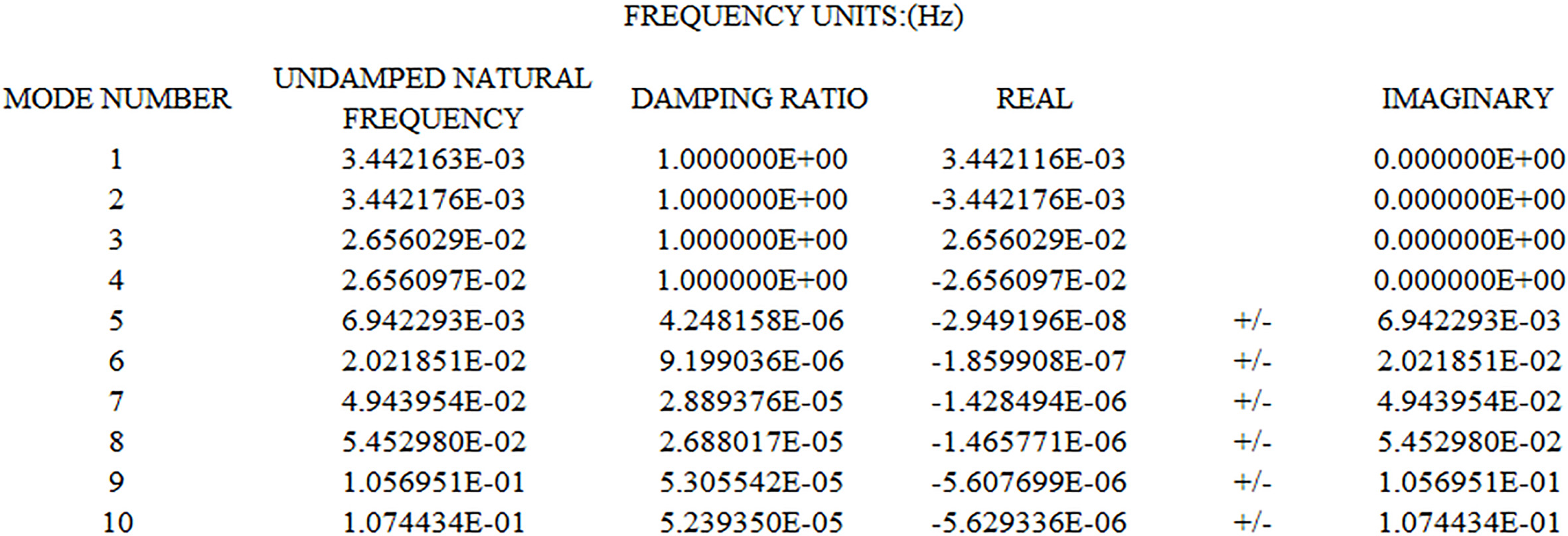

Figure 13.

Modal vibration mode.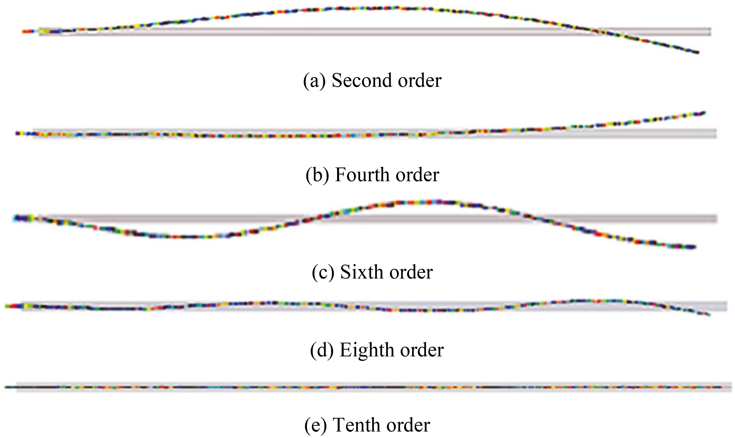

Figure 12 shows the modal data of the system. Corresponding modal data can be seen that there are a total of 2022 order modes in the system. Because it is a rigid-flexible coupling system, and from the eigenvalue table, the damping ratio of the first 4 orders of data is 1 and the imaginary part is 0. The frequency depends only on the real part, which is consistent with the stiffness theory, so the first 4 orders are rigid body modes. The figure only lists the modal frequencies of the first 10 orders that affect the dynamic characteristics of the system. It can be seen from the full 2022 order modal table that the frequency range is 6.9E-3 to 2.1E+4. In practical engineering, the vibration excitation of the driver can be controlled to avoid the modal frequency, reduce the vibration and reduce the probability of borehole failure.

Due to the excessive modality, the second, fourth, sixth, eighth, and tenth modal are selected for analysis. In Fig. 13a–e are the second order, fourth order, sixth order, eighth order, and tenth order Modal Vibration Mode, respectively. It can be seen from the figure that the mode shapes of each mode are different, which is due to the fact that the modes differ by a fixed position angle, that is, the system matrix feature vectors are different.

Figure 14.

The influence of the length of the drill pipe on the natural frequency of the system.

Figure 15.

The influence of the length of each drill pipe on the natural frequencies of the system.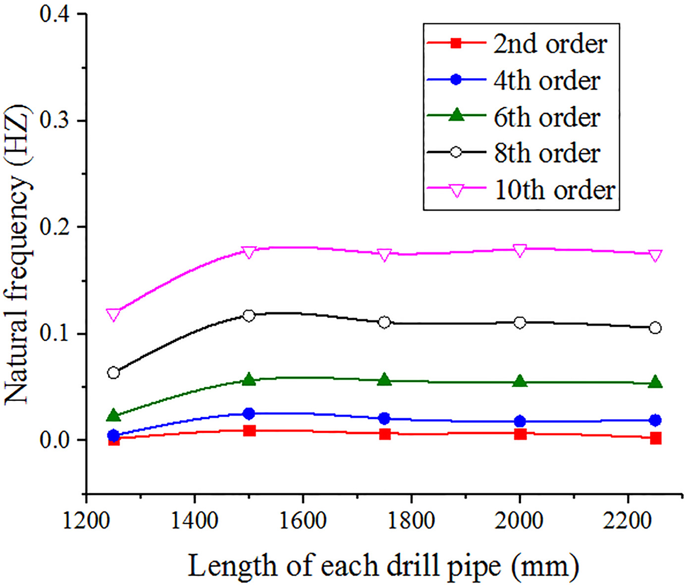

Red line with solid square symbol (curve 1 ), blue line with solid circle symbol (curve 2 ), green line with solid triangle symbol (curve 3 ), black line with hollow circle symbol (curve 4 ), and pink line with hollow triangle symbol (curve 5 ) in Fig. 14 are the second order, fourth order, sixth order, eighth order, and tenth order natural frequency. It can be seen from the figure that when the length of the drill pipe is constant, the natural frequency of the system increases with the increase of the order. When the order is constant, the natural frequency decreases as the drilling length increases. In the shallow hole section, the natural frequency of the system is the largest and the convergence is the fastest. As the depth increases, the convergence speed gradually becomes slower and eventually reaches a certain value. That is, the natural frequency of the shallow hole section is greatly affected by the order number, and the natural frequency of the deep hole section is hardly affected by the order.

In this paper, the correctness of the simulation is verified by referring to the experimental results of “Research on drill pipe vibration characteristics of horizontal directional drilling machine” written by Kong degong of China. In this paper, the equal diameter steel pipe is used to replace the drill pipe as the experimental object, and the natural frequency of the specimen is obtained indirectly by measuring the strain vibration frequency. The results show that the average natural frequency of three experiments is 0.94547 Hz when the length of steel tube is 7 m, 0.64124 Hz when the length of steel tube is 8.5 m, and 0.46330 Hz when the length of steel tube is 10 m. Due to the different parameters, the experimental results are different from those in this paper, but the curve trend is consistent with that in this paper. With the increase of the length, the inherent decreases, the shorter the length, the faster the reduction, and finally tends to be stable. Thus, the simulation results of this paper are correct.

5. Conclusions

In this paper, the Newton-Eulerian method is used to model the rigid body, and the second type of Lagrangian equation is used to model the flexible body. The relative node coordinate method is used to assemble the rigid model and the flexible model, and the finite element method is used. The model is discrete to perform more in-depth calculations on the mathematical model. The model assumes that the materials in the system are all isotropic. In addition, the values of friction coefficient, elastic modulus, Poisson’s ratio and other parameters are not considered.

(1)

Friction and vibration coupling does not necessarily increase the probability of drilling failure, and sometimes it may suppress the amplitude of vibration. Before 1.58 Hz, the system is more affected by frictional vibration (vibration caused by friction). After 1.58 Hz, the system is more affected by eccentric vibration (vibration caused by eccentricity). The coupled vibration (drive-induced excitation, frictional vibration, eccentric vibration coupling) curve is more consistent with the frictional vibration curve which have a greater influence on the system before 1.58 Hz, and it more consistent the eccentric vibration curve which have a greater influence on the system after 1.58 Hz, therefore, it is more reasonable to analyze the coupled vibration in all frequency ranges.

(2)

As the number of rods increases, the Z-axis velocity is continuously affected by vibration and friction, and the probability of abrupt amplitude increases. Therefore, the jumping phenomenon is more likely to occur in the deep hole portion.

(3)

The working frequency range of the drilling rig is 6.9e-3-2.1e+4. Compared with the length of each drill pipe, the influence of drilling depth on the system should be considered. In addition, the natural frequency of shallow hole section is greatly affected by the order, while the natural frequency of deep hole section is less affected by the order. In practical engineering, the mode frequency can be avoided by controlling the vibration excitation of the actuator, thus reducing the vibration and the probability of drilling failure.

(4)

Compared with the traditional finite element method, the multi-body dynamic method is more efficient and more conducive to the optimization calculation. It is very important to use different methods to calculate the rigid body and flexible body, and consider two kinds of coupling (coupling between rigid body and flexible body and coupling between friction and vibration), which will make the analysis results more accurate. The model can simulate a series of dynamic responses of drilling rig system in drilling process, and provide theoretical support for subsequent multi-factor coupling modeling.

Footnotes

Acknowledgments

This work was support by the National Natural Science Foundation of China (Nos. 51275061 and 61672121), the Scientific Research Project of Lingnan Normal University (No. ZL2025). The authors would also like to express sincere appreciation to the anonymous reviewers for their insightful comments and suggestions on an earlier draft of this paper.

References

Bradley

W.B.

, Failure of inclined boreholes, Journal of Energy Resources Technology 101(4) (1979), 232–239.

Gupta

and Zaman

, Stability of boreholes in a geologic medium including the effects of anisotropy, Applied Mathematics and Mechanics 20(8) (1999), 837–866.

Yuan

J.L.

et al., Borehole stability analysis of horizontal drilling in shale gas reservoirs, Rock Mechanics and Rock Engineering 46(5) (2013), 1157–1164.

Lan

H.T.

and Moore

I.D.

, Numerical investigation of the circumferential stresses around boreholes during horizontal directional drilling, International Journal of Geomechanics 17(12) (2017), 04017114.

Cheng

et al., Numerical simulation for the dynamic breakout of a borehole using boundary element method, Geotechnical and Geological Engineering 37(4) (2019), 2873–2881.

et al., Elastic-softening-plasticity around a borehole: an analytical and experimental study, Rock Mechanics & Rock Engineering 52(4) (2019), 1149–1164.

Zhang

H.Y.

et al., Effect of fluid temperature on rock failure in borehole drilling, Journal of Engineering Mechanics 140(1) (2014), 82–90.

Tian

J.L.

et al., Study on lateral vibration characteristics of a drill string with transverse inertia effect, Journal of Failure Analysis and Prevention 16(4) (2016), 678-682.

Rahimi

and Nygaard

, Effect of rock strength variation on the estimated borehole breakout using shear failure criteria, Geomechanics and Geophysics for Geo-energy and Geo-resources 4(4) (2018), 369–382.

10.

Lobo

D.M.

Ritto

T.G.

and Castello

D.A.

, Stochastic analysis of torsional drill-string vibrations considering the passage from a soft to a harder rock layer, Journal of the Brazilian Society of Mechanical Sciences and Engineering 39(6) (2017), 2341–2349.

11.

Cheng

Z.B.

et al., A multibody dynamical model for full hole drillstring dynamics, Applied Mechanics and Materials 378 (2013), 91–96.

12.

Belyaev

A.K.

and Eliseev

V.V.

, Flexible rod model for the rotation of a drill string in an arbitrary borehole, Acta Mechanica 229(2) (2018), 841–848.

13.

Tan

L.C.

et al., Casing wear prediction model based on drill string whirling motion in extended-reach drilling, Arabian Journal for Science and Engineering 43(11) (2018), 6325–6332.

14.

Kapitaniaka

et al., Unveiling complexity of drill-string vibrations: Experiments and modelling, International Journal of Mechanical Sciences 101-102 (2015), 324–337.

15.

Tang

L.P.

Zhu

X.H.

and Li

J.H.

, Effects of the synchronous variation of the static and the kinetic friction coefficients on stick-slip vibration of drillstring, Iranian Journal of Science and Technology, Transactions of Mechanical Engineering 43(Supplement 1) (2019), 275–283.

16.

Nogueira

B.F.

and Ritto

T.G.

, Stochastic torsional stability of an oil drill-string, Meccanica 53(11–12) (2018), 3047–3060.

17.

Divenyi

et al., Drill-string vibration analysis using non-smooth dynamics approach, Nonlinear Dynamics 70(2) (2012), 1017–1035.

18.

Melakhessou

Berlioz

and Ferraris

, A Nonlinear Well-Drillstring Interaction Model, Journal of Vibration and Acoustics 125(1) (2003), 46–52.

19.

García-Vallejo

et al., Describing Rigid-Flexible Multibody Systems Using Absolute Coordinates, Nonlinear Dynamics 34(1–2) (2003), 75–94.

20.

Arbatani

et al., An approach to directional drilling simulation: finite element and finite segment methods with contact, Computational Mechanics 57(6) (2016), 1001–1015.

21.

Liang

Y.T.

and McPhee

, Symbolic integration of multibody system dynamics with the finite element method, Multibody System Dynamics 43(4) (2018), 387–405.

22.

Sun

and Fish

, Superposition-based coupling of peridynamics and finite element method, Computational Mechanics 64(1) (2019), 231–248.

23.

Verdugo

Martín

A.F.

and Badia

, Distributed-memory parallelization of the aggregated unfitted finite element method, Computer Methods in Applied Mechanics and Engineering 357 (2019), 112583.

24.

Kim

et al., Flexible multibody dynamics using coordinate reduction improved by dynamic correction, Multibody System Dynamics 42(4) (2018), 411–429.

25.

Wang

Tian

and Hu

H.Y.

, Multiple dynamic response patterns of flexible multibody systems with random uncertain parameters, Journal of Computational and Nonlinear Dynamics 14(2) (2019), 021008.

26.

Daocharoenporn

et al., Prediction of the Pantograph/Catenary Wear Using Nonlinear Multibody System Dynamic Algorithms, Journal of Tribology 141(5) (2019), 051603.

27.

Charles

Casenave

and Glocker

, A catching-up algorithm for multibody dynamics with impacts and dry friction, Computer Methods in Applied Mechanics & Engineering 334 (2018), 208–237.

28.

Sui

and Ding

, Numerical Analysis of Dry Friction – Induced Vibration of Moving Slider – Elastic Annular Beam System, Transactions of Nanjing University of Aeronautics and Astronautics 35(1) (2018), 84–93.