QSPR prediction of polymers’ solubility parameters by radial basis functional link net

Abstract

This research aims to introduce a novel radial basis functional link net (RBFLN)-based QSPR (quantitative structure-property relationship) model to predict the solubility parameters of the polymers with the structure – (C ${}^{1}$ H ${}_{2}--$ C ${}^{2}$ R ${}^{3}$ R ${}^{4}$ ) – and provides its comparison with the multi-layer feed forward network (MLFFN)-based QSPR model, as well as previous genetic programming (GP) and multiple linear regression (MLR)-based QSPR models in the literature. During the implementation of the RBFLN and MLFFN-based QSPR models, the networks which are associated with the minimum weighted average AIC (Akaike’s information criterion) and BIC (Bayesian information criterion) scores are trained by using a hybrid scheme combining the cuckoo search and Levenberg-Marquardt algorithm. Our results show that the RBFLN-based QSPR model outperforms the other ones in terms of the external validation metrics. The study also reveals that it may have a promising potential to study the relationship between various measurement/experimental data or processing elements in a hybrid way of artificial intelligence modelling.

Keywords

Polymer solubility neural networks radial basis functional link net QSPR cuckoo searchArticle Highlights:•The RBFLN based QSPR model accurately predicts the solubility parameters.•The RBFLN is able to provide a much simpler solution than the MLFFN.•The hybridization of CS and LM algorithms is an effective training strategy.

1. Introduction

Until today, a few researchers have used QSPR (quantitative structure-property relationship) modelling [1] for the prediction of the solubility parameters of polymers: Yu et al. [2] constructed a QSPR model correlating the solubility parameters of polymers with their molecular structures by using common multiple linear regression. Goudarzi et al. [3] and Koç and Koç [4] demonstrated the applicability of different artificial intelligence tools (i.e., genetic programming and least square support vector machine) on the same problem but with different data sets of training and testing, and they consequently reported that their predictive performances were better than the traditional multiple linear regressions. However, this research subject is still in its preliminary stages and needs further investigation to know the relative merits of many other different ways of artificial intelligence-based modelling. This has motivated the present study exploring the radial basis functional link net or network (RBFLN) as an alternate artificial intelligence-based model for the solubility prediction of polymers. It is a hybrid model [5] combining the functional link net [6] with the radial basis functions [7], which achieves faster convergence and more accuracy than the widely-used multilayer feed forward network [5]. Both networks have formally same structure where Levenberg-Marquardt algorithm is widely used as one of the most efficient training methods due to its fast convergence and high accuracy [8, 9, 10, 11, 12, 13]. On the other hand, this type of iterative local optimization strongly requires a “good” initialization close to the global optimum to avoid falling into a local optimum, and many empirical findings have suggested that a global search method (e.g., cuckoo search) is able to easily find a good initial estimate of the optimum solution which is then refined by the Levenberg-Marquardt algorithm [14, 15, 16]. Cuckoo search is a relatively new meta-heuristic algorithm [17, 18] based on the brood parasitism of some cuckoo species, which is potentially more powerful than many other optimization techniques [14, 19, 20]. Considering the points mentioned above, this study primarily proposes a novel QSPR modelling method based on the radial basis functional link network (i.e. called RBFLN-QSPR) which uses a hybrid learning scheme combining the cuckoo search and Levenberg-Marquardt algorithm, and then applies it to predict the solubility of polymers. One recent literature survey showed that the RBFLN received little attention [21, 22, 23, 24, 25] but there was no any research about QSPR modelling using the RBFLN.

The RBFLN-QSPR is implemented using five steps for better clarity and ease of use, and its predictive performance is compared to that of multilayer feed forward network (MLFFN)-based QSPR model (MLFFN-QSPR) in order to evaluate its predictive capability. The results of internal (goodness of fit) and external validation (testing) of these models are also compared to the results of previously-developed models that are known as the genetic programming-based QSPR model (GP-QSPR) and the multiple linear regression-based QSPR model (MLR-QSPR) [4]. It must be noted here that these QSPR models received the same training and testing data sets [4] including the experimental solubility parameters and molecular descriptors of 97 polymers with the structure – (C ${}^{1}$ H ${}_{2}$ –C ${}^{2}$ R ${}^{3}$ R ${}^{4}$ ) – [2], during their learning and testing stages. This implies that this study provides a unifying view that evaluates all of the above-mentioned models in a QSPR study.

The remainder of the paper is organized as follows: Section 2 is devoted to the theoretical description of the neural network models (RBFLN and MLFNN). Section 3 presents the details of the implementations with the results and discussion heading. Finally, concluding remarks are given in Section 4.

2. Theory and calculation

RBFLN (Fig. 1) is formally similar to three-layered MLFFN (Fig. 2) but has extra connectivity from the input to the output layer [21, 24]. Thus, each of $z$ output layer neurons receives weighted inputs from each of $s$ neurons of Gaussian hidden layer as well as $k$ neurons of input layer that allows a more complete model of a general non-linear mapping between input and output pairs [5, 25], as shown below:

$\displaystyle Y=(W_{e}X+W_{o}^{T}\phi)$ (1)

Figure 1.

RBFLN model.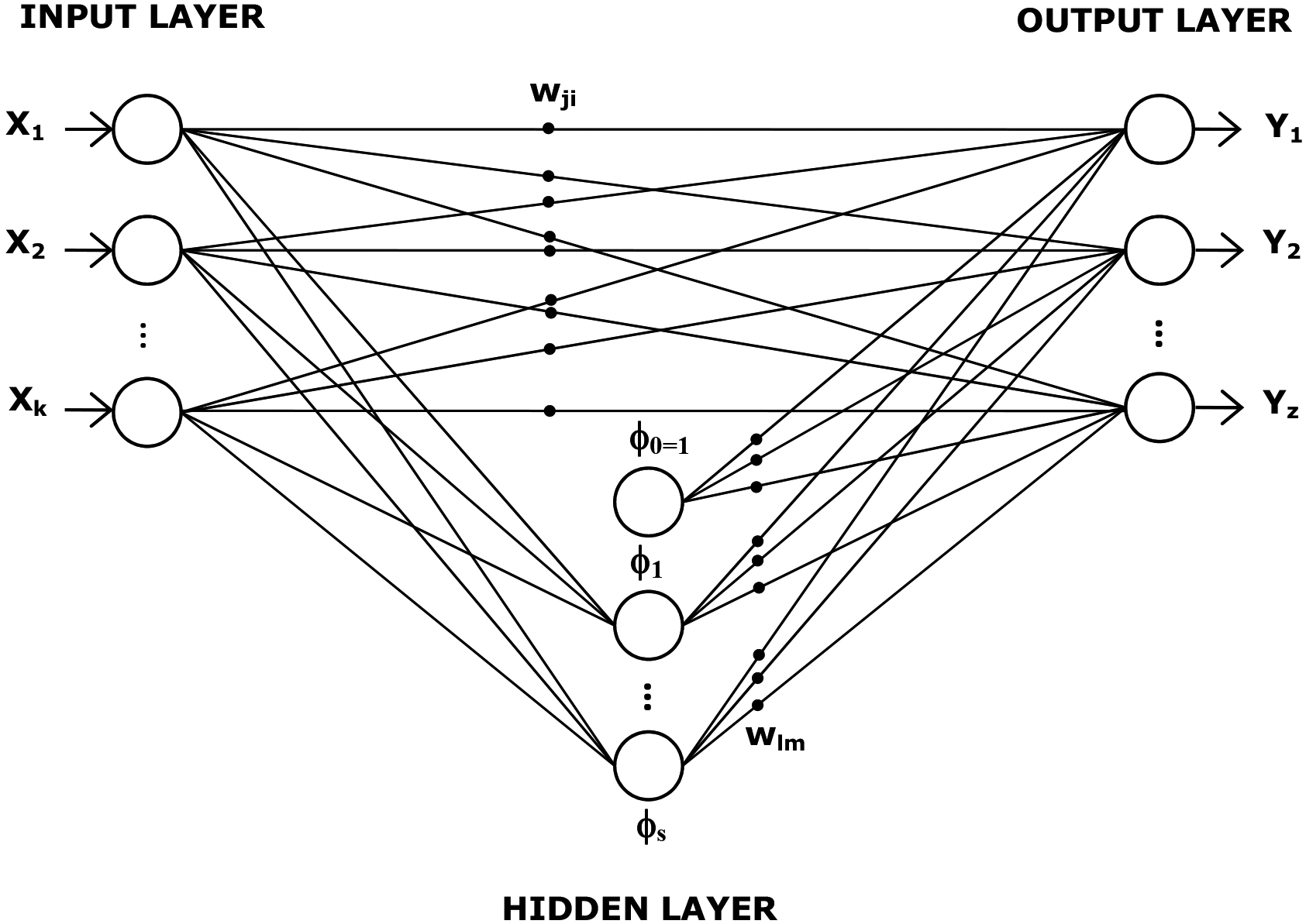

Figure 2.

MLFFN model.

where $Y$ is the output matrix with the component $y_{ji}\left({j=1,\ldots,z;i=1,\ldots,N}\right)$ , $X$ is the input matrix with the component $x_{ji}\left({j=1,\ldots,k;i=1,\ldots,N}\right)$ , $W_{e}$ denotes the input-output layer or extra weight matrix with the component $w_{ji}\left({j=1,\ldots,z;i=1,\ldots,k}\right)$ , $W_{o}$ denotes the hidden-output layer weight matrix with the component $w_{lm}\left({l=1,\ldots,s;m=1,\ldots,z}\right)$ , $\phi$ is the hidden layer output matrix with the component $\phi_{rp}=\exp\left({-\beta_{r}||x_{p}-c_{r}||^{2}}\right)\left({r=1,\ldots,s;% p=1,\ldots,N}\right)$ which is the output of the $r^{\text{th}}$ neuron for the $p^{\text{th}}$ sample from the Gaussian function characterized by the prototype vector $c_{r}$ and the spread parameter $\beta_{r}$ and $x_{p}=\left[{x_{1p},x_{2p},\ldots,x_{kp}}\right]^{T}$ is the input vector ( $p=1,\ldots,N$ ).

MLFFN model [7, 8, 26], unlike RBFLN, has different non-linear transfer functions (e.g., sigmoid, hyperbolic tangent) which can be used for hidden and output layers:

$\displaystyle Y=\varphi\left({W_{o}^{T}\left({(\psi\left({W_{h}X}\right)}% \right)}\right)$ (2)

where $W_{h}$ denotes the input-hidden layer weight matrix with the component $w_{ji}(j=1,\ldots,s;i=1,\ldots,\linebreak k)$ , also $\psi$ and $\varphi$ are the transfer functions in the hidden and output layers, respectively.

Using the Levenberg-Marquardt (LM) training algorithm based on the minimization of objective function $F\left(w\right)=e^{T}e$ , the vector $\left(w\right)$ of network parameters (i.e., connection weights, prototype vectors and spread parameters) at the iteration step $t$ can be modified as follows [27, 28, 29, 30]:

$\displaystyle w_{t+1}=w-\left({J^{T}\left(w\right)J\left(w\right)+\mu I}\right% )^{-1}J^{T}\left(w\right)e\left(w\right)$ (3)

where $e\left(w\right)$ is the error vector, $J\left(w\right)$ is the Jacobian matrix, $I$ is the identity matrix, $\mu$ is the learning parameter, $w_{t+1}$ represents the updated vector of network parameters at the iteration step $\left({t+1}\right)$ , and the vector of network parameters can be initialized with the cuckoo search (CS) algorithm which simulates the aggressive reproduction strategy of cuckoo birds on the basis of three main rules [17, 18]: 1) Each cuckoo lays one egg at a time in a randomly chosen nest, 2) The best nests with high-quality eggs or solutions will be carried over to the next generations, 3) The number of available host nests is constant, and a host bird can discover an alien egg with a probability $p_{a}\in\left[{0,1}\right]$ . The pseudo-code of the CS algorithm used in this study is given as follows:

Generate initial population of $n$ host nests $w_{i}$ which consists of parameters (i.e., weights, prototype vectors and spread parameters) of the networks and finds the fitness $F_{i}$ value by using the objective function $\left({i=1,\ldots,n}\right)$ . While (Stop criterion) Get a cuckoo (say $j$ ) randomly by the Lévy flight with the step size $\alpha$ and evaluate its fitness $F_{j}$ by using the objective function Choose a nest $i$ among $n$ randomly if $F_{j}>F_{i}$ then $w_{i}\leftarrow w_{j}$ $F_{i}\leftarrow F_{j}$ end if A fraction ( $P_{a}$ ) of worse nests are abandoned and new ones are built by the Lévy flight Evaluate the fitness of new nests by using the objective function Keep the best solutions/nests Rank the solutions and find the current best end while

where the Lévy flight is a type of random walk which is characterized by a series of consecutive jump steps drawn from the Lévy distribution [17]. When exploring new solutions, the scale of flight is controlled by a step size factor $\alpha>0$ . In this study, the various parameters involved in the CS and LM algorithms were selected as follows: The number of nests $\left(n\right)$ was set to 25. The step size factor $\alpha$ and discovery probability $\left({p_{a}}\right)$ were adjusted at 0.01 and 0.25, respectively. As the stop criterion, the maximum number of generation was set to 500. The initial value of the learning parameter $\left(\mu\right)$ was taken as 0.001.

3. Results and discussion

RBFLN-QSPR and MLFFN-QSPR models were implemented step by step (Fig. 3) as follows.

In step i, the input $\left({x=\left[{hb,\textit{alk},n_{N},Q_{ii},E_{\textit{int}},Q_{H}}\right]^{T% }}\right)$ and output $\left({y=\left[\delta\right]}\right)$ vectors of the networks were chosen based on our previous study [4], where $\delta$ is the solubility parameter in $(\text{J}/cc)^{0.5}$ , $hb=\frac{mQ_{\pm}}{n^{2}}$ , $m$ is the number of –OH, –NH or –CN group in the side groups, $Q_{\pm}$ is the hydrogen bond descriptor, $n$ is the number of atoms from the terminal atom in the constituent group R ${}^{3}$ or R ${}^{4}$ to the atom C ${}^{2}$ , alk is a descriptor which is used to judge whether a polymer belongs to polyalkenes or not, $n_{N}$ is the number of nitrogen atoms in repeating units, $Q_{ii}$ is the quadrupole moment (Debye Å), $E_{\textit{int}}$ is the thermal energy (4.19 $\times$ 10 ${}^{9}$ J/mol) and $Q_{H}$ is the most positive charge of a hydrogen atom (a.u). The details on the calculation and selection of descriptors are presented completely by Yu et al. in [2].

In step ii, the input and output data were normalized within the range of $-$ 1 to 1, as follows: $x=\left[{\frac{hb}{\max\left({\left|{hb}\right|}\right)},\frac{\textit{alk}}{% \max\left({\left|{\textit{alk}}\right|}\right)},\frac{n_{N}}{\max\left({\left|% {n_{N}}\right|}\right)},\frac{Q_{ii}}{\max\left({\left|{Q_{ii}}\right|}\right)% },\frac{E_{\textit{int}}}{\max\left({\left|{E_{\textit{int}}}\right|}\right)},% \frac{Q_{H}}{\max\left({\left|{Q_{H}}\right|}\right)}}\right]^{T}$ and $y=\left[{\frac{\delta}{\max\left({\left|\delta\right|}\right)}}\right]$ . The ranges of variables of randomly-selected training and testing data sets (Tables 3 and 4) [4] are given in Tables 1 and 2, respectively.

Table 1
Ranges of inputs and output ( $\delta$ ) variables in the training data set [4]

Variable	Minimum (40 data samples)	Maximum (40 data samples)
$h b$	$-$ 0.0483	0
alk	0	1
$n_{N}$	0	1
$Q_{ii}$ (Debye Å)	$-$ 90.1358	$-$ 18.9995
$E_{\textit{int}}$ (4.19 $\times$ 10 ${}^{9}$ J/mol)	36.9640	229.0590
$Q_{H}$ (a.u.)	0.1259	0.4075
$\delta$ (J/cc) ${}^{0.5}$	16.00	31.00

Figure 3.

The flowchart of the RBFLN- and MLFFN-based QSPR modelling steps.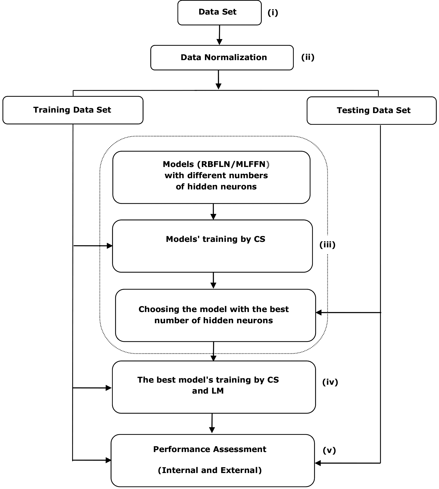

Table 2

Ranges of inputs and output ( $\delta$ ) variables in the testing data set [4]

Variable	Minimum (57 data samples)	Maximum (57 data samples)
$h b$	$-$ 0.0173	0
alk	0	1
$n_{N}$	0	1
$Q_{ii}$ (Debye Å)	$-$ 83.9006	$-$ 14.8853
$E_{\textit{int}}$ (4.19 $\times$ 10 ${}^{9}$ J/mol)	39.3470	210.6090
$Q_{H}$ (a.u.)	0.1332	0.2365
$\delta$ (J/cc) ${}^{0.5}$	16.80	25.90

Table 3

Experimental solubility parameters and calculated molecular descriptors [2] comprising the training data set [4]

No	Polymers	$h b$	alk	$n_{N}$	$Q_{ii}$ (Debye Å)	$E_{\textit{int}}$ (4.19 $\times$ 10 ${}^{9}$ J/mol)		$Q_{H}$ (a.u.)	$\delta$ (J/cc) ${}^{0.5}$
1	poly (vinyl alcohol)	$-$ 0.0483	0	0	$-$ 18.9995	53.	080	0.389411	31.00
2	poly (vinyl ethyl ether)	0.0000	0	0	$-$ 32.1344	90.	549	0.157379	17.40
3	poly (vinyl n-butyl ether)	0.0000	0	0	$-$ 45.3354	128.	148	0.157283	17.40
4	poly (methyl acrylate)	0.0000	0	0	$-$ 35.3226	79.	391	0.169044	21.40
5	poly (vinylide bromide)	0.0000	0	0	$-$ 48.5852	38.	757	0.225322	22.80
6	Polyacrylonitrile	$-$ 0.0173	0	1	$-$ 25.8884	49.	879	0.195491	27.50
7	poly (methyl methacrylate)	0.0000	0	0	$-$ 42.0122	98.	081	0.169770	20.20
8	Polymethacrylonitrile	$-$ 0.0173	0	1	$-$ 32.9640	68.	458	0.169271	24.50
9	poly (cyclohexyl methacrylate)	0.0000	0	0	$-$ 67.5836	159.	418	0.170439	19.80
10	poly (benzyl methacrylate)	0.0000	0	0	$-$ 75.1338	151.	847	0.171913	20.70
11	poly (n-octyl methacrylate)	0.0000	0	0	$-$ 90.1358	229.	059	0.168645	18.60
12	poly ( $\alpha$ -vinyl naphthalene)	0.0000	0	0	$-$ 67.7182	134.	601	0.153432	20.90
13	Polyisobutylene	0.0000	1	0	$-$ 27.6679	81.	980	0.196383	16.00
14	poly (1-butene)	0.0000	1	0	$-$ 28.2546	86.	964	0.141067	17.10
15	poly (4-methyl-1-pentene)	0.0000	1	0	$-$ 41.6106	124.	335	0.142244	16.80
16	poly (1,2-butadiene)	0.0000	1	0	$-$ 26.3875	71.	702	0.143982	17.20
17	poly (t-butyl methacrylate)	0.0000	0	0	$-$ 61.6507	152.	874	0.168645	18.30
18	poly (vinyl sec-butyl ether)	0.0000	0	0	$-$ 45.4648	127.	823	0.156900	17.00
19	poly (acrylic acid)	$-$ 0.0121	0	0	$-$ 29.4530	60.	651	0.407577	25.70
20	Polyacrylamide	$-$ 0.0128	0	1	$-$ 29.5498	68.	445	0.338456	28.10
21	poly (vinyl butyrate)	0.0000	0	0	$-$ 48.3401	116.	916	0.174955	18.33
22	poly (vinyl methyl sulfide)	0.0000	0	0	$-$ 33.1509	69.	903	0.182660	19.52
23	poly (vinyl methyl ether)	0.0000	0	0	$-$ 25.7032	71.	814	0.158178	19.66
24	poly (1-ethyl vinyl ethyl ether)	0.0000	0	0	$-$ 45.4476	127.	805	0.163138	19.21
25	poly (vinyl ethyl ketone)	0.0000	0	0	$-$ 38.0354	93.	956	0.160771	22.14
26	poly (4-hydroxystyrene)	$-$ 0.0019	0	0	$-$ 51.4885	106.	037	0.405212	24.55
27	poly (divinyl ether)	0.0000	0	0	$-$ 30.7963	74.	624	0.164267	18.93
28	poly (vinyl-1-phenyl methyl ether)	0.0000	0	0	$-$ 57.2652	125.	420	0.125940	20.17
29	poly (nitro styrene)	0.0000	0	1	$-$ 66.0630	106.	629	0.181215	22.71
30	poly (benzyl acrylate)	0.0000	0	0	$-$ 68.6248	132.	557	0.173749	19.38
31	poly (o-methyl styrene)	0.0000	0	0	$-$ 53.6503	121.	882	0.161500	19.33
32	poly (allyl isocyanide)	$-$ 0.0077	0	1	$-$ 33.0703	68.	590	0.180890	25.45
33	poly (isopropyl methacrylate)	0.0000	0	0	$-$ 55.2181	135.	204	0.173121	18.39
34	poly (allyl isopropyl ether)	0.0000	0	0	$-$ 45.4556	127.	799	0.165117	19.21
35	poly (allyl acetate)	0.0000	0	0	$-$ 42.6179	98.	039	0.181694	18.27
36	poly (propyl methacrylate)	0.0000	0	0	$-$ 55.2974	135.	592	0.164884	18.37
37	poly (3-chloropylpropyl methacrylate)	0.0000	0	0	$-$ 71.2170	130.	324	0.195761	19.60
38	poly (4-acetoxy styrene)	0.0000	0	0	$-$ 67.1294	131.	974	0.185200	21.70
39	poly (vinyl methyl ketone)	0.0000	0	0	$-$ 32.4567	74.	479	0.179187	22.92
40	poly (vinyl-1-amyl methyl ether)	0.0000	0	0	$-$ 60.5029	165.	748	0.155492	20.83

Table 4

Experimental solubility parameters and calculated molecular descriptors [2] comprising the testing data set [4]

No	Polymers	$h b$	alk	$n_{N}$	$Q_{ii}$ (Debye Å)	$E_{\textit{int}}$ (4.19 $\times$ 10 ${}^{9}$ J/mol)	$Q_{H}$ (a.u.)	$\delta$ (J/cc) ${}^{0.5}$
1	Polyethylene	0.0000	1	0	$-$ 14.8853	49.390	0.144396	17.50
2	poly (vinyl chloride)	0.0000	0	0	$-$ 26.1104	44.649	0.193699	21.20
3	poly (vinyl bromide)	0.0000	0	0	$-$ 30.9478	44.301	0.189865	21.10
4	poly (vinyl acetate)	0.0000	0	0	$-$ 37.5420	79.081	0.187471	21.00
5	poly (N-vinyl pyrrolidone)	0.0000	0	1	$-$ 49.4005	110.814	0.185949	22.30
6	poly (vinyl propionate)	0.0000	0	0	$-$ 42.0187	98.073	0.171231	20.40
7	poly (p-t-butyl styrene)	0.0000	0	0	$-$ 73.1496	177.764	0.150444	18.30
8	Polypropylene	0.0000	1	0	$-$ 21.5668	68.170	0.141027	16.80
9	poly (vinyl cyclohexane)	0.0000	0	0	$-$ 53.2023	148.496	0.133253	18.80
10	poly (p-vinyl pyridine)	0.0000	0	1	$-$ 48.2670	96.003	0.153451	22.40
11	poly (vinylidene chloride)	0.0000	0	0	$-$ 38.0945	39.347	0.236595	22.80
12	poly (ethyl acrylate)	0.0000	0	0	$-$ 42.0185	98.080	0.171261	20.50
13	poly (n-butyl acrylate)	0.0000	0	0	$-$ 55.7523	135.730	0.171100	19.70
14	poly (n-butyl methacrylate)	0.0000	0	0	$-$ 62.0600	153.878	0.169082	19.10
15	poly (methyl $\alpha$ -cyanoacrylate)	$-$ 0.0173	0	1	$-$ 49.3941	79.472	0.202023	25.90
16	poly (sec-butyl methacrylate)	0.0000	0	0	$-$ 61.9267	154.070	0.172628	18.80
17	poly (isobutyl methacrylate)	0.0000	0	0	$-$ 62.3509	154.108	0.163776	18.80
18	Polystyrene	0.0000	0	0	$-$ 46.9407	103.346	0.151529	20.10
19	poly (p-methyl styrene)	0.0000	0	0	$-$ 53.1736	121.827	0.159854	19.40
20	poly (p-chloro styrene)	0.0000	0	0	$-$ 59.8069	97.483	0.155354	21.20
21	poly (o-chloro styrene)	0.0000	0	0	$-$ 64.0734	98.119	0.167444	21.20
22	poly (p-bromo styrene)	0.0000	0	0	$-$ 64.0734	97.991	0.155541	21.30
23	poly (ethyl methacrylate)	0.0000	0	0	$-$ 48.6274	116.764	0.164616	19.60
24	poly ( $\alpha$ -methyl styrene)	0.0000	0	0	$-$ 53.7554	121.931	0.149414	19.30
25	poly (n-propyl acrylate)	0.0000	0	0	$-$ 48.7428	116.904	0.171168	20.00
26	poly (n-hexyl methacrylate)	0.0000	0	0	$-$ 76.0284	191.485	0.169107	18.80
27	poly (N-vinyl carbazole)	0.0000	0	1	$-$ 83.3121	154.192	0.163543	21.60
28	poly (ethyl $\alpha$ -chloroacrylate)	0.0000	0	0	$-$ 53.7529	93.038	0.208716	21.50
29	poly (p-fluoro styrene)	0.0000	0	0	$-$ 52.0063	98.161	0.152659	20.00
30	poly (isobutyl acrylate)	0.0000	0	0	$-$ 57.5115	135.272	0.175174	19.40
31	poly (2-ethoxyethyl methacrylate)	0.0000	0	0	$-$ 65.8952	157.397	0.170405	19.20
32	poly (vinyl phenyl ether)	0.0000	0	0	$-$ 51.1778	106.834	0.163371	20.19
33	poly (m-methyl styrene)	0.0000	0	0	$-$ 53.2890	121.184	0.160541	19.33
34	poly (methoxy styrene)	0.0000	0	0	$-$ 57.4224	125.550	0.167221	20.19
35	poly (1-methyl vinyl ethyl ether)	0.0000	0	0	$-$ 38.8704	108.994	0.157001	19.29
36	poly (1-phenyl vinyl ethyl ether)	0.0000	0	0	$-$ 63.8969	144.154	0.159666	20.03
37	poly (1,1-diphenyl ethylene)	0.0000	0	0	$-$ 79.4181	157.147	0.151710	19.93
38	poly (allyl 4,tolyl ether)	0.0000	0	0	$-$ 63.9397	144.110	0.158223	20.03
39	poly (allyl cyanide)	$-$ 0.0077	0	1	$-$ 34.0233	68.638	0.190630	25.45
40	poly (vinyl phenyl sulfide)	0.0000	0	0	$-$ 58.5896	105.160	0.178789	20.28
41	poly (vinyl propyl ether)	0.0000	0	0	$-$ 38.7548	109.372	0.157346	19.29
42	poly (vinyl isopropyl ether)	0.0000	0	0	$-$ 38.8705	108.993	0.157011	19.29
43	poly (vinyl isoamyl ether)	0.0000	0	0	$-$ 52.1351	146.684	0.157383	19.13
44	poly (vinyl-1-methyl phenyl ether)	0.0000	0	0	$-$ 57.9679	125.272	0.160936	20.19
45	poly (vinyl-1-phenyl phenyl ether)	0.0000	0	0	$-$ 83.9006	160.406	0.162306	20.50
46	poly (2-nitro styrene)	0.0000	0	1	$-$ 63.9986	106.664	0.182582	22.20
47	poly (vinyl isobutyl ether)	0.0000	0	0	$-$ 45.2702	127.889	0.157283	19.21
48	poly (2-ethyl hexyl acrylate)	0.0000	0	0	$-$ 83.3478	210.609	0.171944	18.45
49	poly (allyl phenyl ether)	0.0000	0	0	$-$ 57.9832	125.686	0.153756	20.19
50	poly (allyl methyl ether)	0.0000	0	0	$-$ 32.1471	90.652	0.156307	19.44
51	poly (allyl ethyl ether)	0.0000	0	0	$-$ 38.6678	109.369	0.157454	19.28
52	poly (allyl propyl ether)	0.0000	0	0	$-$ 45.3318	128.193	0.149001	19.21

Table 4, continued
No	Polymers	$h b$	alk	$n_{N}$	$Q_{ii}$ (Debye Å)	$E_{\textit{int}}$ (4.19 $\times$ 10 ${}^{9}$ J/mol)	$Q_{H}$ (a.u.)	$\delta$ (J/cc) ${}^{0.5}$
53	poly (diallyl ether)	0.0000	0	0	$-$ 43.5797	112.800	0.149843	18.84
54	poly (allyl 2, tolyl ether)	0.0000	0	0	$-$ 64.3572	143.642	0.177444	20.03
55	poly (allyl 3, tolyl ether)	0.0000	0	0	$-$ 63.8511	143.549	0.161917	20.03
56	poly (allyl acetonitrile)	$-$ 0.0043	0	1	$-$ 41.9580	87.485	0.190713	24.18
57	poly (cyano styrene)	$-$ 0.0019	0	1	$-$ 62.9157	103.633	0.161041	22.36

Table 5

The result of experiments for RBFLN-based QSPR model

$s$	$m$	$\textit{AIC}_{tr}$	$\textit{BIC}_{tr}$	$\textit{AIC}_{ts}$	$\textit{BIC}_{ts}$	$\overline{\textit{AIC}}$	$\overline{\textit{BIC}}$
1	15	$-$ 5.905	$-$ 5.790	$-$ 7.324	$-$ 7.227	$-$ 6.739	$-$ 6.635
2	23	$-$ 5.930	$-$ 5.797	$-$ 6.623	$-$ 6.511	$-$ 6.337	$-$ 6.216
3	31	$-$ 5.889	$-$ 5.744	$-$ 5.762	$-$ 5.638	$-$ 5.814	$-$ 5.682
4	39	$-$ 5.884	$-$ 5.729	$-$ 5.729	$-$ 6.598	$-$ 6.381	$-$ 6.240
5	47	$-$ 5.874	$-$ 5.711	$-$ 6.477	$-$ 6.339	$-$ 6.228	$-$ 6.080
6	55	$-$ 5.670	$-$ 5.501	$-$ 6.430	$-$ 6.287	$-$ 6.117	$-$ 5.963

Table 6

The result of experiments for MLFFN-based QSPR model

$s$	$m$	$\textit{AIC}_{tr}$	$\textit{BIC}_{tr}$	$\textit{AIC}_{ts}$	$\textit{BIC}_{ts}$	$\overline{\textit{AIC}}$	$\overline{\textit{BIC}}$
1	9	$-$ 5.884	$-$ 5.791	$-$ 6.860	$-$ 6.782	$-$ 6.458	$-$ 6.373
2	17	$-$ 5.886	$-$ 5.766	$-$ 7.192	$-$ 7.090	$-$ 6.653	$-$ 6.544
3	25	$-$ 5.856	$-$ 5.720	$-$ 7.046	$-$ 6.931	$-$ 6.555	$-$ 6.431
4	33	$-$ 5.818	$-$ 5.670	$-$ 6.811	$-$ 6.685	$-$ 6.401	$-$ 6.267
5	41	$-$ 5.899	$-$ 5.742	$-$ 7.656	$-$ 7.523	$-$ 6.932	$-$ 6.789
6	49	$-$ 5.801	$-$ 5.637	$-$ 7.911	$-$ 7.772	$-$ 7.041	$-$ 6.891
7	57	$-$ 5.810	$-$ 5.640	$-$ 6.196	$-$ 6.051	$-$ 6.037	$-$ 5.882

In step iii, first, a series of the two types of networks were generated with the increasing number of hidden layer neurons, and then each of them was trained separately by the CS algorithm. The results were summarized by computing $\overline{\textit{AIC}}$ and $\overline{\textit{BIC}}$ metrics over the training and testing data sets for each experiment (Tables 5 and 6), and among the models with $s$ hidden layer neurons and $m$ parameters, the one with the lowest $\overline{\textit{AIC}}$ / $\overline{\textit{BIC}}$ was preferred as the best model with the “best” number of hidden neurons. The $\overline{\textit{AIC}}$ and $\overline{\textit{BIC}}$ were formulated as given below:

$\displaystyle\overline{\textit{AIC}}=\frac{m_{1}\textit{AIC}_{tr}+m_{2}\textit% {AIC}_{ts}}{m_{1}+m_{2}}$ (4) $\displaystyle\overline{\textit{BIC}}=\frac{m_{1}\textit{BIC}_{tr}+m_{2}\textit% {BIC}_{ts}}{m_{1}+m_{2}}$ (5)

where $m_{1}$ is the number of training data points, $m_{2}$ is the number of testing data points, $\textit{AIC}_{tr}$ and $\textit{AIC}_{ts}$ denote AIC (Akaike’s information criterion) [31] values computed by the Eq. (6) on the training and testing data sets, respectively, $\textit{BIC}_{tr}$ and $\textit{BIC}_{ts}$ denote BIC (Bayesian information criterion) [31] values computed by the Eq. (7) on the training and testing data sets, respectively.

$\displaystyle\textit{AIC}=\log\left({\frac{\sum\left({y_{i}-\hat{y}_{i}}\right% )^{2}}{T}}\right)+\frac{2\log(m)}{T}$ (6) $\displaystyle\textit{BIC}=\log\left({\frac{\sum\left({y_{i}-\hat{y}_{i}}\right% )^{2}}{T}}\right)+\frac{\log(m)\log(T)}{T}$ (7)

Where $y_{i}$ is the actual value, $\hat{y}_{i}$ is the output of the network, $m$ is the number of network parameters, depending on $s$ hidden layer neurons, and $T$ is the number of data pairs. As shown in Tables 5 and 6, while the RBFLN with one hidden layer ( $m=$ 15) neuron has the lowest $\overline{\textit{AIC}}$ and $\overline{\textit{BIC}}$ values (Table 5), the $\overline{\textit{AIC}}$ and $\overline{\textit{BIC}}$ values of MLFFN with six hidden layer ( $m=$ 49) neurons (i.e., uses the hyperbolic tangent function for the hidden and output layer activations) were the lowest of the observed values (Table 6).

In step iv, the CS algorithm initialized the networks’ parameters which were then used as the input by the LM training algorithm, and when taking both networks with their best numbers of neurons in the hidden layers, the convergences of the CS and LM algorithms to the optimized (best) parameters of RBFLN-QSPR and MLFFN-QSPR models were given in the Figs 4 and 5, respectively.

Figure 4.

Convergence of the normalized objective function value for the CS training of RBFLN and MLFFN based QSPR models.

Figure 5.

Convergence of the objective function value for LM training of RBFLN- and MLFFN-based QSPR models.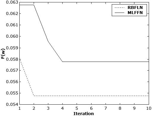

In step v, the goodness of fit of the models for the training data set was assessed (Table 7) by examining the mean absolute percentage error (MAPE), correlation coefficient ( $R$ ), squared correlation coefficient ( $Q^{2}$ ), root mean square error (RMSE) [32, 33], and the standard Akaike information criterion $\left(\textit{AIC}=T\log\left({\frac{\sum\left({y_{i}-\hat{y}_{i}}\right)^{2}}% {T}}\right)+2m\right)$ [34, 35, 36]. The Y-randomization test [37] was performed ten times for each of the models (Table 8), and the deviation between the mean squared correlation coefficient ( $Q_{r}^{2}$ ) of the randomized models and the squared correlation coefficient ( $Q^{2}$ ) of the non-randomized (original) model (Table 7) was reflected in the value of ${}^{C}R_{p}^{2}$ parameter [38] which should be more than 0.5 for a credible model. The calculated ${}^{C}R_{p}^{2}$ values (i.e., indicating that the presented models are robust) are given in Table 8. The external validations of the models were evaluated as centered on their $R(R_{\textit{ext}})$ , $Q^{2}(Q_{\textit{ext}}^{2})$ , $\textit{MAPE}(\textit{MAPE}_{\textit{ext}})$ and $\textit{RMSE}(\textit{RMSE}_{\textit{ext}})$ values for the data pairs in the testing data set (Table 9), and also the comparisons between the experimental and predicted solubility parameters using the network-based models are shown in Figs 6 and 7 along with the lines of perfect equality (i.e. the straight diagonal lines) and correlation coefficients. In addition, while the residuals of both models were plotted against the predicted values for the training and testing data sets in Figs 8 and 9, their applicability domains (AD) were verified by using the Williams plots (i.e., the plots of the cross-validated standardized residuals (SR) versus the leverage values [39]) shown in Figs 10 and 11.

Table 7

Internal validation results for the models

Model	$R$	$Q^{2}$	RMSE (J/cc) ${}^{0.5}$	MAPE (%)	AIC
RBFLNN-QSPR	0.939	0.883	1.147	4.650	40.98
MLFFNN-QSPR	0.937	0.876	1.178	4.730	111.11
GP-QSPR [4]	0.940	0.884	1.137	4.430	22.28
MLR-QSPR [4]	0.935	0.874	1.186	4.910	27.65

Table 8

The results of Y-randomization tests for the models

Randomization	Model
	RBFLN	MLFFN
	$Q^{2}$	$Q^{2}$
1	0.254	0.203
2	0.272	0.329
3	0.200	0.161
4	0.124	0.185
5	0.444	0.303
6	0.152	0.415
7	0.133	0.169
8	0.121	0.214
9	0.269	0.382
10	0.338	0.122
$Q_{r}^{2}$	0.230	0.248
${}^{C}R_{p}^{2}=\sqrt{Q^{2}}\sqrt{\left({Q^{2}-Q_{r}^{2}}\right)}$ [38]	0.758	0.741

Table 9

External validation results for the models

Model	$R_{\textit{ext}}$	$Q_{\textit{ext}}^{2}$	$\textit{RMSE}_{\textit{ext}}$ (J/cc) ${}^{0.5}$	$\textit{MAPE}_{\textit{ext}}$ (%)
RBFLNN-QSPR	0.980	0.947	0.385	1.680
MLFFNN-QSPR	0.980	0.928	0.447	1.920
GP-QSPR [4]	0.977	0.944	0.394	1.699
MLR-QSPR [4]	0.959	0.889	0.553	2.155

Figure 6.

Comparison between experimental and predicted solubility parameters by the RBFLN-QSPR model at the testing stage.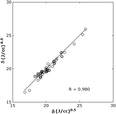

Figure 7.

Comparison between experimental and predicted solubility parameters by the MLFFN-QSPR model at the testing stage.

Figure 8.

The residuals versus predicted values for RBFLN-QSPR model.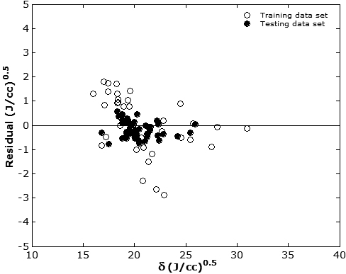

Figure 9.

The residuals versus predicted values for MLFFN-QSPR model.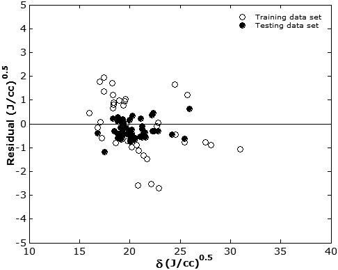

Figure 10.

William plot describing the applicability domain of RBFLN-QSPR model.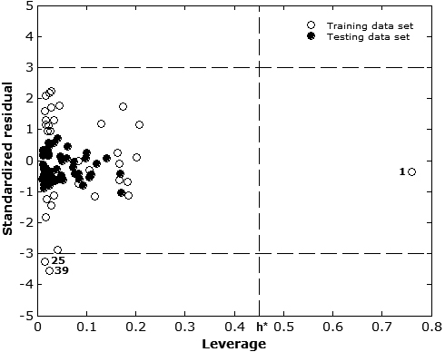

Figure 11.

William plot describing the applicability domain of MLFFN-QSPR model.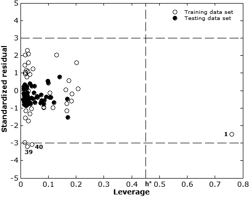

An analysis of the results is as follows:

In general, the good quality of the models can be indicated by small RMSE, MAPE and AIC values, $R$ , and $Q^{2}$ values close to one [26, 40]. As shown in Table 7, the models’ goodness of fit slightly differs from each other’s with respect to the internal validation measures $R$ , $Q^{2}$ , RMSE, MAPE except for AIC. The models with fewer parameters correspond to smaller AIC metrics, indicating a better balance/trade-off between complexity (i.e., the size of the vector of network parameters or the number of estimable model parameters) and accuracy (i.e., the goodness of fit) of the models. The AIC values revealed that the GP-QSPR produced the lowest AIC being the “best” model, while MLFFN-QSPR can be considered as the “worst” model with the greatest AIC (Table 7). On the other hand, Table 7, as well as, Table 9 also shows that not only the MLFFN-QSPR but also the RBFLN-QSPR had typically a tendency to require a relatively large amount of computational complexity in order to achieve similar or even better accuracy as with the GP-QSPR. As shown in Table 9, the RBFLN-QSPR model performed slightly better than the GP-QSPR model in terms of the $R_{\textit{ext}}$ , $\textit{RMSE}_{\textit{ext}}$ , $\textit{MAPE}_{\textit{ext}}$ and $Q_{\textit{ext}}^{2}$ values over the same testing data set. When also comparing the visual representations of correlations for the models (Figs 6 and 7) which measure the dispersion of the predictions around the perfect one, it is shown that the dispersion of results presented by the RBFLN-QSPR model in Fig. 6 is slightly less than that of the MLFNN-QSPR in Fig. 7. These results confirm that the GP [4] and RBFLN which combine the linear and nonlinear components in their buildings capture not only linear and but also nonlinear data structures in the relationship as opposed to the pure linear (MLR-QSPR) and non-linear (MLFFN-QSPR) models. That is why GP which is also a non-linear programming technique creates computer programs to solve a problem using Darwinian natural selection. It produces transparent solutions (i.e., algebraic expressions including linear and non-linear terms) similar to RBFLN but differs in the followings: GP does not require any formal structure selection as required in RBFLN (e.g., Eq. (1)), as well as, MLFFN (e.g., Eq. (2)) and MLR (e.g., $Y=WX$ with 1 $\times$ k dimensional weight matrix $W$ ) models. On the other hand, RBFLN includes a non-linear radial basis function (i.e., local-processing) model and additive linear (i.e., global-processing) model, while GP constructs a global function approximation, as is done by MLFFN and MLR models. This may explain that MLFFN, unlike RBFLN, shows a general high tendency to increase the number of hidden layer neurons in order to provide the best (lowest) values of the model selection metrics (Tables 5 and 6). On the other hand, compared to $\textit{AIC}_{ts}$ and $\textit{BIC}_{ts}$ , its lowest $\textit{AIC}_{tr}$ and $\textit{BIC}_{tr}$ scores indicate less number of hidden layer neurons, and this was the idea behind the using of $\overline{\textit{AIC}}$ and $\overline{\textit{BIC}}$ criteria to choose the best models. As a result, RBFLN-QSPR possessed faster speed of convergence and smaller steady error value than MLFFN-QSPR during the hybrid training process (Figs 4 and 5). This study also indicates that the presented hybrid optimization scheme may combine effectively a local (LM) and global (CS) search techniques for training of both neural networks. It can be noted here that CS presents an alternative initialization approach to the widely-used random initialization of points through the search space at the beginning of a local search process and thus confirms a good way of reducing the possibilities of falling into local minimum as well as computation time during the process of LM.

An analysis of Figs 8–11 show that i) the propagation of the residuals on both sides of zero line is random (meaning that the errors are normally distributed) and thus it can be concluded that no systematic error exists in the development of the RBFLN- and MLFFN-based QSPR models (Figs 8 and 9) ii) Both models perform well in terms of AD (Figs 10 and 11): The entire testing set compounds lie within the applicability domain (i.e., the squared area between $\pm$ 3 SR and the leverage threshold h ${}^{*}$ value) of the models. While the compound 1, poly (vinyl alcohol), in the training set lies outside the applicability domain and it can be considered as an influential compound, a few outliers were detected corresponding to compounds 39–25 (poly (vinyl methyl ketone); poly (vinyl ethyl ketone)) and 39–40 (poly (vinyl methyl ketone); poly (vinyl-1-amly methyl ether)) in the training data set for the RBFLN-(Fig. 10) and MLFFN-based (Fig. 11) models, respectively.

In this study, the implementations were performed using computer programs that were written in MATLAB run on an Intel Core i7 based PC.

4. Conclusions

This study investigates the development of RBFLN-based QSPR model to predict the solubility parameters of polymers. The results show that it outperforms MLFFN- as well as GP- and MLR-based QSPR models in terms of the external validation metrics and it includes the following advantages: i) RBFLN uses a global-and-local way of a general non-linear modelling to extract more information, while GP, MLR and MLFFN are globally tuned (i.e. linear or non-linear), ii) RBFLNN which produces much simpler structures than MLFFN can be implemented easily in practice. On the other hand, GP with the lowest AIC score can be preferred as a more practicable one to capture data structures with the least number of parameters. However, we noticed that GP differs from neural networks in that it constructs a mapping by optimizing its structure and parameters simultaneously and it has own limitations (e.g., difficulties in finding constants). This study also indicates that the hybridization of CS and LM algorithms effectively combines the local and global optimisation for the learning of neural networks

Footnotes

Conflict of interest

The authors declare that there is no conflict of interests.

References

Yousefinejad

and Hemmateenejad

, Chemometrics tools in QSAR/QSPR studies: A historical perspective, Chemometrics and Intelligent Laboratory Systems 149 (2015), 177–204.

Wang

and Gao

, Prediction of solubility parameters for polymers by a QSPR, QSAR Combinatorial Sci. 25(2) (2006), 156–161.

Goudarzi

Arab Chamjangali

and Amin

A.H.

, Calculation of Hildebrand solubility parameters of some polymers using QSPR methods based on LS-SVM technique and theoretical molecular descriptors, Chin J Polym Sci. 32(5) (2014), 587–594.

Koç

and Koç

M.L.

, A genetic programming-based QSPR model for predicting solubility parameters of polymers, Chemometrics and Intelligent Laboratory Systems 144 (2015), 122–127.

Looney

C.G.

, Radial basis functional link nets and fuzzy reasoning, Neurocomputing 48 (2002), 489–509.

Pao

Y.H.

Park

G.H.

and Sobajic

D.J.

, Learning and generalization characteristics of the random vector functional link net, Neurocomputing 6 (1994), 163–180.

Ahmadi

M.H.

Tatar

Nazari

M.A.

Ghasempour

Chamkha

A.J.

and Yan

W.M.

, Applicability of connectionist methods to predict thermal resistance of pulsating heat pipes with ethanol by using neural Networks, International Journal of Heat and Mass Transfer 126 (2018), 1079–1086.

Farzaneh-Gord

Mohseni-Gharyehsafa

Arabkoohsar

Ahmadi

M.H.

and Sheremet

M.A.

, Precise prediction of biogas thermodynamic properties by using ANN algorithm, Renewable Energy 147 (2020), 179–191.

Rabbi

K.M.

Sheikholeslami

Karim

Shafee

and Tlili

, Prediction of MHD flow and entropy generation by Artificial Neural Network in square cavity with heater-sink for nanomaterial, Physica A: Statistical Mechanics and its Applications 541 (2020), 123520.

10.

Ahmadi

M.H.

Mohseni-Gharyehsafa

Farzaneh-Gord

Jilte

R.D.

and Chau

K.W.

, Applicability of connectionist methods to predict dynamic viscosity of silver/water nanofluid by using ANN-MLP, MARS and MPR algorithms, Engineering Applications of Computational Fluid Mechanics 13(1) (2019), 220–228.

11.

Maddah

Aghayari

Ahmadi

M.H.

Rahimzadeh

and Ghasemi

, Prediction and modeling of MWCNT/Carbon (60/40)/SAE 10 W 40/SAE 85 W 90(50/50) nanofluid viscosity using artificial neural network (ANN) and self-organizing map (SOM), Journal of Thermal Analysis and Calorimetry 134 (2018), 2275–2286.

12.

Eswari

J.S.

Majdoubi

Naik

Gupta

Bit

Rahimi-Gorji

and Saleem

, Prediction of stenosis behaviour in artery by neural network and multiple linear regressions, Biomechanics and Modeling in Mechanobiology (2020), 1–15.

13.

Rahimi-Gorji

Ghajar

Kakaee

A.H.

and Ganji

D.D.

, Modeling of the air conditions effects on the power and fuel consumption of the SI engine using neural networks and regression, J Braz. Soc. Mech. Sci. Eng. 39 (2017), 375–384.

14.

Nawi

N.M.

Khan

and Rehman

M.Z.

, A new levenberg marquardt based back propagation algorithm trained with cuckoo search, Procedia Technology 11 (2013), 18–23.

15.

Toghyani

Ahmadi

M.H.

Kasaeian

and Mohammadi

A.H.

, Artificial neural network, ANN-PSO and ANN-ICA for modelling the Stirling engine, International Journal of Ambient Energy 37(5) (2016), 456–468.

16.

Asadi

Hadavandi

Mehmanpazir

and Nakhostin

M.M.

, Hybridization of evolutionary Levenberg-Marquardt neural networks and data pre-processing for stock market prediction, Knowledge-Based Systems 35 (2012), 245–258.

17.

Yang

X.S.

and Deb

, Multi objective cuckoo search for design optimization, Computers & Operations Research 40 (2013), 1616–1624.

18.

Yang

X.S.

and Deb

, Cuckoo search: Recent advances and applications, Neural Computing and Applications 24 (2014), 169–174.

19.

Kumar

and Rawat

T.K.

, Optimal fractional delay-IIR filter design using cuckoo search algorithm, ISA Transactions 59 (2015), 39–54.

20.

Ebenezer

N.G.R.

Ramabalan

and Navaneethasanthakumar

, Advanced design optimization on straight bevel gears pair based on nature inspired algorithms, SN Applied Sciences 1 (2019), 1155.

21.

Behnia

, Application of radial basis functional link networks to exploration for Proterozoic mineral deposits in Central Iran, Natural Resources Research 16(2) (2007), 147–155.

22.

Nykänen

, Radial basis functional link nets used as a prospectivity mapping tool for orogenic gold deposits within the central lapland greenstone belt, northern fennoscandian shield, Natural Resources Research 17(1) (2008), 29–48.

23.

Middleton

Närhi

and Sutinen

, Imaging spectroscopy in soil-water based site suitability assessment for artificial regeneration to Scots pine, ISPRS Journal of Photogrammetry and Remote Sensing 66 (2011), 287–297.

24.

Beucher

Österholm

Martinkauppi

Edén

and Fröjdö

, Artificial neural network for acid sulfate soil mapping: Application to the Sirppujoki River catchment area, south-western Finland, Journal of Geochemical Exploration 125 (2013), 46–55.

25.

Dash

P.K.

Nayak

Senapati

M.R.

and Lee

I.W.C.

, Mining for similarities in time series data using wavelet-based feature vectors and neural networks, Engineering Applications of Artificial Intelligence 20 (2007), 185–201.

26.

Koç

M.L.

Özdemir

Ü.

and İmren

, Prediction of the pH and the temperature-dependent swelling behavior of Ca2+-alginate hydrogels by artificial neural networks, Chemical Engineering Science 63 (2008), 2913–2919.

27.

and Wilamowski

B.M.

, Levenberg-marquardt training, Industrial Electronics Handbook: Intelligent Systems, 5(12) (2011), CRC Press.

28.

Ch’ng

S.I.

Seng

K.P.

and Ang

L.-M.

, Modular dynamic RBF neural network for face recognition, in: 2012 IEEE Conference on Open Systems, 2012, pp. 1–6.

29.

Xie

Hewlett

Rozycki

and Wilamowski

B.M.

, Fast and efficient second-order method for training radial basis function networks, IEEE Transactions on Neural Networks and Learning Systems 23(4) (2012), 609–619.

30.

Wilamowski

B.M.

and Yu

, Improved computation for levenberg-marquardt training, IEEE Transactions on Neural Networks 21(6) (2010), 930–937.

31.

and Zhang

G.P.

, An investigation of model selection criteria for neural network time series forecasting, European Journal of Operational Research 132 (2001), 666–680.

32.

Roy

and Kabir

, QSPR with extended topochemical atom (ETA) indices: Modeling of critical micelle concentration of non-ionic surfactants, Chemical Engineering Science 73 (2012), 86–98.

33.

Sheikholeslami

Gerdroodbary

M.B.

Moradi

Shafee

and Li

, Application of neural network for estimation of heat transfer treatment of Al2O3-H2O nanofluid through a channel, Comput. Methods Appl. Mech. and Engrg. 344 (2019), 1–12.

34.

Akaike

, A new look at the statistical identification model, IEEE Trans.Autom. Control 19 (1974), 716–723.

35.

Meango

T.J.

and Ouali

, Failure interaction models for multicomponent systems: A comparative study, SN Applied Sciences 1 (2019), 66.

36.

Badura

Batog

Drzeniecka-Osiadacz

and Modzel

, Regression methods in the calibration of low-cost sensors for ambient particulate matter measurements, SN Applied Sciences 1 (2019), 622.

37.

Wold

Eriksson

and Clementi

, Statistical validation of QSAR results, in: Chemometrics Methods in Molecular Design van de Waterbeemd

ed., Weinheim, VCH, 1995.

38.

Mitra

Saha

and Roy

, Exploring quantitative structure-activity relationship studies of antioxidant phenolic compounds obtained from traditional Chinese medicinal plants, Molecular Simulation 36(13) (2010), 1067–1079.

39.

Eriksson

Johansson

Müller

and Wold

, On the selection of the training set in environmental QSAR analysis when compounds are clustered, J Chemometrics 14 (2000), 599–616.

40.

Koç

M.L.

Balas

C.E.

and Koç

, Stability assessment of rubble-mound breakwaters using genetic programming, Ocean Engineering 111 (2016), 8–12.

QSPR prediction of polymers’ solubility parameters by radial basis functional link net

Abstract

Keywords

1. Introduction

2. Theory and calculation

Table 1 Ranges of inputs and output ( δ ) variables in the training data set [4]

Footnotes

Conflict of interest

References

Table 1
Ranges of inputs and output ( $\delta$ ) variables in the training data set [4]