Hyperspectral remote sensing image dimensionality reduction method based on adaptive filtering

Abstract

With the rapid development of hyperspectral image technology, remote sensing technology has ushered in an innovation in theory and application, and hyperspectral remote sensing images have come into being. However, due to its high data dimensionality, it is difficult for statistical classifiers to work on it, making the technology face development difficulties. Therefore, how to effectively reduce the dimensionality of hyperspectral remote sensing images has gradually become a research hotspot in this field. The study clusters bands by K-means algorithm, and then combines the least mean square algorithm in adaptive filtering and recursive least squares method, and uses this as the basis for band selection. Finally, the dimension reduction effect is verified. The experimental results show that the improved band selection method achieves an overall accuracy of over 80% and 90% in the hyperspectral datasets of Pavia University and Idian Pine respectively, with the Kappa coefficient reaching 0.9. In the overall dimensionality reduction classification of the Indianan data, the accuracy also reaches 90% and can be maintained consistently, indicating that the method has high accuracy and can effectively reduce the dimensionality of hyperspectral remote sensing images.

Keywords

Adaptive filtering minimum mean algorithm K-means hyperspectral remote sensing image dimensionality reduction

1. Introduction

Remote sensing is capable of dynamic observation of a wide range of environments, regardless of weather, human factors and geographical location, and is widely used in ecological research, environmental detection and mapping [1]. The processing of remote sensing images covers image acquisition, denoising, compression and feature classification, and as an important part of remote sensing image processing, feature classification is of great importance in both civil and military fields. As the temporal, spatial and spectral resolution of remote sensing images continues to increase, dynamic observation data becomes more complex. At the same time, hyperspectral imaging technology has led to a significant increase in the volume of data, both of which have led to frequent “dimensional catastrophe” problems [2]. For example, as the spectral band increases with a certain training sample, classifiers such as support vector machines experience a decrease in accuracy as the number of feature dimensions increases [3]. In addition, hyperspectral remote sensing images are characterized by rich implied features, narrow and many band widths, and large data redundancy, which cause great difficulties for data processing accuracy. At present, for hyperspectral remote sensing image dimensionality reduction is mainly achieved by band selection methods. And adaptive filtering as an information processing method has a broad development prospect in hyperspectral remote sensing images. In contrast, at present, the dimensionality reduction method of hyperspectral remote sensing images still does not achieve practical results, and the accuracy obtained by wavelet selection classification is still high [4]. Therefore, the study was conducted by performing band selection based on adaptive filtering and clustering using the K-means algorithm with a view to improving the classification accuracy and the efficiency of hyperspectral remote sensing image dimensionality reduction.

2. Related work

Hyperspectral remote sensing has high feature dimensionality and high spectral resolution, but problems such as data redundancy have been limiting its development and application. Wang and Liu [5] developed a pre-dimensionalisation algorithm combining a dictionary of thin eigenmodes and a weighted low-rank representation to improve the performance of linear discriminant analysis by seeking a low-rank subspace, Le et al. [6] proposed a new neural network method to classify hyperspectral CO ${}_{2}$ remote sensing images, and evaluated the classification accuracy using local standard deviation and local mean of the spectral images, and the results showed that it improved the classification efficiency and accuracy of remote sensing data and accuracy. Zhao et al. [7] proposed a non-linear feature extraction method for hyperspectral images to address the problem of information redundancy caused by increasing spectral dimensionality, and effectively estimated the noisy part of the image by exploring the characteristics of the use of image segmentation, and the results showed that it improved the classification performance. Akyürek and Koer [8]proposed a semi-supervised feature extraction method for semi-supervised fuzzy neighbourhood preservation analysis in order to improve the inefficiency of image feature extraction, and improved the classification accuracy by using a limited number of labelled data, and the experimental results demonstrated the high operational effectiveness of the algorithm. Hong et al. [9] optimized the high-level data analysis the preprocessing step, a semi-supervised method of iterative multi-task regression was used to bridge the learned subspaces by two regression tasks, given the pseudo-tags and tokens initialised by the classifier, and the results showed its high performance in terms of classification and recognition accuracy. Zeng et al. [10] tackled the problem of hyperspectral high dimensionality by using a weighted spatial spectrum and global-local discriminant analysis algorithm to extract image features and add samples with high classification confidence to the training set through an incremental learning strategy, which was shown to reduce the misclassification probability.

Duan et al. [11] artificially extracted the structural features of hyperspectral images and proposed a new multiscale all-variable method, which first reduced the spectral dimension by averaging method, and obtained accurate data for classification before using kernel principal component analysis, and experimental results on three hyperspectral datasets showed that the method had strong robustness. Sun et al. [12] artificially reduced the hyperspectral spectral images with mixing noise, proposed a low-rank representation method, which develops a spectral difference space by differencing images along the kernel parametrization of spectral for, and conducted experiments on simulated and real datasets, and the results showed that the method improved the quality of visual evaluation. Zhao and Lu [13] proposed a multimodal image fusion denoising variational model, which uses a multi-scale alternating sequence filter to extract useful features of the image and guides the fusion of the main features of the input through the weight map of the recursive filter, and the results show that it improves the quality of fusion. Xie et al. [14] proposed an unsupervised clustering method based on pixel spacing and spectral space pixel density in order to optimize the ensemble differences of remote sensing images. supervised clustering method and measured the distance by an adaptive generational width probability density function, and validated the good classification effect of the method by comparing it with a reference dataset. Zhang et al. [15] developed a joint spatial-spectral classification method that maintains edge and localization for the problem of strong spatial neighbourhood correlation in HSI classification, and used guided filtering to extract the spatial features of each band separately, and then classify them using a random forest classifier, which was shown to improve the classification effect. Han et al. [16] proposed a time-weighted collaborative filtering algorithm to improve small-batch K-means clustering for sparse scoring matrix to cluster and derive user scores with high recall and scoring prediction accuracy. Li et al. [17] proposed an improved affine projection subband adaptive filter for dealing with noisy environments with high backgrounds, which was obtained by minimizing the difference between the updated tapped weighting vector and the past weighting vector, and the results showed that the method achieves lower steady-state misalignment.

In summary, most researchers have achieved better classification results by dimensionality reduction processing of hyperspectral remote sensing images from the aspect of classification accuracy, but there is relatively little research on the application of adaptive filters in image dimensionality reduction and a lack of research on relevant improvement algorithms for adaptive filters. Therefore, the study carries out band selection by introducing K-means algorithm and adaptive filtering to improve classification accuracy and promote the speed and efficiency of processing hyperspectral remote sensing images.

3. Hyperspectral remote sensing image dimensionality reduction based on adaptive filtering

3.1 Waveband selection based on adaptive filtering

Adaptive filtering estimates the error by the expected response and the input vector, thereby updating the filter coefficients, and its ability to capture local statistical features of unknown systems or non-stationary environments without the need for a priori knowledge based on data statistics can achieve better filtering results than fixed filters [18, 19]. The Least Mean Square (LMS) algorithm, as the most widely used algorithm in adaptive filtering, has the advantages of robustness and structural simplicity. The LMS algorithm is a gradient-fastest descent algorithm, which is updated along the negative direction of the gradient valuation as the filter weight coefficients are iterated. The vector signal flow chart of the LMS algorithm is shown in Fig. 1.

Figure 1.

Vector signal flow chart of LMS algorithm.

The LMS algorithm first selects a suitable step factor and number of taps for the filter, and then performs an initialization with an equation initial weight value of 0 [20]. The signal error is then calculated from the desired signal, input signal and vector valuation, and an update of the weight factor estimate is performed, and finally 1 is added to the existing time index and the process is repeated until the steady state position. The gradient equation of the LMS algorithm is shown in Eq. (1).

$\displaystyle\hat{\nabla}_{n}=\frac{\partial[e^{2}(n)]}{\partial W}=2e(n)\frac% {\partial e(n)}{\partial W}=-2X(n)e(n)$ (1)

In Eq. (1), $X(n)$ represents input sampling, $e^{2}(n)$ represents the squared error and $W$ is the vector of coefficients. The gradient expression enables the vector iteration equation of the LMS algorithm to be obtained, as shown in Eq. (2).

$\displaystyle W(n+1)=W(n)-\mu\hat{\nabla}_{n}=W(n)+2X(n)\mu e(n)$ (2)

In Eq. (2), $\mu$ represents the iteration step size and $\mu>0$ , by choosing the appropriate value of $\mu$ can achieve a better convergence performance of the algorithm. In the fastest descent method, the mutual and autocorrelation matrices must be determined in order to accurately measure the gradient vector, but this is difficult to achieve in an unknown environment. This problem is therefore addressed by combining another algorithm from adaptive filtering, recursive least squares (Least Square, LS). Recursive least squares have the advantages of better tracking ability and speed, and has been successfully applied in inter-spectral linear prediction. Its cost function is shown in Eq. (3).

$\displaystyle J_{n}(w)=\delta\lambda^{n}\left\|{w(n)}\right\|^{2}+\sum\limits_% {i=1}^{n}\lambda^{n-i}\left|{e(i)}\right|^{2}$ (3)

In Eq. (3), $\lambda$ represents the forgetting factor, $\delta$ represents the regularisation parameter, $\delta\lambda^{n}\left\|{w(n)}\right\|^{2}$ represents the regularisation term and $e(i)$ represents the estimation error. The forgetting factor is used to ‘forget’ the old data and can only track the statistics of the observed data when it is not stable, while the regularisation term is used to solve the stable problem. It is differentiated by the cost function so that the result is equal to zero, and the inverse gravity of the matrix is given by the equation shown in Eq. (4).

$\displaystyle\Phi^{-1}(n)=\lambda^{-1}\Phi^{-1}(n-1)-\Phi^{-1}(n-1)\lambda^{-1% }k(n)u^{T}$ (4)

In Eq. (4), $\Phi$ represents the inverse correlation matrix and $k(n)$ represents the gain vector. The resulting recursive estimate of the filter coefficients is shown in Eq. (5).

$\displaystyle\hat{w}(n)=\hat{w}(n-1)-e^{\ast}(n)k(n)$ (5)

In Eq. (5), $e^{\ast}$ represents the a priori estimation error. The combination of the least mean square algorithm and recursive least squares can achieve good results in terms of block convergence and low complexity. Based on the adaptive filtering combined with the two algorithms, the band selection algorithm combining Principal Component Analysis (PCA) and Mutual Information was selected for hyperspectral remote sensing images. The reference band source is the data obtained from the principal component analysis, the similarity measure of the bands is the Mutual Information, and finally the bands are selected by KL scatter (Kullback-Leibler divergence). The principal component analysis method is based on a linear transformation that makes its components uncorrelated and will reduce the amount of information as the principal component number increases [21]. The covariance and variance of all vectors are shown in Eq. (6).

$\displaystyle\left\{{\begin{array}[]{ll}\textit{Var}=a_{i}^{T}\sum a_{i},&i=1,% 2,\cdots,p\\ \textit{Cov}(z_{i},z_{j})=a_{i}^{T}\sum a_{j},&i,j=1,2,\cdots,p\\ \end{array}}\right.$ (6)

In Eq. (6), $\textit{Var}(z_{i})$ represents the variance of the vector $z_{i}$ and $\textit{Cov}(z_{i},z_{j})$ represents the covariance of $z_{j}$ and $z_{i}$ such that the transformation matrix satisfies: $a_{1}^{T}a_{1}=1$ , then $z_{1}$ is the first principal component. The conditional extremum problem for the first principal component in the principal hierarchy analysis requires certain conditions to be considered, as shown in Eq. (7).

$\displaystyle\left\{{\begin{array}[]{l}\frac{\partial\varphi}{\partial\lambda}% =a_{1}^{T}a_{1}-1=0\\ \\ \frac{\partial\varphi}{\partial a_{1}}=2\left(\sum-\lambda I\right)a_{1}=0\\ \end{array}}\right.$ (7)

In Eq. (7), is the $\lambda$ parameter and $\varphi$ represents the Lagrangian function. It can be seen that solving Eq. (7) means solving for the eigenvectors and eigenvalues of $\sum$ , and then using the mutual information to obtain the similarity measure of the bands. The mutual information determines how similar the product of the marginal probability distribution and the joint probability distribution is. The mutual information is positively correlated with the correlation of the two vectors, i.e. the greater the correlation, the greater the mutual information of the two variables and the more similar they are [22]. The mutual information of two discrete random vectors is shown in Eq. (8).

$\displaystyle I(X,Y)=\sum\limits_{x\in X}{\sum\limits_{y\in Y}{p(x,y)}}\log% \frac{p(x,y)}{p(y)p(x)}$ (8)

In Eq. (8), $X$ and $Y$ represent the discrete vectors, $I$ represents the mutual information, $p(x)$ and $p(y)$ represent the edge probabilities of the two discrete vectors, and $p(x,y)$ is the joint probability distribution of these two vectors. Therefore, the relationship between information entropy and mutual information is obtained by the equation shown in Eq. (9).

$\displaystyle I(X,Y)\left\{{\begin{array}[]{l}=H(X)-H(X|Y)=H(Y)-H(Y|X)\\ =H(Y)+H(Y)-H(X,Y)\\ \end{array}}\right.$ (9)

In Eq. (9), $H(X)$ and $H(Y)$ represent the entropy of $X$ and $Y$ respectively, $H(X|Y)$ and $H(Y|X)$ both represent the conditional entropy, and $H(X,Y)$ represents the joint entropy of the two. The relationship between information entropy and mutual information is shown in Fig. 2.

Figure 2.

Graph of information entropy and mutual information.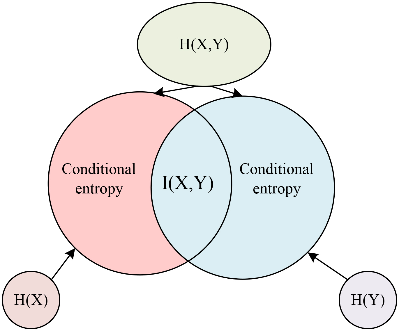

The degree of similarity between the two variables is then measured by the KL scatter, which is the directional scatter of the two distributions. KL scatter describes the amount of additional information about the variable that differs from it through a random variable, is a characterisation of the differences between the two variables, and is able to describe the correlation between the bands and thus remove the band that is similar to the current band without causing a large loss after removal [23]. Therefore, the whole band selection method is to first transform the obtained dataset using principal component analysis and then select the current optimal band using mutual information. The reference band is then updated by KL coefficients to continuously obtain the optimal band, and the optimal band set after repeated iterations is the target low-dimensional data.

3.2 Wave clustering based on K-means algorithm

Before band selection, bands of hyperspectral images need to be clustered, and K-means algorithm is selected for corresponding processing. The K-means algorithm is an iterative clustering algorithm with the advantages of simplicity, efficiency and interpretability, and is widely used in pattern recognition and data clustering [24]. Firstly, a certain amount of sample data needs to be selected to form the initial clustering centres, and then the similarity measure function is used to obtain the distance between each clustering centre and other sample data in the given data set. The sample data is then assigned, and the assignment process involves selecting the nearest cluster class as the target by comparing its distances to all cluster centres. After all the sample data has been assigned to the target cluster class, the mean value of each sample data in the cluster class is calculated to determine if there is a need to move the cluster centre. If there is a need to move, the clusters are re-classified using an iterative method until there is no change in all the sample data, as shown in Fig. 3.

Figure 3.

Schematic diagram of K-means.

The K-means algorithm to divide data samples needs to measure the similarity between samples, which is mainly expressed through the Euclidean distance, as shown in Eq. (10).

$\displaystyle d(x_{i},x_{j})=\sqrt{\sum\limits_{k-1}^{n}{(x_{ik}-x_{jk})^{2}}}$ (10)

In Eq. (10), the data samples are denoted by $x_{j}$ and $x_{i}$ , while $x_{ik}$ and $x_{jk}$ denote the data samples located in the $k$ cluster class. The mean squared deviation is the objective criterion function in the K-means algorithm, as shown in Eq. (11).

$\displaystyle E=\sum\limits_{j=1}^{c}\sum\limits_{k=1}^{n_{j}}{\left\|{x_{k}-m% _{j}}\right\|}^{2}$ (11)

In Eq. (11), $x_{k}$ is the data element, $m$ is the cluster centre and $E$ is the sum of the mean squared deviations obtained from the data elements. The independence between clusters and the compactness within clusters are determined by whether the clusters can find the optimal division, and the criterion is the sum of squared errors, as shown in Eq. (12).

$\displaystyle\left\{{\begin{array}[]{l}c_{i}=\frac{1}{N_{i}}\sum\limits_{% \begin{subarray}{c}j=1\\ x_{j}\in C_{i}\end{subarray}}^{n}{x_{j}}\\ J=\sum\limits_{i=1}^{k}\sum\limits_{\begin{subarray}{c}j=1\\ x_{j}\in C_{i}\end{subarray}}^{n}{\textit{dis}(x_{j},c_{i})}^{2}\\ \end{array}}\right.$ (12)

In Eq. (12), $x_{j}$ represents the data sample, located in the class $C_{i}$ , $N_{i}$ represents the number of data objects, and $c_{i}$ is the mean value of the data objects. The K-means algorithm is introduced to hyperspectral images, and the initial clustering centres are then equal-step wavebands. The sample data are also divided according to the Euclidean distance so that the more similar sample data are located in the same cluster class, and the sample data between dissimilar cluster classes are less similar. The iterative clustering centre is the mean of the bands, and the representative band is the band closest to the cluster centre, as shown in Fig. 4.

Figure 4.

K-means algorithm band clustering flow chart.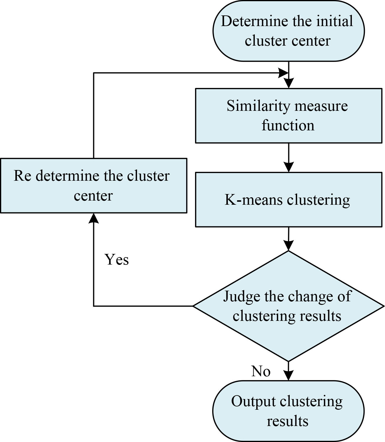

The K-means algorithm clusters the bands of the hyperspectral images and the resulting set of bands is shown in Eq. (13).

$\displaystyle M=\{{m_{i}|{m_{i}=(m_{i1},m_{i1},m_{i1},\cdots,m_{in}),i=1,2,3% \cdots,l}}\}$ (13)

In Eq. (13), $l$ is the total number of bands, $M$ is the set of bands, and $m_{i}$ represents the $n$ dimensional vector of bands with the sequence $i$ , which also has $n$ different attributes. Thus, the initial clustering of the central bands can be shown by Eq. (14).

$\displaystyle W=\{{w_{i}|{w_{i}=(w_{i1},w_{i2},\cdots,w_{in}),i=1,2,\cdots,k}}\}$ (14)

In Eq. (14), $k$ is the number of clusters, and $w_{i}$ represents the $n$ dimensional vector of the clustering center band sequence as $i$ . The equation of the Euclidean distance between the clustering central band and any band is then derived from the equation of the clustering central band in the iterative process, as shown in Eq. (15).

$\displaystyle w_{j}=\frac{\sum\limits_{g=1}^{l_{j}}{m_{j}}}{n_{j}},j=1,2,% \cdots,k;g=1,2,\cdots,n;j=1,2,\cdots,k$ (15)

In Eq. (15), $n_{j}$ denotes the total number of bands for which the clustering sequence is $j$ .

Figure 5.

Overall accuracy results of four algorithms in Idian pine data.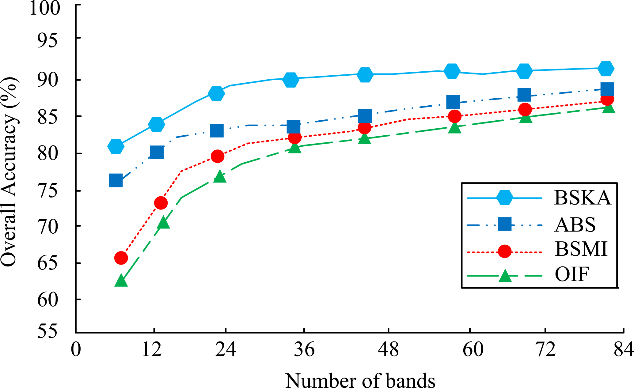

4. Dimension reduction effect of hyperspectral remote sensing image based on band selection

To validate the effectiveness of the proposed band selection method, comparison tests were conducted on two hyperspectral datasets, Idian Pine and Pavia University, respectively, and the reduced dimensionality data were validated by maximum likelihood classification. For the post-classification evaluation, two metrics, Kappa coefficient and Overall Accuracy (OA), were selected. The proposed Band Selection method combining K-means and Adaptive filtering (BSKA) and Adaptive Band Selection (ABS), based on Band Selection algorithm based on Maximum Information (BSMI) and Optimum Index Factor (OIF) were compared. The overall accuracy results of the four algorithms in the Idian Pine data are shown in Fig. 5.

As can be seen from Fig. 5, the overall accuracy of all four algorithms for classification increases with the number of bands selected. The overall accuracy of the BSKA algorithm exceeds 80% at the lowest level, and increases steadily as the number of bands increases, reaching a maximum of over 90%, which is a good classification result. The overall accuracy of the ABS algorithm was between 75% and 80% at the lowest, and increased slightly with the number of bands, but the highest accuracy did not exceed 90%, which was still different from the BSKA algorithm. The BSMI and OIF algorithms are both in the range of 55%–70% at the lowest and 85% at the highest, with average classification results, far below the classification accuracy of the BSKA algorithm. The results of Kappa coefficients for all four in the Idian Pine data are shown in Fig. 6.

Figure 6.

Kappa coefficient results of the four in Idian pine data.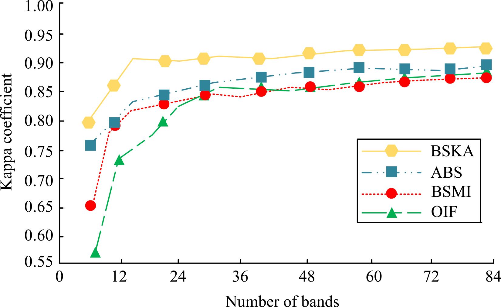

As can be seen from Fig. 6, the Kappa coefficient increases as the number of bands increases. the Kappa coefficient of the BSKA algorithm reaches around 0.87 when the number of bands increases to 12, while the ABS, BSMI and OIF algorithms are 0.84, 0.65 and 0.56, respectively, which differ significantly from the BSKA algorithm. When the number of bands increases to around 80, the Kappa coefficients for all four algorithms reach a maximum, with BSKA being the largest at 0.9. Combining this with Fig. 5 shows that the Kappa coefficients and OA follow roughly the same trend. When the number of bands exceeds 24, the Kappa coefficients and OA of all four algorithms grow slowly, indicating that all four are close to the optimal bands. And from the magnitude of the Kappa coefficient and OA values obtained by all four, the BSKA algorithm outperformed the other three algorithms and showed better classification results. The four algorithms were then placed in the dataset Pavia University, which has a smaller number of bands compared to Idian Pine and has a higher resolution of hole home. Therefore, the number of bands was set to 3:2:33 and the experimentally selected data was classified by the Bayesian classification algorithm and the overall accuracy results obtained are shown in Fig. 7.

Figure 7.

Overall accuracy results of four algorithms in Pavia University.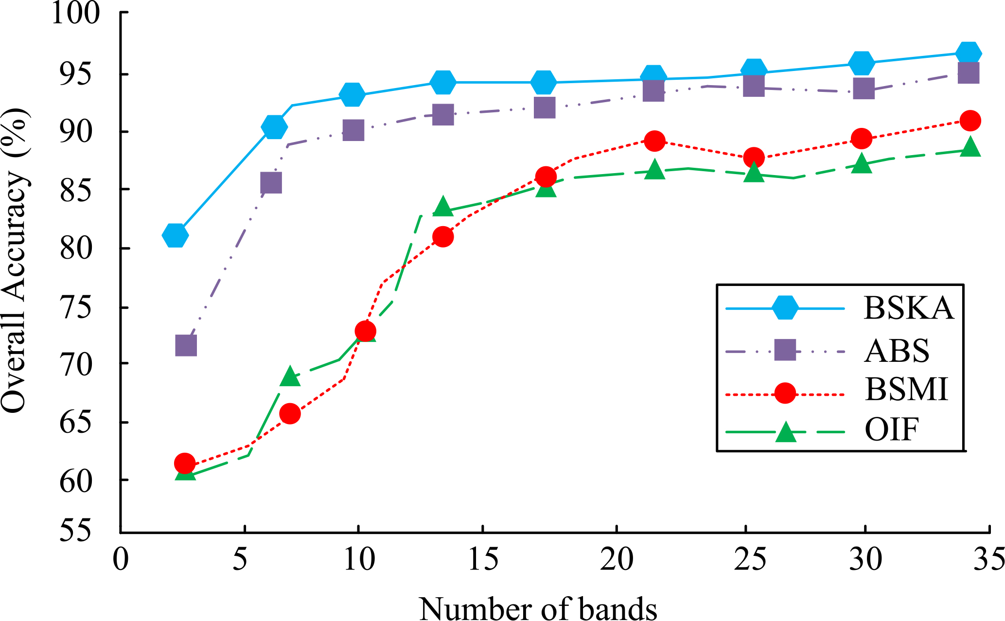

As can be seen from Fig. 7, with an initial band number of 3, the overall accuracy of the BSKA algorithm can reach 80% and that of the ABS algorithm is 74%, while both BSMI and OIF are only 60%. The overall accuracy of BSKA is improved by 6% compared to ABS and 20% compared to BSMI and OIF, and the classification effect is improved more obviously. When the number of bands is 7, the overall accuracy of BSKA is 88% and ABS is 80%, while the other two algorithms are between 60% and 70%, with BSKA still leading. At a band count of 33, BSKA achieves the highest overall accuracy of 96%, with the other three algorithms all around 90%, still lower than the improved algorithm. The Kappa coefficients in the dataset Pavia University are shown in Fig. 8.

Figure 8.

Kappa coefficient in data set Pavia University.

As can be seen from Fig. 8, when the number of bands is 3, the Kappa coefficient of the BSMI and OIF algorithms is only 0.2, with a poor classification effect, the ABS algorithm is between 0.4 and 0.5, with an average classification effect, while the BSKA algorithm reaches 0.6, with a better classification effect than the other three algorithms. Combined with the overall accuracy of the four in Fig. 7, it can be seen that the Kappa coefficient and overall accuracy of the ABS algorithm are closer to those of the BSKA algorithm, indicating that the similarity between the two obtained bands is greater at this point, but the BSKA algorithm still has better results than the ABS algorithm. When the number of bands exceeds 25, the overall accuracy of BSMI reaches 85% and above, and the Kappa coefficient at this point is close to and exceeds 0.7, indicating that the effect of BSMI only appears better when the number of bands selected is large enough. The Kappa coefficient of OIF only exceeds 0.7 when the number of bands exceeds 30, which is slightly less effective than BSMI and far less effective than ABS and BSKA. Therefore, the BSKA algorithm outperforms the other three algorithms, regardless of the number of bands selected. To further validate the performance of the proposed BSKA algorithm, it was applied to real image downscaling, i.e. the overall downscaling classification of the Indianan data. The real features in the full image were obtained from the real reports of the features as shown in Table 1.

Table 1

Real surface features in the whole map

Category	Corresponding figure	Number of samples
A1	Corn	241
A2	Stone-steel towers	97
A3	Woods	1347
A4	Wheat	208
A5	Oats	26
A6	Soybeans-min	2455
A7	Hay-windrowed	486
A8	Soybeans-clean	602
A9	Grass/tress	765
A10	Soybeans-notill	991
A11	Alfalfa	48
A12	Corn-notill	1496
A13	Grass/pasture	489
A14	Corn-min	862
A15	Bldg-Grass-Tree-Drivers	388
A16	Grass/pasture-mowed	30

From Table 1, it can be seen that there are 16 classes of features in the full map, among which Soybeans-min has the largest number of samples, 2455, and Grass/pasture-mowed and Oats have the smallest number of samples, 30 and 26 respectively. Full map classification experiments were then conducted, and the classification results of the four obtained algorithms with different dimensionality reduction are shown in Fig. 9.

Figure 9.

Classification results under different dimensionality reduction dimensions.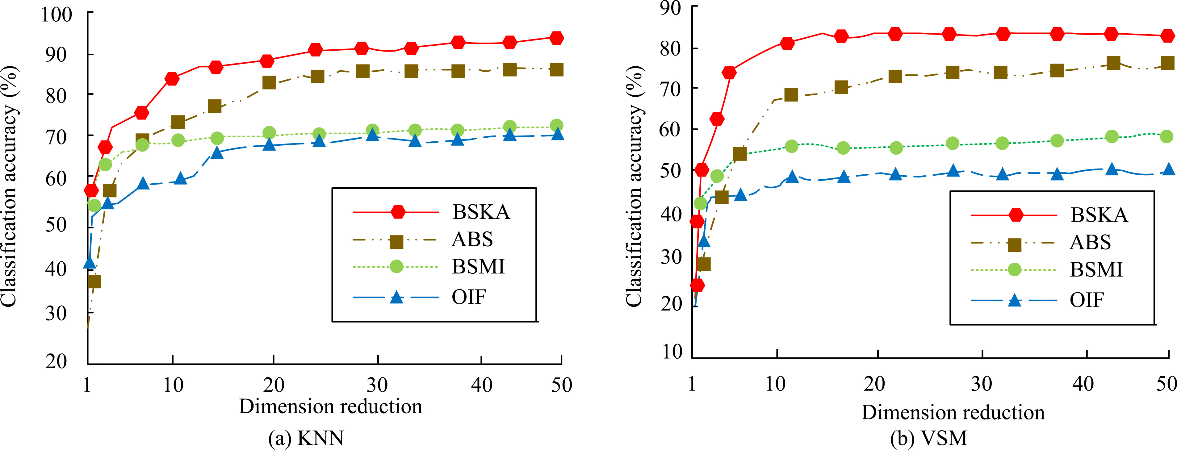

In Fig. 9, subplot (a) shows the classification results obtained by the four algorithms under the K-nearsestneighbor (KNN) method, and subplot (b) shows the results obtained by VSM. The classification accuracy of the BSMI and OIF algorithms increased from about 20% to a peak around 60%, and the accuracy was relatively low. The accuracy of the BSKA algorithm stabilises at 90% after increasing the dimensionality to 20, which is better. As can be seen from Fig. 9b, under VSM, the accuracy of the OIF and BSMI algorithms stabilised at 40%–50% and 50%–55% respectively after the dimensionality increased to 15, while the BSKI algorithm stabilised at 80% and above, which is still about 10% higher than the ABS algorithm and has a higher accuracy and classification effect. Therefore, both under KNN and VSM, the proposed BSKA algorithm can obtain high accuracy and outperform the other three algorithms.

5. Conclusion

Hyperspectral remote sensing image technology has been successfully applied in many fields such as military reconnaissance and modern agriculture, but the huge amount of data makes its transmission and storage a new challenge. The research is based on adaptive filtering, which combines principal component score and mutual information for band selection to improve classification accuracy and achieve image dimensionality reduction.

The experimental results show that the OA values of the ABS algorithm range from 75% to 88% in the Idian Pine data, and the OA values of the BSKA algorithm classification are above 80%, up to over 90%, and remain stable. The Kappa coefficients of the BSMI, ABS and OIF algorithms were 0.65, 0.84 and 0.56 respectively for a band count of 12, while the BSKA algorithm reached 0.87 and reached a maximum of 0.9 for a band count of 80. Within Pavia University, the overall accuracy of BSKA reached a maximum of 96%, while the OIF, BSMI and ABS algorithms were all around 90%.

In terms of Kappa coefficient, the BSKA algorithm is the highest at 0.9, which is better than the other three algorithms. In experiments on feature classification, the classification accuracy of the BSKA algorithm under KNN is stable at around 90% with increasing dimensionality, and the BSKI algorithm under VSM is stable at more than 80%, which is higher than the other three algorithms, with higher accuracy and better classification, and can perform high-performance dimensionality reduction on hyperspectral images. However, the algorithm proposed in the study has the problem of long time spent in iterative waveband selection, so further improvement is needed to improve the algorithm operation efficiency.

Footnotes

Funding

The research is supported by: Key research project of natural science of Anhui Provincial Department of Education, Research on substation temperature detection based on Intelligent Data Fusion, (No. KJ2020A0814); School level key scientific research fund project of Anhui Wenda University of Information Engineering, Research on fog penetration algorithm of video device in bad weather, (No. XZR2021A09).

References

Duan

Huang

Tang

. Semisupervised manifold joint hypergraphs for dimensionality reduction of hyperspectral image. IEEE Geosci Remote Sens Lett. 2020; 18(10): 1-5.

Wang

Yuan

. GETNET: A general end-to-end 2-D CNN framework for hyperspectral image change detection. IEEE Trans Geosci Remote Sens. 2018; 57(1): 3-13.

Wang

Zheng

Xiong

. Hyperspectral image dimensionality reduction via graph embedding in core tensor space. IEEE Geosci Remote Sens Lett. 2020; 18(3): 509-513.

Jain

Tyagi

. An adaptive edge-preserving image denoising technique using patch-based weighted-SVD filtering in wavelet domain. Multimedia Tools Appl. 2017; 76(2): 1659-1679.

Wang

Liu

. Weighted low-rank representation-based dimension reduction for hyperspectral image classification. IEEE Geosci Remote Sens Lett. 2017; 14(11): 1938-1942.

Zhang

Wang

. Classification method of CO2 hyperspectral remote sensing data based on neural network. Comput Commun. 2020; 156: 124-130.

Zhao

Gao

Liao

Zhang

. A new kernel method for hyperspectral image feature extraction. Geo-Spatial Inf Sci. 2017; 20(4): 309-318.

Akyürek

Koer

. Semi-supervised fuzzy neighborhood preserving analysis for feature extraction in hyperspectral remote sensing images. Neural Comput Appl. 2019; 31(8): 3385-3415.

Hong

Yokoya

Chanussot

Zhu

. Learning to propagate labels on graphs: an iterative multitask regression framework for semi-supervised hyperspectral dimensionality reduction. ISPRS J Photogrammetry Remote Sens. 2019; 158: 35-49.

10.

Zeng

Wang

Gao

Kang

Feng

. Hyperspectral image classification with global-local discriminant analysis and spatial-spectral context. IEEE J Sel Top Appl Earth Obs Remote Sens. 2019; 11(12): 5005-5018.

11.

Duan

Kang

Ghamisi

. Noise-robust hyperspectral image classification via multi-scale total variation. IEEE J Sel Top Appl Earth Obs Remote Sens. 2019; 12(6): 1948-1962.

12.

Sun

Jeon

Zheng

. Hyperspectral image restoration using low-rank representation on spectral difference image. IEEE Geosci Remote Sens Lett. 2017; 14(7): 1151-1155.

13.

Zhao

. Medical Image fusion and denoising with alternating sequential filter and adaptive fractional order total variation. IEEE Trans Instrum Measure. 2017; 66(9): 2283-2294.

14.

Xie

Zhao

Huang

Han

Liu

, et al. Unsupervised hyperspectral remote sensing image clustering based on adaptive density. IEEE Geoence Remote Sens Lett. 2018; 15(4): 632-636.

15.

Zhang

Liu

. Spatial-spectral joint classification of hyperspectral image with Locality and edge preserving. IEEE J Sel Top Appl Earth Obs Remote Sens. 2020; 13: 2240-2250.

16.

Han

Wang

. Time-weighted collaborative filtering algorithm based on improved mini batch K-Means clustering. Adv Sci Technol. 2021; 105: 309-317.

17.

Zheng

Wang

Zhou

. Ensemble EMD-based spectral-spatial feature extraction for hyperspectral image classification. IEEE J Sel Top Appl Earth Obs Remote Sens. 2020; 13: 5134-5148.

18.

Crawford

Zhu

Liu

. Centroid and covariance alignment-based domain adaptation for unsupervised classification of remote sensing images. IEEE Trans Geosci Remote Sens. 2018; 57(4): 2305-2323.

19.

Feng

Wang

. Hyperspectral image dimension reduction using weight modified tensor-patch-based methods. IEEE J Sel Top Appl Earth Obs Remote Sens. 2020; 13: 11-16.

20.

Liao

Wang

Hao

. Hyperspectral image classification based on adaptive optimisation of morphological profile and spatial correlation information. Int J Remote Sens. 2018; 39(23): 9159-9180.

21.

Feng

Shang

Sui

Jiao

, et al. Attention multibranch convolutional neural network for hyperspectral image classification based on adaptive region search. IEEE Trans Geosci Remote Sens. 2020; 59(6): 5054-5070.

22.

Baisantry

Sao

Shukla

. Band selection using combined divergence-correlation index and sparse loadings representation for hyperspectral image classification. IEEE J Sel Top Appl Earth Obs Remote Sens. 2020; 13: 5011-5026.

23.

Mei

Hou

Chen

Chau

. Simultaneous spatial and spectral low-rank representation of hyperspectral images for classification. IEEE Trans Geosci Remote Sens. 2018; 56(5): 1-15.

24.

Ali

Wasid

. Multi-criteria clustering-based recommendation using Mahalanobis distance. Int J Reasoning-Based Intell Syst. 2020; 12(2): 96-108.