LSTM network optimization and task network construction based on heuristic algorithm

Abstract

This work aims to advance the security management of complex networks to better align with evolving societal needs. The work employs the Ant Colony Optimization algorithm in conjunction with Long Short-Term Memory neural networks to reconstruct and optimize task networks derived from time series data. Additionally, a trend-based noise smoothing scheme is introduced to mitigate data noise effectively. The approach entails a thorough analysis of historical data, followed by applying trend-based noise smoothing, rendering the processed data more scientifically robust. Subsequently, the network reconstruction problem for time series data originating from one-dimensional dynamic equations is addressed using an algorithm based on the principles of Stochastic Gradient Descent (SGD). This algorithm decomposes time series data into smaller samples and yields optimal learning outcomes in conjunction with an adaptive learning rate SGD approach. Experimental results corroborate the remarkable fidelity of the weight matrix reconstructed by this algorithm to the true weight matrix. Moreover, the algorithm exhibits efficient convergence with increasing data volume, manifesting shorter time requirements per iteration while ensuring the attainment of optimal solutions. When the sample size remains constant, the algorithm’s execution time is directly proportional to the square of the number of nodes. Conversely, as the sample size scales, the SGD algorithm capitalizes on the availability of more information, resulting in improved learning outcomes. Notably, when the noise standard deviation is 0.01, models predicated on SGD and the Least-Squares Method (LSM) demonstrate reduced errors compared to instances with a noise standard deviation of 0.1, highlighting the sensitivity of LSM to noise. The proposed methodology offers valuable insights for advancing research in complex network studies.

Keywords

Heuristic algorithm long short-term memory neural network optimal task network security topology time series stochastic gradient descent

1. Introduction

Recent advancements in science and technology have ushered in an era where the Internet and big data technology find application across diverse social domains, fundamentally reshaping the way people interact with the world, spanning areas like work, consumption, and travel. Broadly, the Internet has the capacity to model complex systems-ranging from logistics and power systems to biological networks-by representing them as network topologies (Graphs), where nodes and edges symbolize system elements and their relationships. This empowers the study of complex systems, often characterized by intricate structures and dynamic behaviors [1, 2]. Complex networks, an interdisciplinary field encompassing Graph Theory, statistics, and physics, rely heavily on computer technology to simulate large-scale datasets, real-world phenomena, and practical applications. The resultant analyses unravel network structures, functions, and robustness, enabling the optimization of complex system performance. Notably, network topology serves as the foundation for the functional exploration of Complex networks, with different topologies offering unique insights into the network’s dynamic behavior [3, 4, 5]. Furthermore, network topology analysis can inform routing strategies tailored to specific network structures, while network routing strategies, in turn, reflect the network’s topology. This symbiotic relationship underscores the practical and research significance of delving into a network’s topological characteristics and routing strategies. Such insights enhance our understanding of network structures, ultimately paving the way for optimized routing strategies.

The study of complex networks offers invaluable insights into the characteristics and topologies of intricate systems. However, the inherent complexity of real-world networks often results in incomplete information, rendering certain network topologies wholly or partially unknown. This predicament persists due to several challenges: (1) Many network connections manifest as signals rather than explicit entities, as seen in social relationship networks; (2) Network structures undergo evolution, exemplified by dynamic friend and communication networks, necessitating significant investments in resources and time for timely topology descriptions; (3) The direct detection of entity connections between nodes, such as functional brain networks, remains technologically challenging. In light of these challenges, this work reviews recent contributions in the field. Liu et al. [6] introduced the reconfigurable modular network topology PSNet. Kwayu et al. [7] explored the universality and interactivity of topics in Traffic Accident narratives through structured topic modeling and network topology analysis. Yedidsion et al. [8] investigated data acquisition in Wireless Ad hoc Sensor Networks by employing mobile entities to minimize data loss and determine the optimal communication tree layout. Safaei et al. [9] recognized that real-time complex networks posed challenges due to their size and complexity while exhibiting small-world, scale-free, and self-similar features. A reconnection mechanism rooted in Shannon entropy was proposed to simplify network structures and enhance network elasticity. Meng et al. [10] highlighted the perpetual significance of complex network reconstruction and presented a reconstruction network method employing the Spearman correlation coefficient. In summary, while the study of complex networks greatly aids in unraveling their characteristics and topologies, real-life networks often contain incomplete information, posing challenges in their comprehensive analysis and understanding.

This work explores critical issues identified in the current landscape of complex systems research through an innovative approach. By integrating genetic algorithms into heuristic algorithms, this work optimizes the initial weights and thresholds of Long Short-Term Memory (LSTM) neural networks. The study delves into the analysis of time series data, one-dimensional (1D) dynamic equations, and the Stochastic Gradient Descent (SGD) algorithm. Specifically, the SGD algorithm is harnessed to tackle network problems rooted in 1D dynamic equations and time series data. Additionally, the work scrutinizes the selection mechanism of objective functions and adaptive learning rates. The proposed algorithm is rigorously evaluated through a series of comprehensive experiments, shedding light on its efficacy and potential implications.

Previous research has underscored the significance of investigating complex networks to unveil the characteristics and topological structures inherent in complex systems. However, real-world networks frequently exhibit incomplete information, as is the case with neural networks, gene regulatory networks, and metabolic networks. This incompleteness poses a challenge for comprehensive connection detection. Consequently, this work distinguishes itself from prior research by addressing the intricate task of handling networks with partially or entirely absent topological information. The primary objective is to devise efficacious methodologies for reconstructing the topological frameworks of these intricate networks, thereby facilitating improved comprehension and analysis of their attributes. In the contemporary technological landscape, persistent challenges revolve around the detection of all network connections, encompassing signal transmission in social networks, networks characterized by dynamic evolving structures, and connections between entities that defy direct measurement, such as functional brain networks. Therefore, this work endeavors to bridge this research lacuna by presenting innovative approaches tailored to contend with incomplete topological information in network analysis. These approaches are designed to adapt to the complexity and informational gaps encountered in real-world complex networks. This work initiates the discussion by introducing the feature-enhanced LSTM network, a novel architectural modification that augments the LSTM’s capacity to assimilate information across varying time scales. This enhancement effectively addresses the computational demands entailed by exceedingly lengthy time series data. The second contribution is the introduction of a trend-based noise smoothing scheme, a data preprocessing technique that leverages trend analysis to mitigate the impact of noise on the data. Finally, the paper delineates a decomposition-based network reconstruction method, elucidating its procedural intricacies, including the stepwise reconstruction of individual nodes culminating in the reconstruction of the entire network. Key technical demonstrations are provided to facilitate a lucid comprehension of the methodologies advanced in this paper. These demonstrations encompass specific instances of the noise smoothing scheme’s application and illustrate how these methods are practically employed in analyzing real-world data.

2. Methodology

2.1 Data preprocessing

This work presents an innovative approach to data noise processing, addressing a critical challenge in data analysis. While previous studies have employed Gaussian filters, K-Nearest Neighbor smoothing filters, Kalman filters, and mixed-weight movements [11, 12], these methods are often overly complex and fail to account for data trends [13, 14]. In contrast, this work defines data trends as the incremental change in data relative to historical data and introduces a trend-based noise smoothing scheme that incorporates considerations of traffic flow data periodicity and uncertainty [15, 16]. In this scheme, the current data value $x_{t}$ is compared to its corresponding historical average $\textit{Avg}_{t}$ , calculated by averaging values at equal intervals. The scheme subtracts this historical average from the current data point and employs a threshold $A$ to control noise levels, identifying data points with significant deviations from historical values as noise. The threshold calculation, $A=(\textit{Avg}_{t}-x_{t})*\mu$ , incorporates an adjustment factor $\mu$ , typically greater than 1, allowing for customization based on specific data characteristics. Determining the appropriate value for $\mu$ is a critical step in data processing, with its selection hinging on the unique characteristics of the problem at hand and the dataset in question. Numerous factors come into play when making this decision, including noise levels, data distribution, threshold configurations, and practical considerations. If the noise within the dataset is minimal, opting for a smaller $\mu$ value is advantageous. In contrast, datasets plagued by substantial noise may necessitate a larger $\mu$ value to achieve effective noise reduction. Moreover, the choice of $\mu$ should be intricately linked to the predefined threshold; selecting smaller $\mu$ values can heighten system sensitivity, while larger values of $\mu$ tend to minimize data interference. The data $x_{t}$ meets the following condition shown in Eq. (1).

$\displaystyle|{\textit{Avg}_{t}-x_{t}}|>A$ (1)

This work presents an innovative method for calculating the offset $x_{t}$ of the first noise data point and subsequently smoothing it to improve data quality. Traditional noise reduction techniques often overlook the structured nature of noise in data. This approach leverages the notion of an arithmetic series to determine the offset of the first noise data point and then calculates a smoothed value for this point by integrating it with the historical data. The smoothed $x_{t}$ is determined using Eq. (2).

$\displaystyle x_{t}^{\prime}=2({x_{t-1}-\textit{Avg}_{t-1}})-({x_{t-2}-\textit% {Avg}_{t-2}})+\textit{Avg}_{t}$ (2)

This work introduces an advanced data smoothing technique designed to improve data quality by effectively addressing noise points. In particular, the method focuses on smoothing the data $x_{t+d-1}^{\prime}$ associated with the last noise point in a series of continuous noise data points $d$ . The smoothing process is mathematically represented by Eq. (3).

$\displaystyle x_{t+d-1}^{\prime}=2({x_{t+d}-\textit{Avg}_{t+d}})-({x_{t+d+1}-% \textit{Avg}_{t+d+1}})+\textit{Avg}_{t+d-1}$ (3) $\displaystyle x_{\frac{d-1}{2}+t}^{\prime}=({x_{\frac{d-1}{2}+t-1}^{\prime}+x_% {\frac{d-1}{2}+t+1}^{\prime}})/2+\textit{Avg}_{\frac{d-1}{2}+t}$ (4)

Additionally, this work introduces an advanced data smoothing technique designed to improve data quality by effectively addressing noise points. In particular, the method focuses on smoothing the data associated with the last noise point in a series of continuous noise data points. The smoothing process is mathematically represented by Eq. (3). By applying this sophisticated data smoothing process to the last noise point, the proposed method significantly reduces data irregularities and enhances data accuracy, particularly in scenarios involving consecutive noise data points.

2.2 Optimization of LSTM neural network

Within the architecture of the LSTM neural network model, each LSTM neuron boasts a cell state and is equipped with three essential gate mechanisms. These gate mechanisms serve as the backbone of the LSTM model, tasked with the vital responsibility of preserving and governing the cell state [17, 18, 19]. The output gate in Recurrent Neural Networks plays a crucial role in managing information flow. When provided with an input time series data sequence ( $x_{1},x_{2},\ldots,x_{T}$ ) of length $T$ , it facilitates the mapping of this input to an output time series data sequence ( $p_{1},p_{2},\ldots,p_{t}$ ) as defined through Eqs (5)–(9).

$\displaystyle i_{t}=\sigma(W_{\textit{xix}_{t}}+W_{hi}h_{t-1}+W_{\textit{cic}_% {t-1}}+b_{i})$ (5) $\displaystyle f_{t}=\sigma(W_{xf}+W_{hf}h_{t-1}+W_{cf}h_{ct-1}+b_{f})$ (6) $\displaystyle c_{t}=f_{t}c_{t-1}+i_{t}\tanh(W_{xc}x_{t}+W_{hc}h_{t-1}+b_{c})$ (7) $\displaystyle\sigma_{t}=\sigma(W_{xo}x_{t}+W_{ho}h_{t-1}+W_{\textit{coc}_{t-1}% }+b_{o})$ (8) $\displaystyle h_{t}=\sigma_{t}\tanh(c_{t})$ (9)

where the symbols $i_{t}$ , $f_{t}$ , $c_{t}$ , and $\sigma_{t}$ correspond to the input gate, forget gate, cell storage unit, and activation function, respectively. The term $h_{t}$ represents the output gate of the LSTM model, signifying the activated output vector. Additionally, $x_{t}$ denotes the input vector, $h_{t}$ represents the hidden vector at the $t$ -th time step, $b_{o}$ signifies the bias term, and $\sigma$ represents the activation function.

The concept of the attention mechanism gained prominence in 2017, following a significant breakthrough by Google in the field of natural language processing (NLP). This innovative approach encouraged researchers to pay closer attention to crucial details within their environments. Subsequently, the attention mechanism has found widespread application across various domains, including image captioning, machine translation, speech recognition, and the prediction of time series data. Building upon this foundation, this work introduces a feature-enhanced LSTM model designed to address the limitations of LSTM’s ability to handle long sequences. Figure 1 illustrates the relationship between the attention mechanism and LSTM. In Fig. 1a, the attention mechanism ( $X^{1},X^{2},\ldots,X^{m}$ ) is employed to assess the impact on the predicted value $y_{t}$ , with each feature’s weight affecting the prediction being calculated. The model employs a Softmax layer to ensure that the weighted sum equals one, subsequently encoding the newly obtained input $X_{t}$ into the LSTM unit. In Fig. 1b, the LSTM unit’s input includes the most recent feature $y$ and the historical data $X_{t}$ captured by the attention mechanism. The architecture of the LSTM network-based attention mechanism model is depicted in Fig. 1b, and it can be broadly categorized into four layers: the attention mechanism layer, mixed input layer, hidden layer, and output layer. Within the attention mechanism layer, the input sequence is denoted as $X={\{}X^{1},X^{2},\ldots X^{m}{\}}$ . This section selects data points in close proximity to the prediction time of each cycle to reduce redundancy in the input data. Ultimately, data from different time periods, denoted as $t$ , are utilized to compute a weighted sum, where $W^{m}$ represents the corresponding weights, as determined by Eq. (10):

$\displaystyle y_{t}=\sum\limits_{m=1}^{M}{W^{m}}X^{m}$ (10)

The model’s weight and bias parameters can be obtained by minimizing the function $L(h_{\theta}(X),y_{t})$ , with $h_{\theta}(X)$ representing the predicted values. To ensure subsequent processing and comprehension, it is essential to normalize the obtained weights from training, as outlined in Eq. (11).

$\displaystyle\widetilde{W}^{m}=\frac{\exp({W^{m}})}{\sum\limits_{m=1}^{M}{\exp% }({W^{m}})}$ (11)

Equation (11) represents the weight before the $m$ -th day of the prediction time. These past traffic values, along with their corresponding weights, are then incorporated into the LSTM network for training. This integration is a crucial factor contributing to the enhanced LSTM’s ability to have an ultra-long-term memory. Subsequently, the “input gate”, “forget gate”, and “output gate” of the LSTM network are depicted in Eqs (12)–(16).

$\displaystyle\tilde{i}_{t}=\varphi({W_{xi}x_{t}+W_{hi}h_{t-1}+W_{ai}\widetilde% {W}{\rm{\bf X}}+b_{i}})$ (12) $\displaystyle\tilde{f}_{t}=\varphi({W_{xf}x_{t}+W_{hf}h_{t-1}+W_{af}\widetilde% {W}{\rm{\bf X}}+b_{f}})$ (13) $\displaystyle\tilde{o}=\phi({Wx_{1}+W_{h}h_{+}+W\widetilde{W}X+b})$ (14) $\displaystyle\tilde{c}_{t}=\beta({W_{xc}x_{t}+W_{hc}h_{t-1}+W_{ac}\widetilde{W% }X+b_{c}})$ (15) $\displaystyle h_{t}=\tilde{o}_{t}\ast\beta({c_{t}})$ (16)

In Eqs (12)–Eq. (16), $\tilde{i}$ , $\tilde{f}$ , and $\tilde{0}$ represent the states of the “input gate”, “forget gate”, and “output gate” of the improved LSTM network, while the other parameters remain consistent with the description provided in Section 2. Finally, the backpropagation method is employed to determine the gradient of each weight in the improved LSTM. The trained weights and offsets for each component are then utilized to calculate the predicted value. Through this innovative structure, additional features are made available for traffic flow prediction, and the inclusion of these parameters endows the LSTM with ultra-long-term memory capabilities [20, 21, 22].

Figure 1.

Attention mechanism and LSTM a. Attention mechanism; b. LSTM.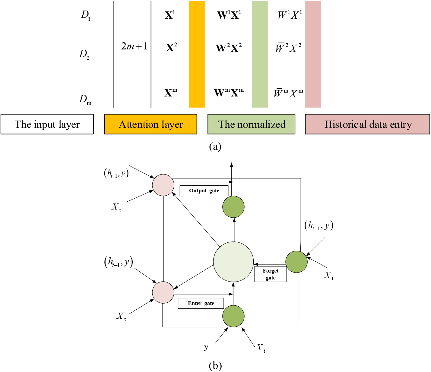

Heuristic algorithms aim to find feasible solutions for combinatorial optimizations within reasonable time and space constraints, providing near-optimal solutions while not guaranteeing feasibility or optimality [23, 24]. These algorithms fall into categories such as traditional, metaheuristic, and super heuristic algorithms. Metaheuristic algorithms, in particular, encompass genetic algorithms, Ant Colony Optimization, and variable neighborhood search algorithms, and they find applications in combinatorial optimizations across various domains [25]. For instance, Hou et al. introduced a model for Building Information Modeling-based big data storage and management [26].

The genetic algorithm belongs to the family of evolutionary algorithms and operates as a metaheuristic natural selection process [27, 28]. Its operation involves several key steps: 1) Coding: Initially, the genetic algorithm requires the determination of the objective function and variables. Subsequently, these variables are encoded, often employing a binary-decimal decoding process, as follows:

$\displaystyle F(b_{i1},b_{i2},b_{il})=R_{i}+\frac{T_{i}-R_{i}}{2^{l}-1}\sum% \limits_{j=1}^{l}{b_{ij}2^{j-1}}$ (17)

In Eq. (17), the notation ( $b_{i1},b_{i2}\ldots,b_{il}$ ) represents the $i$ -th segment of each individual, where each segment has a length of 1 unit. The terms $T_{i}$ and $R_{i}$ refer to the left and right endpoints of the defined domain for the $i$ -th segment component, respectively.

2) The fitness function serves as a metric to assess the fitness of each individual within the population. In this context, the objective function is equivalent to the fitness function [29, 30].

3) The evolutionary process comprises a sequence of fitness-driven genetic operations applied to each individual, a concept known as the “Survival of the Fittest.” These operations encompass selection, crossover, and mutation [31]. To elaborate, selection and crossover fulfill the search function [32, 33, 34], while mutation bolsters the searchability for optimal solutions. Figure 2 depicts the R language code of the classic genetic algorithm.

Figure 2.

R language code of the classic genetic algorithm.

Addressing the challenges of optimizing task-oriented network reconstruction methods in LSTM neural networks, this section employs a genetic algorithm to optimize the initial weights and thresholds of LSTM neural networks. This optimization aims to mitigate limitations, reduce prediction errors, and enhance prediction accuracy. Building upon the preceding discussions, this work delves into the application of the genetic algorithm to optimize LSTM models. The optimization process is outlined in the following steps: 1. Random generation of the initial population. 2. Initialization of the LSTM neural networks. 3. Training of the LSTM neural networks to calculate its total error. 4. Inclusion of the total error in the total fitness function to compute the fitness for each individual. 5. Execution of genetic operations on the current population to generate a new population. 6. If the maximum evolutionary generation is not reached, the current population is used to establish a new LSTM neural network, and Steps 3, 4, and 5 are repeated. 7. Calculation of fitness for all individuals in the current population. 8. Utilization of the remaining data to train the network with the optimal initial weights and thresholds to calculate the network output error. 9. Algorithm termination when the termination conditions are met. The flowchart illustrating the improved LSTM neural networks algorithm is depicted in Fig. 3. This section draws inspiration from the theory of word vectorization (embeddings) in NLP. It involves concatenating the load into vector representations using relevant features to generate new time series data. The Point-In-Time (PIT) historical load is represented through its associated features. Subsequently, the sliding window generates the feature map from the input time series data sequentially. To facilitate subsequent network calculations, the sliding window is configured as follows: width $=$ 16, step size $=$ 1, and unit feature map $=$ 16*16. Meanwhile, the input feature map is organized according to the time series data. The hybrid network model primarily comprises two parts.

Figure 3.

Flowchart of improved LSTM neural networks algorithm.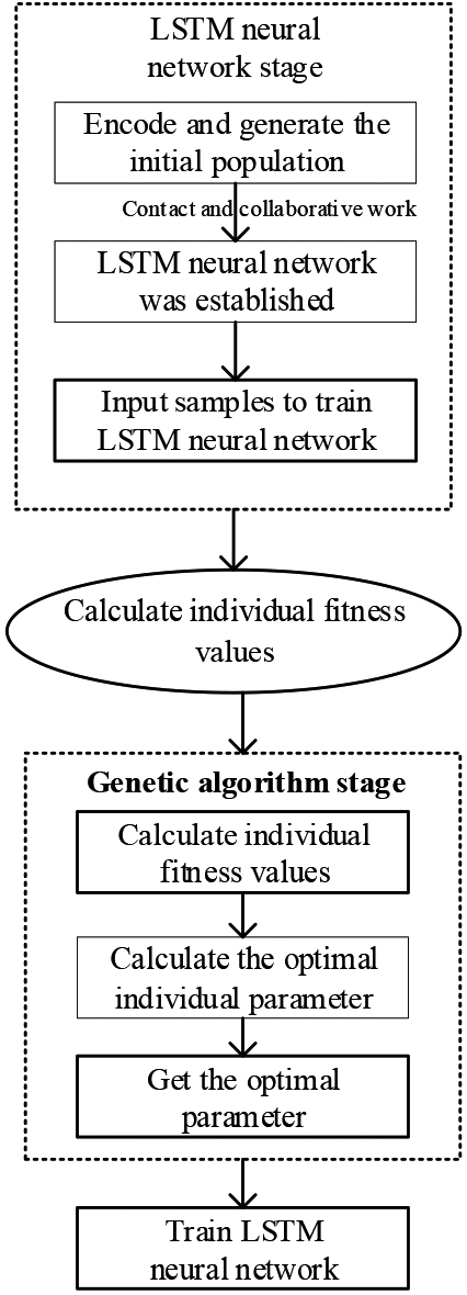

2.3 Network reconstruction based on 1D dynamic equation

Complex systems are often abstracted into complex networks for study. The operation of complex systems typically adheres to specific laws or rules that govern interactions among individual units within the system. When these systems are abstracted into complex networks, the dynamic equation becomes a governing law. A directed graph with $N_{V}$ nodes and $E$ edges can be defined as $G=(V,E)$ , where $V={\{}1,2\ldots,N_{V}{\}}$ represents the set of all nodes in the graph, and $E={\{}e_{jj}{\}}$ represents the set of all edges in the graph. Assuming that the network’s topology is known, each node on the network possesses a state value that changes over time due to the influence of its neighbors and itself. The dynamics of the entire network are described by the functional equation presented in Eq. (18):

$\displaystyle C_{i}(t+1)=f({C_{i}(t)})+\sum\limits_{j=1}^{N_{V}}{w_{ij}}C_{j}(t)$ (18)

In Eq. (18), $C_{i}(t)$ and $C_{j}(t)$ denote the statuses of nodes $i$ and $j$ at time point $t$ , respectively. $C_{i}(t+1)$ represents the status of node $i$ at time point $t+1$ . The parameter $w_{ji}$ represents the weight of the directed edge from node $j$ to node $i$ . The function $f(.)$ represents an affine function that characterizes the activation of the node itself, and its form is shown in Eq. (19).

$\displaystyle f_{i}(x)=\frac{1}{1+e^{-\lambda_{i}x}}$ (19)

In Eq. (19), $f_{i}(x)$ signifies the activation function of node $i$ , and $\lambda_{i}$ denotes the sigmoid parameter of the same node.

The statuses of network nodes evolve over time due to interactions among them. Time series data can be acquired by recording the states of each node at regularly spaced time intervals to capture the dynamics of the network [35, 36].

In a complex network, every node operates under a time-varying dynamic state and continuously engages with other nodes. As a result, a new time series dataset can be generated by recording the individual node states at uniform time intervals. Specifically, $N_{V}$ represents the number of network nodes, while $N_{S}$ indicates the volume of time series data in the dataset. $N_{T}$ stands for the number of PITs in each time series data [37, 38]. The initial step of the proposed algorithm involves initializing the network topology with a random number of edges and weights ranging from $-$ 1 to 1 [39, 40]. The most crucial phase in the network reconstruction process revolves around continuous learning and optimizing the network structure using time series data and optimization algorithms. In particular, the SGD algorithm is employed to optimize and reconstruct the network topology, a decision grounded in theoretical analysis and extensive experimentation. The most effective approach for reconstructing the network using time series data is to treat the time series data as input for the dynamic equation and derive a new series of simulated time series data. More precisely, the new time series data is generated based on the simulated values of the input actual observation time series data at the subsequent PIT. Essentially, the network continues to learn the weight matrix until the state of the generated (simulated) time series data aligns with the real observation time series data at the same PIT, acquiring a weight matrix that closely approximates the real topological structure. Consequently, it becomes imperative to formulate an objective function for assessing the disparity between the simulated time series data and the actual observation time series data. The most commonly employed objective function calculates the difference between the simulated and actual observation values at PIT of $t+1$ based on the real observations at PIT $t$ . Subsequently, this established objective function is employed to gauge the accuracy of network reconstruction. Given the inherent characteristics of time series data, it is not advisable to optimize the network’s weight matrix by designing an objective function that measures the overall error between the real observations and the simulated time series data. In comparison to the traditional Gradient Descent method, the SGD method offers several advantages. For instance, the traditional Gradient Descent method invariably employs an objective function to compute the summation, as depicted in Eq. (20).

$\displaystyle Q(w)=\frac{1}{n}\sum\limits_{i=1}^{n}{Q_{i}}(w)$ (20)

In Eq. (20), $Q(w)$ denotes the loss function, and $w$ is the parameter under estimation aimed at minimizing $Q(w)$ . represents the loss function applied to observation samples within the corresponding dataset. When minimizing the aforementioned loss function, the iterative procedure for the SGD method or Batch Gradient Descent method is illustrated in Eq. (21).

$\displaystyle w:=w-n\nabla Q(w)=w-\eta\sum_{i=1}^{n}Q_{i}(w)$ (21)

Next, the LSTM neural network generates simulated time series data based on the input real-time series data at the next PIT through continuous learning of the weight matrix. At the same PIT, the states of the simulated time series data should align with those of the real-time series data, resulting in a learned weight matrix that closely approximates the actual network topology. Subsequently, an objective function is devised to quantify the disparity between the simulated time series data and the real-time series data. Typically, objective functions hinge on the variance between the simulated value and the actual values at $t+1$ PIT. In the SGD method, solely the gradient of an individual sample is computed instead of the sum of all samples $(Q(w))$ . Equation (22) formulates the estimation method.

$\displaystyle w:=w-\eta\nabla Q_{i}(w)$ (22)

The proposed SGD algorithm operates by systematically scanning the entire training set and updating the parameters based on each individual sample. After several iterative scans, the algorithm converges, and the training samples are shuffled to prevent redundant iterations. Additionally, the proposed SGD algorithm employs an adaptive learning rate to effectively handle noisy samples, thereby ensuring algorithm convergence.

To evaluate the effectiveness of the proposed algorithm, experiments are conducted using GRNs and Social Networks, each containing network nodes ranging from 120 to 200. A typical GRN consists of nodes connected by directed edges with weights falling within the range [ $-$ 1, 1], as illustrated in Fig. 4.

As depicted in Fig. 4, each gene’s state is depicted by a specific numerical value, and the network nodes are interconnected by weighted edges. Consequently, the states of these nodes evolve over time due to interactions through these edges, leading to the generation of dynamic time series data.

2.4 Data sets and evaluation indexes

The GRN and social network datasets are both generated based on the dynamic equation, reflecting the unique characteristics of dynamic systems. These network structures find widespread use in various industries. In social networks, edges are typically undirected, with the presence and absence of edges represented by 1 and 0, respectively, in the adjacency matrix. To accommodate the algorithm’s capacity to reconstruct weighted networks, all undirected edges are substituted with two reverse-directed edges, each pair of which is assigned randomly generated weights. Table 1 provides an overview of the dataset’s fundamental information.

Table 1
Experimental data sets

Type	Volume of networks	Layer volume of nodes	Time series data volume
GRN	5	10	18, 510, 1010, 2010, 30*10
	5	50	110, 510, 1010, 2010, 3010, 5010, 90*10
	1	100	110, 510, 1010, 2010, 3010, 5010, 100*10
Social network	1	34	110, 510, 1010, 2010, 3010, 5010
	1	62	110, 510, 1010, 2010, 3010, 5010, 60*10

Figure 4.

Typical GRN.

In this context, the model error serves as a metric for quantifying the disparity between the actual weight matrix of the network and the weight matrix acquired through time series data learning. The model error index is computed using Eq. (23).

$\displaystyle E_{\text{model}}=\frac{1}{N_{v}^{2}}\sum\limits_{{i=1}}^{N_{V}}{% \sum\limits_{j=1}^{N_{V}}{|{w_{ij}-\hat{w}_{ij}}|}}$ (23)

In Eq. (23), $w_{ij}$ and $\hat{w}_{ij}$ denote the real weight and the learned weight of the edge $<j,i>$ , respectively.

Subsequently, with a learning rate set to 1.2 and a maximum iteration of 1,000, the experimental results, including the model’s error, accuracy, and execution time, are recorded at intervals of 10, 100, 500, 700, and 1,000 iterations. Subsequently, the SGD and the LSM are applied to analyze noisy time series data. Furthermore, a comparative analysis of the reconstruction results obtained by SGD and LSM using a dataset comprising three 50-node networks is conducted, summarizing the strengths and weaknesses of both algorithms.

3. Experimental results and network reconstruction analysis

3.1 Model error test results

Figure 5 displays the model error index obtained from the proposed algorithm across all datasets.

Figure 5.

Test results of algorithm model error ( $n$ represents the data length).

Figure 5 confirms that the proposed algorithm exhibits favorable convergence characteristics across the test datasets. As the number of iterations increases continuously, from 10 to 1,000, the model error exhibits a gradual decrease. However, when dealing with limited time series data, the reduction in model error is more gradual. For instance, in cases where the node count is 50 and the time series data volume is 1*10, the model error remains above 0.2. This indicates that with smaller time series data volumes, the reduction in model error is slower, resulting in a notable disparity between the learned weight matrix and the actual weight matrix. Conversely, when the time series data volume is substantial, the model error diminishes rapidly. The proposed algorithm can reach its minimum error after approximately 50 iterations under these conditions. At this point, the reconstructed weight matrix closely resembles the actual weight matrix, and the algorithm attains convergence swiftly, yielding the optimal solution. Moreover, the model error decreases progressively with increasing iterations. In the case of a Small-World Network, the model error tends to become negligible as the time series data volume surpasses a certain threshold. Additionally, larger networks initially exhibit significant model errors, but these errors can be reduced to nearly zero by augmenting the time series data volume. These experimental results affirm that the model error is challenging to minimize when dealing with limited time series data, resulting in slow error reduction and a noticeable disparity between the learned and actual weight matrices. Conversely, increased time series data volumes enable the algorithm to achieve rapid and effective error reduction, bringing the model error closer to zero. This work explores the intricacies of scaling up networks and the associated challenges in achieving optimal performance. Specifically, when transitioning from a 10-node network to a 100-node network, it is observed that the latter may exhibit increased error rates by the 1000th iteration. This phenomenon can be attributed to incomplete convergence within the specified iteration limit or susceptibility to overfitting issues.

3.2 Analysis of the relationship between algorithm complexity and the number of network nodes and time series data

Figure 6a illustrates the relationship between network node count and algorithm complexity, while Fig. 6b depicts the correlation between network node count and time series data volume.

Figure 6.

Algorithm complexity analysis (x is the number of EXP).

Figure 6a illustrates the relationship between the network node count (100) and algorithm complexity. The execution time of the proposed algorithm increases with the growing time series data volume until it reaches the point of minimum model error. Subsequently, the execution time of the proposed algorithm decreases as the time series data volume continues to rise. Figure 6b depicts the relationship between the network node count and algorithm execution time under the same time series data volume. Notably, the execution time of the proposed algorithm exhibits a linear correlation with the square of the node count. To be specific, the execution time of the algorithm depends on several variables, including the node count, time series data volume, and the number of PITs in each time series data. When the number of samples is fixed, the algorithm’s execution time is positively associated with the square of the node count.

The preceding analysis confirms that the algorithm’s execution time exhibits a linear relationship with the square of the node count. The complexity analysis of the algorithm indicates that its execution time is influenced by several variables, including the number of nodes ( $N_{V}$ ), the time series data volume ( $N_{S}$ ), and the number of PIT in each time series data ( $N_{T}$ ). The algorithm’s complexity can be computed as $O({N_{S}({N_{T}-1})N_{V}^{2}})$ , where $N_{S}({N_{T}-1})$ represents the number of time series data samples. When the sample count is fixed, the algorithm’s execution time is directly proportional to the square of the node count.

3.3 Comparative analysis of algorithms

Figure 7a compares the SGD algorithm and the LSM when the noise Standard Deviation (SD) is set to 0.01, while Fig. 7b illustrates the performance of the SGD algorithm and the LSM when the noise SD is increased to 0.1. In both figures, the x-axis represents the time series data volume, and the y-axis denotes the mean model error.

Figure 7.

Performance comparison between SGD and LSM under the same noise.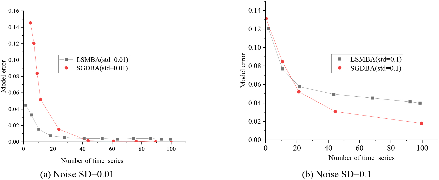

Figure 7 demonstrates an inverse relationship between model error and time series data volume for both the SGD and the LSM. Specifically, when the time series data volume is small, the LSM exhibits a lower error compared to the SGD, but as the time series data volume increases, the LSM’s error surpasses that of the SGD. This analysis indicates that the SGD algorithm benefits from more extensive sample sizes, allowing it to gather more valuable information and adapt its learning rate for improved results. In contrast, the LSM optimizes its performance based on the overall error across the entire sample set, which can sometimes lead to suboptimal results, especially when dealing with significant sample noise. Additionally, the LSM’s performance does not significantly improve with an increased number of samples, making it advantageous for smaller sample sizes.

Figure 8 presents a comparison of the SGD-based and LSM-based models on the same network structure dataset under various noise levels.

Figure 8.

Performance comparison of SGD algorithm and LSM under different noise conditions.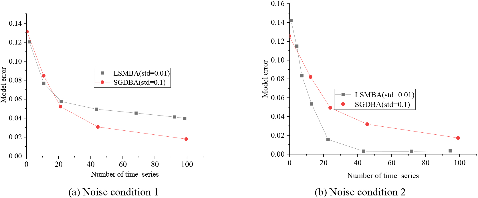

Figure 8 illustrates that both the SGD-based and LSM-based models exhibit a reduction in error as the time series data volume increases. Additionally, Fig. 8a and b reveal that both the SGD-based and LSM-based models display smaller errors when the noise SD is 0.01 compared to when it is 0.1. This sensitivity to noise indicates that the LSM is more susceptible to noise disturbances.

3.4 Discussion

Empirical results demonstrate that SGD outperforms LSM when handling large-sample datasets, showcasing its ability to acquire extensive, high-quality learning information and adaptively adjust learning rates for improved outcomes. However, SGD may exhibit reduced sensitivity to noise, potentially affecting its performance in high-noise environments. In contrast, LSM excels with small-sample datasets by considering overall performance holistically. Nevertheless, its efficacy diminishes with larger datasets as it cannot optimize individual samples. Moreover, as the sample size grows, SGD leverages additional learning information to enhance model generalization. Consequently, LSM typically yields lower errors in scenarios involving small-sample datasets and minimal noise. In comparison, SGD tends to achieve lower errors in situations with large-sample datasets and higher noise levels. These findings underscore the significance of selecting an appropriate optimization algorithm tailored to the data’s characteristics in diverse contexts.

This work thoroughly evaluates an optimization model across various datasets, showcasing its remarkable performance and rapid convergence. However, the model’s runtime demonstrates the correlation with data scale and noise levels. Specifically, in scenarios featuring shorter time series and lower noise levels, the Least-Squares Method proves effective in minimizing model errors. Conversely, as time series length and noise levels escalate, SGD emerges as the more advantageous choice. Consequently, the selection of an optimization algorithm should be guided by a reasonable trade-off between performance and computational complexity, contingent on specific contextual factors.

4. Conclusion

As big data technology continues to advance, complex network theory can now be applied to define increasingly complex systems, including but not limited to GRN, financial systems, ecosystems, and social systems. In practical applications, complex network technology finds utility in various interdisciplinary contexts. The study of complex networks is essential for comprehending the diverse dynamic behaviors exhibited by complex systems and understanding the implications and significance of these network dynamics. This work is pivotal for enhancing our ability to manage complex systems and leveraging networks for the betterment of humanity. Consequently, investigating the underlying complex network models of complex systems through big data technology has become fundamental in the study of dynamic behaviors within these systems. This work focuses on two main aspects: Firstly, it enhances the structure of LSTM neural networks using genetic algorithms within a heuristic framework. This improvement results in the development of a feature-enhanced LSTM network designed for predicting traffic flow data. Additionally, the work addresses data noise by proposing a trend-based noise smoothing scheme. This scheme identifies noise by analyzing historical data and subsequently employs data trends to smooth noisy data. Compared to traditional methods, the smoothed data produced by this scheme is more scientifically sound and reasonable. Besides, the research investigates the challenge of network reconstruction using time series data generated by a one-dimensional dynamic equation. The primary approach involves decomposing time series data into smaller samples and combining adaptive learning rates with the SGD method to optimize the learning process. Model error and the Area Under the Curve are employed to assess the accuracy of the reconstructed network. Experimental results demonstrate that, with proper parameter settings, this algorithm achieves high accuracy and efficiency, making it suitable for reconstructing large-scale networks.

Nonetheless, certain limitations persist in this work. Firstly, the investigation into network reconstruction based on time series data predominantly considers edge weights within the [ $-$ 1, 1] interval. Many real-world community networks, however, may feature substantial edge weights spanning from zero to tens of thousands. The reconstruction of networks under much larger edge weight intervals warrants further exploration. Moreover, the enhancements made to the LSTM model primarily concentrate on improving prediction accuracy, with less attention given to algorithm complexity. This imbalance has led to suboptimal training speeds. Future research endeavors aim to streamline parameters, reduce algorithm complexity, and enhance the efficiency of model training processes.

Footnotes

Funding

This work was supported in part by the Research Projects of Shaanxi Province in Social Development field of Specialized Industrial Innovation Chain under Grant No. 2023-YBSF-397.

References

Dang

, et al. Cost-based multi-parameter logistics routing path optimization algorithm. Mathematical Biosciences, and Engineering. 2019; 16(6): 6975-6989.

Bian

Shao

, et al. Research on multi-feature data routing strategy in deduplication. Scientific Programming. 2020; 2020(4): 1-11.

Puneeth

Kulkarni

. Data aggregation using compressive sensing for energy efficient routing strategy. Procedia Computer Science. 2020; 171: 2242-2251.

Mugunthan

. Novel cluster rotating and routing strategy for software-defined wireless sensor networks. Journal of ISMAC. 2020; 2(3): 140-146.

Erkaymaz

. Resilient backpropagation approach in small-world feed-forward neural network topology based on Newman-Watts algorithm. Neural Computing, and Applications. 2020; 32(11): 32-35.

Liu

Jin

Wang

, et al. PSNet: Reconfigurable network topology design for accelerating parameter server architecture based distributed machine learning. Future Generation Computer Systems. 2020; 106: 320-332.

Kwayu

Kwigizile

Lee

, et al. Discovering latent themes in traffic fatal crash narratives using text mining analytics and network topology. Accident Analysis & Prevention. 2020; 150: 105899.

Yedidsion

Ashur

Banik

, et al. Sensor network topology design and analysis for efficient data gathering by a mobile mule. Algorithmica. 2020; 82(10): 2784-2808.

Safaei

Yeganloo

Akbar

. Robustness on topology reconfiguration of Complex Networks: An entropic approach. Mathematics and Computers in Simulation (MATCOM). 2020; 170(10): 326-329.

10.

Meng

Jiang

Wei

. SCRN: A complex network reconstruction method based on multiple time series. Journal of Circuits, Systems and Computers. 2020; 29(13): 89-96.

11.

Schneider

Loeffler

. Large composite neighborhoods and large-scale benchmark instances for the capacitated location-routing problem. Transportation Science. 2019; 53(1): 301-318.

12.

Misra

Kapadi

Gudi

. Hybrid time-based framework for maritime inventory routing problem. Industrial & Engineering Chemistry Research. 2020; 59(46): 21-27.

13.

Karim

Majumdar

Darabi

, et al. LSTM fully convolutional networks for time series classification. IEEE Access. 2017; 6: 1662-1669.

14.

Khan

Wang

Riaz

, et al. Bidirectional LSTM-RNN-based hybrid deep learning frameworks for univariate time series classification. The Journal of Supercomputing. 2021; 77: 7021-7045.

15.

Khan

Wang

Ngueilbaye

, et al. End-to-end multivariate time series classification via hybrid deep learning architectures. Personal and Ubiquitous Computing. 2020; 1-15.

16.

Khan

Wang

Ngueilbaye

. Attention-based deep gated fully convolutional end-to-end architectures for time series classification. Neural Processing Letters. 2021; 53: 1995-2028.

17.

Erdem

Cubukcu

. Visualizing the road network topology differences of Istanbul city. Environment and Planning A. 2019; 51(4): 827-830.

18.

Wang

. False data injection attacks with incomplete network topology information in smart grid. IEEE Access. 2019; 7: 3656-3664.

19.

Lei

Yang

Fujita

. Random walk-based method to identify essential proteins by integrating network topology and biological characteristics. Knowledge-Based Systems. 2019; 167(5): 53-67.

20.

Anghinoni

Zhao

, et al. Time series trend detection and forecasting using complex network topology analysis. Neural Networks. 2019; 117: 295-306.

21.

Jiang

Chen

Tang

, et al. A physical probabilistic network model for distribution network topology recognition using smart meter data, smart grid. IEEE Transactions on. 2019; 10(6): 6965-6973.

22.

Mallick

Bandyopadhyay

Chakraborty

, et al. Topo2Vec: A novel node embedding generation based on network topology for link prediction. IEEE Transactions on Computational Social Systems. 2019; 6(6): 1306-1317.

23.

Chen

Bowman

Xing

. Detecting and testing altered brain connectivity networks with k-partite network topology. Computational Statistics & Data Analysis. 2019; 141(1): 14-15.

24.

Jayasumana

Paffenroth

Mahindre

, et al. Network topology mapping from partial virtual coordinates and graph geodesics. IEEE/ACM Transactions on Networking. 2019; 27(6): 2405-2417.

25.

Shi

Liao

Tong

, et al. OnionGraph: Hierarchical topology+attribute multivariate network visualization. Visual Informatics. 2020; 4(1): 56-59.

26.

Hou

Wang

Fang

, et al. Edge intelligence for mission-critical 6G services in space-air-ground integrated networks. IEEE Network. 2022; 36(2): 181-189.

27.

Wei

Wang

Fang

, et al. 3U: Joint design of UAV-USV-UUV networks for cooperative target hunting. IEEE Transactions on Vehicular Technology. 2020; 72(3): 4085-4090.

28.

Fang

Wang

Ren

, et al. Age of information in energy harvesting aided massive multiple access networks. IEEE Journal on Selected Areas in Communications. 2022; 40(5): 1441-1456.

29.

Al Mahmud

. A survey on wireless sensor networks architectural model, topology, service, and security. Social Science Electronic Publishing. 2018; 1(1): 18-26.

30.

Cui

Sun

Nie

. Combining network topology with transcriptomic data for identifying radiosensitive gene signatures. Journal of Computational Methods in Sciences and Engineering. 2018; 19(6): 1-15.

31.

Song

Xiao

. Combining time-series evidence: A complex network model based on a visibility graph and belief entropy. Applied Intelligence. 2022; 52(9): 10706-10715.

32.

Chen

Kang

Xing

, et al. Estimating large covariance matrix with network topology for high-dimensional biomedical data. Computational Stats & Data Analysis. 2018; 127(2): 82-95.

33.

Zhang

Liu

. Understanding the mechanisms of brain functions from the angle of synchronization and complex network. Frontiers of Physics. 2022; 17(3): 31504.

34.

Nystrom

Robbins

Deckro

, et al. Simulating attacker and defender strategies within a dynamic game on network topology. Journal of simulation. 2018; 12(4): 307-331.

35.

Zheng

Zhang

. Robustness of cloud manufacturing system based on complex network and multi-agent simulation. Entropy. 2022; 25(1): 45.

36.

Cheng

Huang

Yang

, et al. Silicon photonic switch topologies and routing strategies for disaggregated data centers. IEEE Journal of Selected Topics in Quantum Electronics. 2020; 26(2): 1-10.

37.

Sheikhahmadi

Veisi

Sheikhahmadi

, et al. A multi-attribute method for ranking influential nodes in Complex Networks. Plos One. 2022; 17(11): e0278129.

38.

Huang

Guo

. Integrated sustainable planning of micro-hub network with mixed routing strategy. Computers & Industrial Engineering. 2020; 149(6): 30-49.

39.

Lixia

XIE

Honghong

SUN

Hongyu

, et al. Key node recognition in Complex Networks based on the K-shell method. Journal of Tsinghua University (Science and Technology). 2022; 62(5): 849-861.

40.

Elangovan

Kumanan

. Congestion aware Adaptive Reverse Routing Strategy for Improving QoS in WSN. IOP Conference Series Materials Science and Engineering. 2020; 925(3): 012069.

LSTM network optimization and task network construction based on heuristic algorithm

Abstract

Keywords

1. Introduction

2. Methodology

2.1 Data preprocessing

Table 1 Experimental data sets

3.1 Model error test results

4. Conclusion

Footnotes

Funding

References

Table 1
Experimental data sets