Efficient integrity checks for join queries in the cloud 1

Abstract

Cloud computing is receiving massive interest from users and companies for its convenient support of scalable access to data and services. The variety and diversification of offers by cloud providers allow users to selectively adopt storage and computational services as they best suit their needs, including cost saving considerations. In such an open context, security remains a major concern, as confidentiality and integrity of data and queries over them can be at risk. In this paper, we present efficient techniques to verify the integrity of join queries computed by potentially untrusted cloud providers, while also protecting data and computation confidentiality. Our techniques support joins among multiple data sources and introduce a limited overhead in query computation, enabling also economical savings, as the ability to assess integrity increases the spectrum of offers that can be considered for performing the computation. Formal analysis and experimental evaluations confirm the effectiveness and efficiency of our solutions.

Keywords

Query integrity distributed join semi-join execution verification object

1. Introduction

The competitive pressures are driving the IT sector away from the classical model that assumed the processing and storage of an organization’s data within the internal information system. In fact, more and more often users and organizations use the storage and processing capabilities offered by external cloud providers, which can benefit from economies of scale deriving from the large size of the infrastructure and service catalogue, together with possible access to less expensive resources. Along this line, we can expect a continuous increase in the differentiation of the market for cloud services. For instance, in the area of cloud architectures, interest has emerged on hybrid clouds and on a distinction between storage and computational services. Storage and computational services respond in fact to separate requirements, with distinct profiles. The first should offer reliability for data storage, typically corresponding to cloud providers with high reputation on the market. The second should offer availability of – possibly cheap – computational power, which can be offered by unknown cloud providers. Reputation of the cloud provider is, in this case, less critical, as it is relatively easy to move computation from one provider to another, and the most important parameter becomes the price of the service. An obstacle to a stronger differentiation in the market between storage and computational resources is however represented by the security concerns of users, who can see the involvement of multiple parties in the processing of their information as increasing the risk of confidentiality and integrity violations.

In this paper, we present efficient techniques for verifying the integrity of queries performed by potentially untrusted computational providers, operating over data stored at trusted storage providers. Our techniques aim at controlling in a probabilistic way the behavior of a computational provider that joins data stored at independent trusted storage servers. We address the problem of optimizing integrity controls so to decrease their economic and performance overheads making them suitable to more scenarios and enabling their application with stronger integrity guarantees. In particular, we first introduce an optimization technique that exploits the execution of the join as a semi-join, thus possibly decreasing data communication and performance/economic costs, while leaving unaltered the guarantees offered. We then illustrate another optimization technique that aims at reducing the size of integrity controls. The optimization proposed produces a considerable saving in terms of performance and economic costs. Our analysis also shows that the savings allow an increase in the amount of integrity controls, while still maintaining the same overhead but providing stronger integrity guarantees. In [8] we presented an early version of our approach that here is extended by proposing compact integrity controls. Such integrity controls have a double advantage: they are smaller than the original integrity controls, and they enable the evaluation of many-to-many joins as well as joins involving more than two relations. We then extend the security and performance analysis that evaluates the proposed optimizations, and present the results of an experimental analysis confirming the theoretic results.

The remainder of this paper is organized as follows. Section 2 introduces the basic integrity verification techniques and concepts on which our approach builds. Section 3 illustrates the adaptation of these basic techniques to the semi-join evaluation strategy. Section 4 proposes two optimization techniques, which can be adopted with both regular and semi-join strategies, that limit the overhead of integrity checks. Section 5 analyzes the integrity guarantees provided by the use of the proposed optimizations, evaluating the trade-off between protection and costs. Section 6 shows the advantages, in terms of a reduction in the communication overhead, obtained with the proposed optimizations. Section 7 describes an approach for verifying the integrity of many-to-many joins and joins involving multiple relations. Section 8 presents our experimental analysis. Section 9 discusses related work. Finally, Section 10 concludes the paper.

2. Scenario and basic concepts

We present the basic idea of the approach on which we build our efficient integrity verification techniques. The scenario is characterized by a client that wishes to evaluate a join query over two relations, $B_{l}$ and $B_{r}$ , stored at storage servers $S_{l}$ and $S_{r}$ , respectively, by using a computational server $C_{s}$ . The storage servers are assumed to be trustworthy, while the computational server is not. The query is of the form “select A from $B_{l}$ join $B_{r}$ on $B_{l} . I = B_{r} . I$ where $C_{l}$ and $C_{r}$ and $C_{l r}$ ,” where A is a subset of attributes in $B_{l} \cup B_{r}$ ; I is the set of join attributes; and $C_{l}$ , $C_{r}$ , and $C_{l r}$ are Boolean formulas of conditions over attributes in $B_{l}$ , $B_{r}$ , and $B_{l} \cup B_{r}$ , respectively. The join between relations $B_{l}$ and $B_{r}$ is a one-to-one or a one-to-many join. For simplicity, in the following we assume $B_{l}$ to be the relation on the side “one” and $B_{r}$ to be the relation on the side “many” of a one-to-many join. Typically, in the execution of a query of the form illustrated above, conditions $C_{l}$ and $C_{r}$ are pushed down to each of the storage servers for their evaluation. We assume that, regardless of the degree of the original schema, the relations resulting from the evaluation of $C_{l}$ and $C_{r}$ , denoted L and R, respectively, have schema (I, Attr), where I represents the set of join attributes and Attr represents all the other attributes, both as a unit. Without security concerns, relations L and R can be sent to the computational server that performs the join, evaluates condition $C_{l r}$ , and returns the result to the client. However, since the computational server is not trusted, the proposal in [7]: (i) provides data confidentiality by using encryption on the fly, meaning that the storage servers encrypt their relations L and R (with a key chosen by the client and communicated to $S_{l}$ and $S_{r}$ ) before sending them to the computational server, (ii) provides integrity guarantees by using a combination of the following integrity controls.

Markers: each of the storage servers inserts fake control tuples (markers), not recognizable by the computational server, in the relation to be sent to the computational server. Markers are inserted so to join (i.e., they belong to the result) and to not collide with real join attribute values (to not create spurious joined tuples).

Twins: each of the storage servers duplicates (twins) the tuples in its relation that satisfy a twin condition before sending it to the computational server. The creation of twins is easily controlled by the client by specifying a percentage $p t$ of tuples to be twinned. The twinning condition $C_{twin}$ , operating on the join attribute, is then formulated in such a way to insert the desired number of twin tuples into relations L and R (i.e., $C_{twin} = h_{k} (t [I]) mod ⌊ \frac{1}{p t} ⌋$ , with $h_{k}$ a secure keyed hash-function).

Salts/buckets: used in alternative or in combination to destroy recognizable frequencies of join attribute values in one-to-many joins. Salts consist in salting the encrypted join attribute values at the side “many” of the join (i.e., in R) so that occurrences of a same value become distinct; at the same time, salted replicas are created at the side “one” of the join (i.e., in L) so to create the corresponding matching. Bucketization consists in keeping multiple occurrences of the same (encrypted) value at the side “many” of the join (i.e., in R), but in such a way that all the values have the same number of occurrences. Bucketization can help in reducing the number of salts to be inserted, while possibly requiring insertion of dummy tuples (to fill otherwise not complete buckets).

Fig. 1.

Join computation as a regular join (a) and an example of relations L and R and their extensions with markers, twins, salts and buckets along with the join computed over them (b).

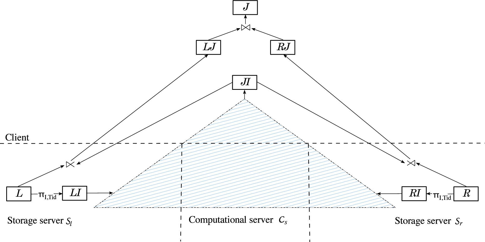
Figure 1(a) illustrates how the join computation works. Each storage server receives in encrypted form: its sub-query, the key to be used to encrypt the sub-query result, and the information necessary to regulate the use of markers, twins, salts and buckets. It then executes the received sub-query (as before), and applies over the resulting relation L (R, resp.) markers, twins, salts and buckets as appropriate, producing a relation $L^{*}$ ( $R^{*}$ , resp.). Relation $L^{*}$ ( $R^{*}$ , resp.) is then encrypted producing relation $L_{k}^{*}$ ( $R_{k}^{*}$ , resp.) that is sent to the computational server. Encrypted relation $L_{k}^{*}$ ( $R_{k}^{*}$ , resp.) contains two encrypted chunks for each tuple: $L_{k}^{*} . I_{k}$ ( $R_{k}^{*} . I_{k}$ , resp.) for the join attribute, and $L_{k}^{*} . {Tuple}_{k}$ ( $R_{k}^{*} . {Tuple}_{k}$ , resp.) for all the other attributes. To avoid inference, a padding schema is used to guarantee that attribute ${Tuple}_{k}$ has the same length for all the tuples in each relation. Note that $L_{k}^{*} . {Tuple}_{k}$ includes also the join attribute as this permits the client to verify the integrity of each tuple singularly taken (i.e., to verify that the computational server has not mixed the values of I and $Attr$ of different tuples). The computational server receives the encrypted relations from the storage servers and computes the natural join between them, returning the result $J_{k}^{*}$ to the client. The client decrypts $J_{k}^{*}$ , and checks whether the tuples have been correctly joined (i.e., $L^{*} . I$ obtained decrypting $L_{k}^{*} . {Tuple}_{k}$ is equal to $R^{*} . I$ obtained decrypting $R_{k}^{*} . {Tuple}_{k}$ ). Note that the use of encryption permits the client to verify also the integrity of individual tuples in the join result. In fact, the computational server does not know the encryption key and hence any (non authorized) modification or insertion of tuples in the join result can be easily identified by the client upon decryption. The client then discards tuples with dummy content, if any. Finally, the client checks integrity by analyzing markers and twins: an integrity violation is detected if an expected marker is missing or a twinned tuple appears solo. Note that the combined use of markers and twins offers strong protection guarantees. In fact, when omitting a large number of tuples from the query results, the probability that the omission goes undetected decreases with respect to the number of markers (e.g., one marker is sufficient to detect that an empty result is not correct), and increases with respect to the number of twins. Also, the probability that the omission of a small number of tuples goes undetected decreases with respect to the number of twins (e.g., a twinned tuple appearing solo is sufficient to detect a non correct result). Figure 1(b) illustrates an example of relations L and R and of their extensions obtained by assuming: the presence of one marker (with value ‘x’ for the join attribute), twinning tuples with values ‘a’ and ‘f’ of the join attribute, and adopting 2 salts and buckets with 2 tuples each. This figure also reports the join result $J^{*}$ obtained by the client decrypting relation $J_{k}^{*}$ received from the computational server. In this example and in the following, to simplify notation, given a value v, notation $\bar{v}$ denotes the twin of v, and notation $v^{'}$ denotes the salted version of value v.

3. Semi-join

The first optimization we illustrate consists in performing the join according to a semi-join strategy. Without security concerns, a semi-join simply implements a join operation by first considering the projection of the join attribute over the stored relations. Only after the join is computed, the join attribute is extended with the other attributes from the source relations to produce the final result. In our distributed setting, semi-joins – while requiring additional data flows – avoid communication of unnecessary tuples to the client and of non-join attributes to the computational server, producing a saving of the total communication costs for selective joins and/or relations with tuples of considerable size (see the experimental results in Section 8). Our approach for executing a semi-join in conjunction with the techniques illustrated in Section 2 is shown in Fig. 2, where the striped triangle corresponds to the process in Fig. 1(a). The execution of the join at the computational server basically works as before: it again receives from the storage servers encrypted relations on which markers, twins, salts and buckets have been applied, computes the join between them, and sends the result to the client. However, in this case:

Fig. 2.

Join computation as a semi-join.

the storage servers do not communicate to the computational server their entire tuples (relations L and R) but rather much slimmer tuples (relations $LI$ and $RI$ ) with only the join attribute and a tuple identifier (both in encrypted form). The tuple identifier ( $Tid$ ) is necessary to keep tuples with the same value for the join attribute in relations $LI$ and $RI$ distinct. It can be either the primary key of L (R, resp.) or an attribute added to L (R, resp.) for the semi-join evaluation.

after checking/cleaning the result of the join (relation $JI$ ), the client asks the storage servers to complete the tuples in the join with the attributes in Attr in their relations (obtaining relations $LJ$ and $RJ$ ), and combines their results.

Note that, while entailing more flows (the regular join process is a part of this), the semi-join execution limits the transfer of non-join attributes, thus reducing the amount of data flows. Note also that, while the storage servers and the client are involved in the execution of some computation to combine tuples, this computation does not entail an actual join execution but rather a simple scan/merge of ordered tuples that then requires limited cost.

Fig. 3.

An example of query evaluation process according to the semi-join strategy: twins on ‘a’ and ‘f’, one marker, two salts, and buckets of size two.

Figure 3 illustrates an example of join computation over relations L and R in Fig. 1(b) according to the semi-join strategy. To simplify the notation, we use Greek letters to denote encrypted data.

4. Limiting the overhead of integrity controls

The adoption of twins, markers, salts and buckets causes communication and computation overhead to the join evaluation process. In this section, we show how to reduce such an overhead while still providing integrity guarantees to the client. Our optimizations aim at limiting (or removing) the use of salts and buckets. For simplicity, in the following discussion, we refer to the execution of the join according to the regular join strategy (Section 2). The optimizations presented in this section can however be applied also with the semi-join strategy, thus reducing the communication and computation overhead in both cases.

4.1. Limiting salts and buckets to twins and markers

The use of salts and buckets on the whole relations L and R causes an increase in the number of tuples within these relations and in the join results. In fact, let s be the number of salts and b be the size of buckets defined by the client. Relation $L^{*}$ includes s copies of each original tuple in L and of each twin. Relation $R^{*}$ instead includes b tuples for each marker (one marker and ( $b - 1$ ) dummy tuples) and between 0 and ( $b - 1$ ) dummy tuples for each value of the join attribute appearing in R and in the twin tuples. Hence, also the join result $J^{*}$ will have b tuples for each marker and between 0 and ( $b - 1$ ) dummy tuples for each original and twinned value of the join attribute. For instance, with respect to the example in Fig. 1(b), the adoption of our techniques causes the presence of six additional tuples in $L^{*}$ , ten additional tuples in $R^{*}$ , and five additional tuples in $J^{*}$ .

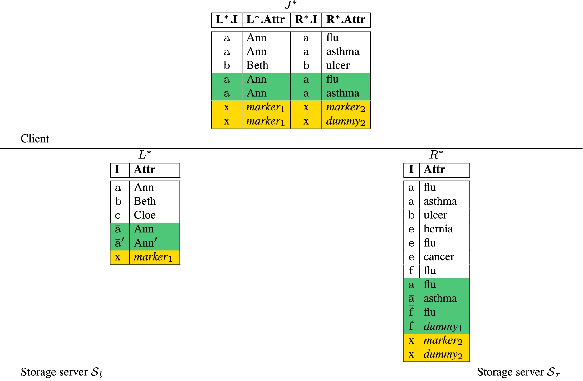
The first optimization we propose aims therefore at limiting the adoption of salts and buckets on twins and markers. Twins and markers (properly bucketized and salted) would form a Verification Object (VO) that can be attached to the original (encrypted) relations. Although the limitation of salts and buckets to twins and markers exposes the frequency distribution of the values of the join attribute in relation R and in the join result, the tuples in the VO have a flat frequency distribution. The computational server then can recognize neither the twin pairs nor the marker tuples. Figure 4 illustrates the extended version of relations L and R in Fig. 1(b) where salts and buckets are limited to twins and markers. This optimization saves three tuples in $L^{*}$ , four tuples in $R^{*}$ , and one tuple in $J^{*}$ .

Fig. 4.

An example of extensions of relations L and R in Fig. 1(b) and their join when salts and buckets are limited to twins and markers.

4.2. Slim twins and slim markers

The second optimization we propose is based on the observation that the integrity check performed by the client only relies on the values of the join attribute of twin and marker tuples. In fact, the replication of the values of the other attributes ( $Attr$ ) of the twinned tuples is not needed and the content of marker tuples is artificial and not of interest for the client. We therefore propose to adopt slim twins and slim markers that differ from (regular) twins and markers in that they store the value of the join attribute only, thus considerably reducing the size of the verification object. Note however that the choice between the adoption, together with slim twins, of slim markers or regular markers should take into consideration the fact that slim markers possibly reduce the resulting protection guarantees (see Section 5).

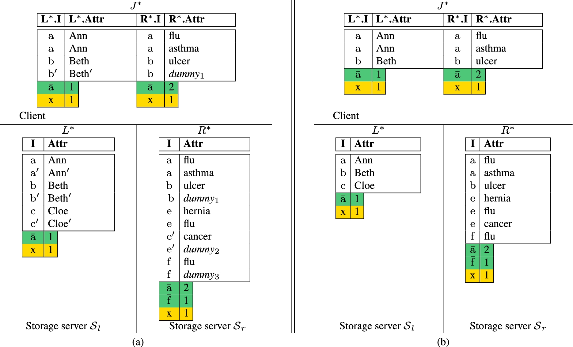
In presence of one-to-many joins, the adoption of slim twins also reduces the number of tuples composing the verification object: one slim tuple with value v for the join attribute can act as a twin for all the original tuples with the same value v for the join attribute. In this case, the slim tuple must include, as the content of attribute $Attr$ , the number of original tuples for which it acts as twin. Note that the size of slim tuples is typically smaller than the size of regular tuples, and slim markers are assumed to have the same size of slim twins so to make them indistinguishable from slim twins. The adoption of slim twins and slim markers reduces the overall size of the verification object, thus saving in communication costs. Due to this difference in the size of the tuples, the computational server can easily identify the tuples forming the verification object. However, the computational server cannot draw any inference from this knowledge because the frequency distribution of the values of the join attribute for the slim twins and slim markers is flat (i.e., each value occurs once), meaning that the computational server cannot exploit the frequency distribution of the join attribute values to identify twin pairs and markers. This also implies that the use of salts and buckets on the verification object is not needed. For the original tuples of a relation, we can still decide whether to use salts and buckets when we need to protect the frequency distribution of the join attribute values of the original tuples. Figures 5(a)–(b) illustrate the extended versions of relations L and R in Fig. 1(b) obtained applying salts and buckets on the original tuples only, and completely departing from salts and buckets, respectively. The verification object includes slim twins for tuples with value ‘a’ and ‘f’ for the join attribute and a slim marker with value ‘x’ for the join attribute. When salts and buckets operate on the original tuples only, we save one tuple in $L^{*}$ , three tuples in $R^{*}$ , and two tuples in $J^{*}$ with respect to the corresponding relations in Fig. 1(b). When departing from salts and buckets, we further save three tuples in $L^{*}$ and in $R^{*}$ , and one tuple in $J^{*}$ . In both cases, the tuples in the verification object are smaller.

Fig. 5.

An example of extensions of relations L and R in Fig. 1(b) and their join adopting slim twins and slim markers with salts and buckets on original tuples only (a) and without salts and buckets (b).

The adoption of slim twins slightly changes the integrity verification process executed by the client. In fact, the client first checks the presence of all the expected markers and then, for each original tuple that satisfies the twin condition, it verifies the existence of one slim twin t in the join result such that the values of attributes $t [L^{*} . I]$ and $t [R^{*} . I]$ are both equal to the values of the twinned tuple. The values stored in $t [L^{*} . Attr]$ and $t [R^{*} . Attr]$ guarantee that the omission of any subset of the original tuples for which t acts as a twin cannot go undetected. In fact, for each slim twin t with frequencies $t [L^{*} . Attr]$ and $t [R^{*} . Attr]$ , the client checks the existence in the join result of $t [L^{*} . Attr] \cdot t [R^{*} . Attr]$ original tuples with the same value for the join attribute. For instance, the slim twin in relation $J^{*}$ in Fig. 5(b) implies the presence of two original tuples with value ‘a’ for the join attribute in the join result.

Although slim twins and slim markers can be used in combination with both regular and semi-join strategies, their effectiveness is higher in a regular join computation than in a semi-join computation. In fact, the semi-join strategy already reduces the size of the tuples in $L^{*}$ and $R^{*}$ (and hence also of twins and markers) since these tuples include the join attribute and the tuple identifier only. The adoption of slim twins would however still reduce the number of tuples in relation R on the side “many” of the join as well as in the join result.

5. Security analysis

We now analyze the integrity guarantees provided by the optimizations illustrated in Sections 3 and 4. In the analysis, we consider a relation $J^{*}$ with f original tuples, t of which satisfy the twin condition, and m markers.

5.1. Semi-join

The semi-join execution strategy leaves unchanged the integrity guarantees offered by the protection techniques in [7]. In fact, the join computed by the computational server relies on the same protection techniques used for the computation of a regular join, and the storage servers are assumed to correctly evaluate the queries received from the client. The probability ℘ that the computational server omits o tuples out of F tuples in relation $J^{*}$ (with $F = f + t + m$ ) without being detected is then the same as regular joins. Probability ℘ is computed as the product between the probability that no marker is omitted ( ${(1 - \frac{o}{F})}^{m}$ ) and the probability that, for each twin pair, either both tuples are omitted or both are preserved ( ${(1 - 2 \frac{o}{F} + 2 {(\frac{o}{F})}^{2})}^{t}$ ), that is, $℘ = {(1 - \frac{o}{F})}^{m} \cdot {(1 - 2 \frac{o}{F} + 2 {(\frac{o}{F})}^{2})}^{t} \approx {(1 - 2 \frac{o}{F})}^{m} \cdot e^{- 2 \frac{t}{F} o}$ . (This probabilistic analysis has also been confirmed by an experimental analysis [7].) Twins formulas show that twins are twice as effective as markers. They however are less effective when a large number of tuples are omitted. In this case, markers are more effective than twins because the greater the number of omissions, the greater the probability of omitting a marker.

5.2. Limiting salts and buckets to the VO and slim twins/markers

The optimizations illustrated in Section 4 may reduce the integrity guarantees provided to the client as they limit the adoption of the protection techniques to reduce the communication overhead. The model we illustrate in the following applies both when limiting salts and buckets to the VO, and when adopting slim twins and slim markers. (The case where slim twins are coupled with regular markers will be analyzed in Section 5.3.)

We examine the probability ℘ that the computational server omits o original tuples without being detected. We build a probabilistic model considering the worst case scenario, assuming that the computational server: (i) recognizes the tuples in the VO (which are easy to recognize because they have a flat frequency distribution when limiting salts and buckets to the VO, and are smaller than the original tuples when adopting slim twins and slim markers), (ii) knows the number m of markers in the VO, (iii) cannot recognize which tuples in the VO are twins and which are markers, or which of the original tuples have been twinned. In the following analysis, we also consider all the tuples with the same value for the join attribute in $J^{*}$ as a single tuple. In fact, if we adopt salts and buckets, the computational server either preserves or omits buckets of tuples in their entirety as omissions of subsets of tuples in a bucket can always be detected. Also the omission of one among the twinned tuples with the same value for the join attribute can be easily detected by checking the corresponding slim twin. The best strategy for the computational server to go undetected is then to either omit or preserve all the tuples with the same value for the join attribute.

If the computational server omits o tuples out of f, it should provide a configuration of the VO consistent with the $(f - o)$ returned tuples to go undetected. In other words, the computational server should omit from the VO all and only the twins of the original tuples removed from the join result. For instance, with reference to the example in Fig. 4, if the computational server omits the tuples with value ‘a’ for the join attribute, it should also remove the tuples with value ‘ $\bar{a}$ ’ from the VO to go undetected. There is only one configuration of the VO that is consistent with the computational server’s omission. This configuration of the VO includes a number of tuples between m (if all the original tuples satisfying the twin condition have been omitted) and $m + t$ (if no original tuple satisfying the twin condition has been omitted). The goal of the computational server is to maximize the probability of finding such a configuration. We model the behavior of the computational server as composed of the following two phases. In the first phase, the computational server determines the number k of tuples in the VO to omit, that is, it tries to guess how many of the o omitted tuples satisfy the twin condition. In the second phase, it chooses the k tuples in the VO that should be omitted, that is, which are the twins of the omitted original tuples.

The goal of the computational server is to determine the number of tuples that would compose the VO if the twins of omitted tuples are also omitted. The probability that the computational server omits k tuples of the t that satisfy the twin condition when omitting o tuples out of the f composing the original join result follows a hypergeometric distribution. The probability $℘_{omit}$ that the VO should contain $(m + t) - k$ tuples for the computational server’s omission to go undetected is then $℘_{omit}$ = $\frac{(\binom{t}{k}) \cdot (\binom{f - t}{o - k})}{(\binom{f}{o})}$ . For instance, the probability that the VO does not miss any tuple, that is, $k = 0$ , is $℘_{omit}$ = $\frac{(\binom{f - t}{o})}{(\binom{f}{o})}$ .

Once the computational server has determined the number k of tuples to remove from the VO, it should decide which tuple in the VO to omit, trying to guess the correct configuration of $(m + t) - k$ tuples to preserve. The number of configurations that omit k out of $(m + t)$ tuples in the VO is $(\binom{m + t}{k})$ . Since only one among these configurations is consistent with the omission of original tuples, the probability $℘_{guess}$ of correctly guessing the k tuples to be omitted is the inverse of this quantity. For instance, if the computational server knows that no tuple satisfying the twin condition has been omitted ( $k = 0$ ), the computational server knows that it should not remove any tuple from the VO. In this case, it is certain of guessing the right configuration for the VO. In fact, $(\binom{m + t}{0}) = 1$ . On the other hand, if all the twins have been omitted (i.e., $k = t$ ), the correct configuration for the VO includes only the m markers. The probability of randomly guessing the right configuration with exactly m tuples choosing among the $m + t$ composing the VO is $\frac{1}{(\binom{m + t}{t})} = \frac{m! \cdot t!}{(m + t)!}$ .

The computational server can estimate the probability ℘ of being undetected as the product between the probabilities of correctly guessing how many tuples ( $℘_{omit}$ ) and which tuples ( $℘_{guess}$ ) should be omitted from the VO (i.e., $℘ = ℘_{omit} \cdot ℘_{guess}$ ). To maximize the chance of not being detected, the computational server will have to choose the strategy that exhibits the greatest value for ℘. To this aim, given the number f of original tuples, t of original tuples having a twin, and m of markers, the computational server is interested in choosing the number k of tuples to omit from the VO that maximizes ℘ and o at the same time.

Fig. 6.

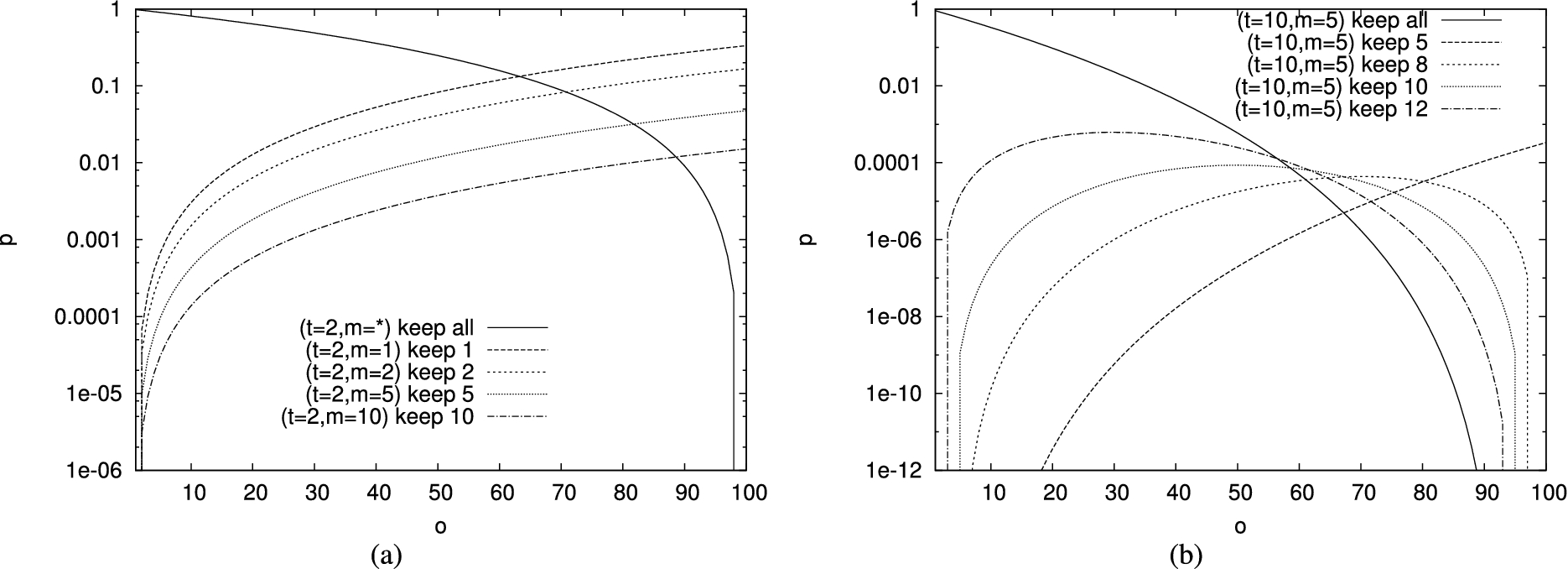
Probability ℘ that the computational server omits o tuples without being detected, considering several strategies, assuming $t = 2$ and $k = t$ (a), and $t = 10$ and $m = 5$ (b).

Figure 6(a) shows the result of the analysis for configurations with $t = 2$ twins and a variable number of markers. The figure compares the “keep all” strategy, where the computational server does not remove any tuple from the VO ( $k = 0$ ), independently from the number of markers ( $m = *$ ), with strategies that keep m tuples in the VO ( $k = t$ ). The computational server will prefer the “keep all” strategy when omitting a few original tuples (less than 60 when $m = 1$ ) as the probability of going undetected is higher. The probability of going undetected however decreases as the number of omissions grows, because it is more likely for the computational server to omit a tuple satisfying the twin condition, as it is visible from the fact that the continuous line in Fig. 6(a) decreases as o grows. As the number of omission grows, the computational server will then naturally prefer to omit also a subset of the tuples in the VO, trying to omit the twins of omitted original tuples. If the computational server omits 2 tuples from the VO (i.e., $k = t = 2$ ), the probability of going undetected grows with the number of omitted original tuples, as visible from the fact that the dashed lines in Fig. 6(a) grow with o. In fact, if the computational server omits more original tuples, it is more likely to remove all the tuples satisfying the twin condition (and then to provide a correct verification object). A higher number of markers naturally reduces the probability for the computational server to guess the correct configuration of the VO, thus offering higher protection. Figure 6(b) considers a configuration characterized by $t = 10$ twins and $m = 5$ markers and compares different omission strategies. Again, the computational server will prefer the “keep all” strategy when omitting a few tuples (less than 55). The cutoff between the “keep all” and the “keep m” strategy that permits the computational server to correctly guess, with higher probability, the number of tuples to omit from the VO moves progressively to the left as the number of tuples kept in the VO grows. Then, as k grows, the computational server more and more prefers the “keep all” strategy (which provides higher values for ℘ in a larger set of configurations). The probability of being undetected when omitting tuples becomes negligible when we consider configurations characterized by a higher number of twins and markers, which we expect to use in real systems.

Fig. 7.

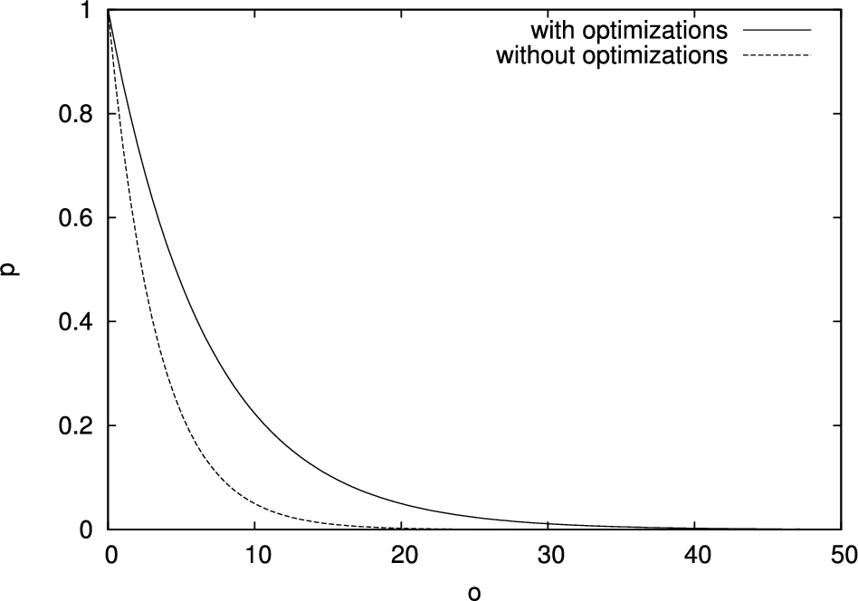
Probability of the omission of o tuples to go undetected when applying the original protection techniques (dashed line) and when adopting optimization techniques that permit to identify the VO (continuous line).

According to the results illustrated above, the computational server will typically prefer the strategy where no tuple in the VO is omitted (“keep all” strategy). In this case, the omission goes undetected if the computational server does not omit any original tuple that has been twinned. The probability that a tuple satisfying the twin condition is omitted from the join result is $\frac{o}{f}$ (the same as each original tuple). Then, the probability ℘ for the computational server to go undetected is equal to $℘ = {(1 - \frac{o}{f})}^{t} \approx e^{- \frac{t}{f} \cdot o}$ . Figure 7 compares the results obtained, fixing f, when no optimization is used and then the computational server cannot identify the tuples composing the VO (“without optimizations” in the figure) with the case where the computational server can determine which tuples represent the VO (“with optimizations” in the figure), assuming $\frac{t}{f} = 15 %$ . We note that limiting salts and buckets to twins and markers, as well as adopting slim twins and slim markers, offers roughly half the protection of applying the original protection techniques. Intuitively, the client can obtain the same protection guarantee by doubling the ratio $\frac{t}{f}$ of twins. Note that since the adoption of slim twins and slim markers reduces the communication overhead caused by twins and markers, the client can double the ratio $\frac{t}{f}$ of twins obtaining the same communication overhead as when no optimization is applied (if the size of slim twins is less than half the size of original tuples). However, even adopting optimization approaches to reduce the overhead caused by integrity verification techniques, the probability that the computational server is not detected when omitting more than 30 tuples is negligible and is independent from the number f of tuples in the original relation. Since the computational server cannot selectively omit tuples from the join result (i.e., it cannot recognize tuples that have a twin), the advantage obtained from the omission of less than 30 tuples does not justify the risk of being detected.

5.3. Slim vs regular markers

When the client decides to rely on slim twins to verify the integrity of join results, it can decide to represent markers as slim tuples or as regular tuples. Slim markers have the advantage of limiting the communication overhead caused by their adoption. Regular markers are indistinguishable from original tuples, thus making it harder for the computational server to identify them. In fact, the number of original tuples is higher than the number of twins and therefore the probability that the computational server correctly guesses regular markers is lower. Note however that, since the join attribute values of markers have a peculiar frequency distribution (their frequency is always one), they are indistinguishable from original tuples only when adopting salts and buckets or in case of one-to-one join operations. In case of one-to-many joins they are instead indistinguishable only from original tuples with a frequency of the values of the join attribute equal to one. The protection offered then depends on the specific instance of relations L and R. To avoid the risk that markers can be easily identified, slim markers should be always adopted (with slim twins) in case of one-to-many joins when salts and buckets are not used.

To decide whether to adopt slim or regular markers, the client can evaluate the trade-off between communication costs and integrity guarantees that each option provides. The communication overhead caused by the adoption of regular markers is due to: the $b - 1$ dummy tuples inserted into R (and then also into J) for each marker to flat their frequency distribution (note that no tuple is inserted into L), and to the larger size of regular tuples. Such an overhead is then equal to $m \cdot (b \cdot ({size}_{J} + {size}_{R}) + {size}_{L} - 3 \cdot {size}_{S})$ , where b is the number of tuples in each bucket, ${size}_{J}$ ( ${size}_{L}$ and ${size}_{R}$ , resp.) is the size of a regular tuple in the join result (in L and in R, resp.), and ${size}_{S}$ is the size of a slim tuple in L and R.

To assess the additional protection provided by the adoption of regular markers, we need to analyze the probability ℘ that an omission of the computational server goes undetected. Similarly to what illustrated in Section 5.2, ℘ is the product of: the probability $℘_{omit}$ that the omission of o regular tuples removes k twinned tuples and no markers, and the probability $℘_{guess}$ to provide a VO consistent with the original tuples. The probability that the computational server omits k tuples of the t that satisfy the twin conditions and no marker when omitting o tuples out of the $f + m$ with regular size follows a multivariate hypergeometric distribution. The probability $℘_{omit}$ is then $℘_{omit} = \frac{(\binom{t}{k}) \cdot (\binom{m}{0}) \cdot (\binom{f - t}{o - k})}{(\binom{f + m}{o})}$ . To provide a VO consistent with the omitted original tuples, the computational server needs to identify the configuration of the VO including $t - k$ tuples where the twins of omitted tuples are not present. Since there exist $(\binom{t}{k})$ configurations omitting k tuples from the VO, $℘_{guess}$ is the inverse of this quantity. 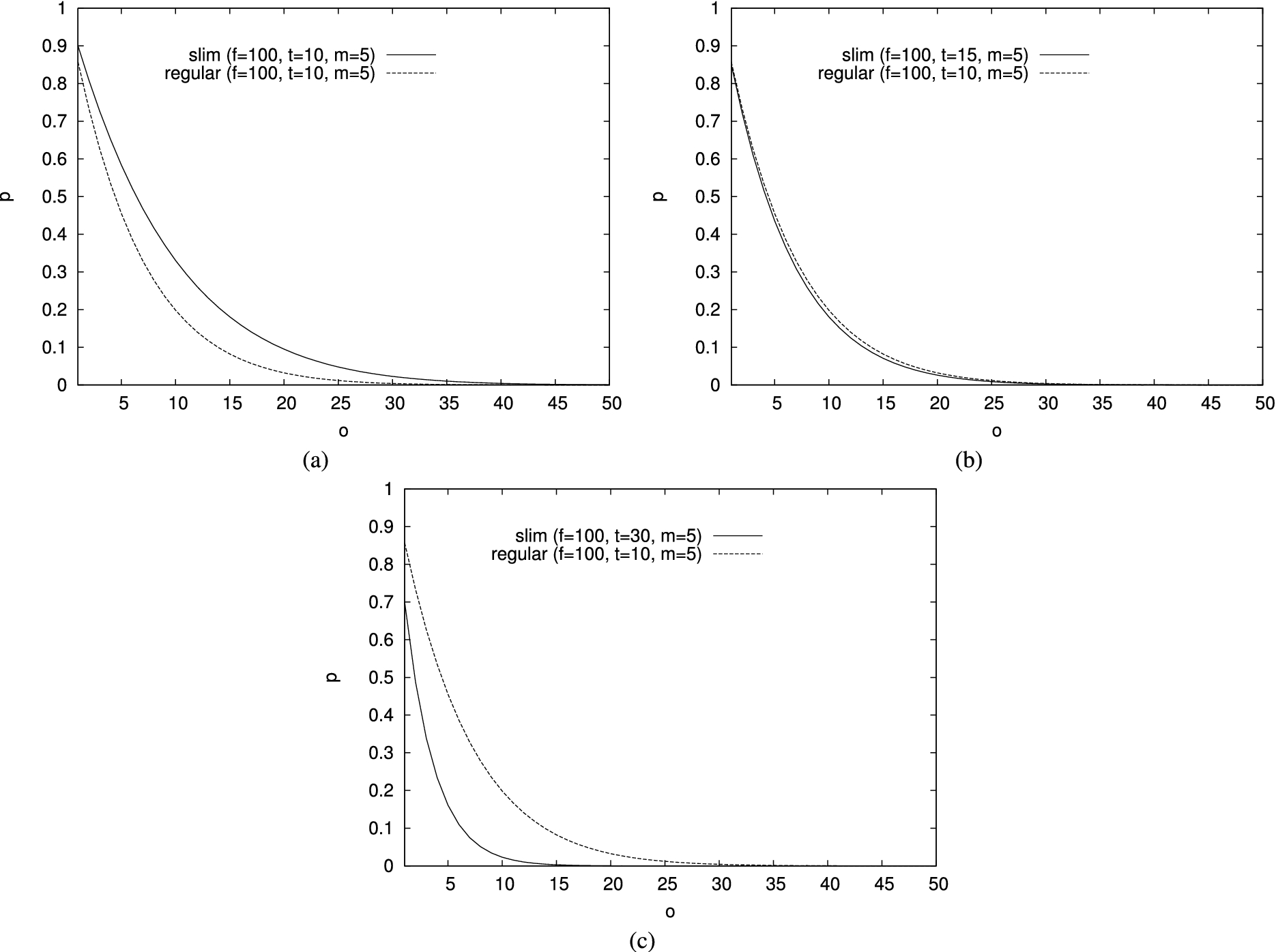The probability of omitting o tuples without being detected is then $℘ = ℘_{omit} \cdot ℘_{guess} = \frac{(\binom{f - t}{o - k})}{(\binom{f + m}{o})}$ .

Fig. 8.

Probability ℘ that the computational server omits o tuples without being detected assuming $m = 5$ and “keep all” strategy, when the ratio between the size of regular and slim tuples is 1:1 (a), 2:1 (b) and 5:1 (c).

Figure 8 compares the probability that an omission goes undetected when adopting slim and regular markers in different configurations, which differ from the relative size of slim and regular tuples. We consider a base configuration characterized by $f = 100$ tuples, $t = 10$ twins, $m = 5$ markers and assume that the computational server adopts the “keep all” strategy, which seems the most promising as discussed in Section 5.2. Figure 8(a) compares the values of ℘ obtained considering slim and regular markers, assuming that slim and regular tuples have the same size (and the computational server can identify the slim tuples composing the VO). In this case, it is immediate to see that regular markers provide higher protection, because they are confused with and are indistinguishable from f original tuples. Slim markers are instead confused with the slim twins in the verification object, and t is usually lower than f. Let us now assume that the client fixes the maximum overhead she is willing to pay for integrity verification (i.e., the maximum overall size of markers and twins). When the size of regular tuples is higher than the size of slim tuples, the adoption of slim markers enables the client to twin a larger subset of original tuples, thus providing higher integrity guarantees. Figure 8(b) compares the results obtained with a base configuration including $f = 100$ tuples, $t = 10$ slim twins, $m = 5$ regular markers, with a configuration with $f = 100$ tuples, $t = 15$ slim twins, $m = 5$ slim markers, obtained assuming that regular tuples are twice as large as slim tuples (i.e., the size of 5 regular tuples is equal to the size of 10 slim tuples, thus allowing the client to use 5 slim markers and 15 slim twins). The figure shows that the integrity guarantees offered by slim twins and slim markers are slightly better than the one obtained with slim twins and regular markers. The protection offered by slim markers increases significantly when the size of regular tuples are five times the size of slim tuples (Fig. 8(c)). Figure 9 confirms that a similar behavior can be observed when the computational server omits t tuples from the VO (i.e., it tries to guess a configuration that includes only markers), considering the same configurations illustrated in Fig. 8. We can then conclude that slim markers are better than regular markers since slim tuples are expected to be much smaller than regular tuples, and, when the overhead for integrity verification is fixed, they also offer higher protection guarantees.

Fig. 9.

Probability ℘ that the computational server omits o tuples without being detected assuming $m = 5$ and “keep m” strategy, when the ratio between the size of regular and slim tuples is 1:1 (a), 2:1 (b) and 5:1 (c).

6. Performance analysis

We now evaluate the performance benefits obtained with the introduction of the semi-join strategy, the use of salts and buckets only on twins and markers, and the adoption of slim twins and slim markers. The performance costs depend on both the computational and communication costs. The computational costs are however dominated by the communication costs. In fact, the computational costs at the client and at the storage servers can be considered limited with respect to the computational costs at the computational server, which however can rely on a high amount of computational resources and on traditional techniques for optimizing join evaluation. In the following, we then focus our analysis first on the communication costs when evaluating a join as a regular join (RegJ) [7] or as a semi-join (SemiJ), according to the process described in Section 3. We then analyze the communication costs obtained when limiting salts and buckets to twins and markers, and when adopting slim twins and slim markers, with and without the use of salts and buckets on the original tuples.

Semi-join vs regular join. This analysis focuses on the amount of data exchanged among the involved parties (i.e., number of tuples transferred multiplied by their size). We first note that both the regular join and the semi-join require a common phase (Phase 1) where there is an exchange of data (tuples) between the storage servers and the computational server and between the computational server and the client. In this phase, regular join and semi-join differ in the size of the tuples transferred among the parties. The semi-join then requires an additional phase (Phase 2) where the client and the storage servers interact to compute the final join result. We analyze each of these two phases in details.

Phase 1 $[S_{l}, S_{r} \to C_{s}; C_{s} \to Client]$ . As already discussed, the only difference between SemiJ and RegJ is the size of the tuples communicated, while the number of tuples in the join operands and in the join result is the same for both strategies. SemiJ requires the transmission of the join attribute and of the tuple identifier only, which are the two attributes forming the schema of relations ${LI}^{*}$ and ${RI}^{*}$ . RegJ requires instead the transmission of all the attributes in $L^{*}$ and $R^{*}$ . If the size of the tuples in $L^{*}$ and $R^{*}$ is higher than the size of the tuples in ${LI}^{*}$ and ${RI}^{*}$ , SemiJ implies a lower communication cost than RegJ. Formally, the amount of data transmitted during this phase is: $\begin{array}{l} RegJ : | L^{*} | \cdot {size}_{L} + | R^{*} | \cdot {size}_{R} + | J^{*} | \cdot ({size}_{L} + {size}_{R}), \\ SemiJ : | {LI}^{*} | \cdot {size}_{IT} + | {RI}^{*} | \cdot {size}_{IT} + | {JI}^{*} | \cdot 2 {size}_{IT}, \end{array}$ where ${size}_{L}$ is the size of the tuples in L, ${size}_{R}$ is the size of the tuples in R, ${size}_{IT} = {size}_{I} + {size}_{Tid}$ is the size of tuples in ${LI}^{*}$ and ${RI}^{*}$ , with ${size}_{I}$ the size of the join attribute I and ${size}_{Tid}$ the size of the tuple identifier $Tid$ . Since ${LI}^{*}$ ( ${RI}^{*}$ and ${JI}^{*}$ , resp.) has the same number of tuples as $L^{*}$ ( $R^{*}$ and $J^{*}$ , resp.), the difference in the communication cost is: $\begin{matrix} | L^{*} | \cdot ({size}_{L} - {size}_{IT}) + | R^{*} | \cdot ({size}_{R} - {size}_{IT}) + | J^{*} | \cdot ({size}_{L} + {size}_{R} - 2 {size}_{IT}) . \end{matrix}$

Phase 2 [ $Client \to S_{l}, S_{r}; S_{l}, S_{r} \to Client$ ]. The number of tuples exchanged between the client and $S_{r}$ is equal to the number of tuples resulting from the join computed by the computational server in the previous phase, after the removal of markers, twins, and dummies (i.e., $| JI | = | RJ |$ ). The number of tuples exchanged between the client and $S_{l}$ depends on the type of join. In case of one-to-one joins, the number of tuples coincides with the number of tuples transmitted from the client to $S_{r}$ (i.e., $| JI | = | LI |$ ). In case of one-to-many joins, the number of tuples is lower since the same tuple in $LI$ (L, resp.) may appear many times in the join result $JI$ (J, resp.). Assuming a uniform distribution of values, the number of different values for the join attribute in $RI$ is $\frac{2 | RI |}{nmax}$ , with nmax the maximum number of occurrences of a value in $RI$ . Given the selectivity σ of the join operation, the number of different values for the join attribute in $JI$ is $σ \cdot \frac{2 | RI |}{nmax}$ , which corresponds to the number of tuples exchanged between the client and $S_{l}$ . The size of the tuples transmitted from the client to each storage server is ${size}_{Tid}$ since the client transmits only the values of the tuple identifier $Tid$ . The size of the tuples transmitted from the storage servers to the client is equal to the size of the tuples in the original relations L and R (i.e., ${size}_{L}$ and ${size}_{R}$ , resp.). Formally, the amount of data exchanged during this phase is: $\begin{array}{rcl} one-to-one join : 2 | JI | \cdot {size}_{Tid} + | JI | \cdot {size}_{L} + | JI | \cdot {size}_{R}; \\ one-to-many join : (| JI | + σ \cdot \frac{2 | RI |}{nmax}) \cdot {size}_{Tid} + σ \cdot \frac{2 | RI |}{nmax} \cdot {size}_{L} + | JI | \cdot {size}_{R} . \end{array}$

By comparing the amount of data transmitted in Phase 2 with the additional amount of data transmitted in Phase 1 caused by the regular join, we note that the semi-join is convenient for relations with large tuples (i.e., ${size}_{IT} ≪ {size}_{L}$ and ${size}_{IT} ≪ {size}_{R}$ ), as also shown by our experimental analysis (Section 8). The advantage of the semi-join with respect to the regular join appears also more evident in case of one-to-many joins where a tuple in the left operand can appear many times in the join result (i.e., $| LJ | \approx σ \cdot \frac{2 | RI |}{nmax} ≪ | JI |$ ). In fact, with the semi-join strategy the client receives each tuple in L that belongs to the final result only once, while it receives many copies of the same tuple when adopting the regular join approach.

Limiting salts and buckets to twins and markers. The analysis consists in evaluating the saving in the number of tuples of relations $L^{*}$ , $R^{*}$ , and $J^{*}$ . We consider each relation in detail.

$L^{*}$ . Since only twin tuples are salted, we save the salted copies of the tuples in L, that is, $(s - 1) \cdot | L |$ tuples.

$R^{*}$ . Since buckets operate only on twins and markers, we save the dummy tuples of the buckets formed with the tuples in R. Since for each value of the join attribute, there is at most one bucket with dummy tuples with, on average, $\frac{b - 1}{2}$ dummy tuples, and there are $\frac{2 | R |}{nmax}$ distinct values for the join attribute (again assuming a uniform distribution of values), we save $\frac{b - 1}{nmax} \cdot | R |$ tuples.

$J^{*}$ . The join result contains the subset of the tuples in $R^{*}$ that combine with the tuples in $L^{*}$ . The number of tuples saved in $J^{*}$ is then a fraction of the number of tuples saved in $R^{*}$ , that is, $σ \cdot \frac{b - 1}{nmax} \cdot | R |$ , where σ is the selectivity of the join operation.

The overall advantage provided by removing salts and buckets from the original tuples is: $(s - 1) \cdot | L | \cdot {size}_{L} + \frac{b - 1}{nmax} \cdot | R | \cdot {size}_{R} + σ \cdot \frac{b - 1}{nmax} \cdot | R | \cdot ({size}_{L} + {size}_{R})$ .

Slim twins and slim markers. Assuming to use salts and buckets on the original tuples of relations $L^{*}$ and $R^{*}$ , the analysis consists in evaluating the saving in the size and in the number of tuples of the verification object of relations $L^{*}$ , $R^{*}$ , and $J^{*}$ . Let $T_{l}$ ( $T_{r}$ , resp.) be the tuples in L (R, resp.) that satisfy the twin condition, and $M_{l}$ ( $M_{r}$ , resp.) be the markers inserted into L (R, resp.). We consider each relation in detail.

$L^{*}$ . No salts are necessary for slim twins, then saving $(s - 1) \cdot | T_{l} |$ tuples. Also, slim twins and slim markers have size ${size}_{S}$ , instead of ${size}_{L}$ , saving $(| T_{l} | + | M_{l} |) \cdot ({size}_{L} - {size}_{S})$ .

$R^{*}$ . Since one slim twin is sufficient for all the tuples with the same value for the join attribute, we need one slim twin in contrast to an average number of $\frac{nmax + 1}{2} + \frac{b - 1}{2}$ twins, with $\frac{nmax + 1}{2}$ the average frequency of join attribute values and $\frac{b - 1}{2}$ the average number of dummy tuples for each original value. Since there are $\frac{2 | T_{r} |}{nmax}$ distinct values for the join attribute (again assuming a uniform distribution of values), we save $(\frac{nmax + 1}{2} + \frac{b - 1}{2} - 1) \cdot \frac{2 | T_{r} |}{nmax} = \frac{| T_{r} | (nmax + b - 2)}{nmax}$ tuples. We also save $b - 1$ tuples for each slim marker. Also, slim twins and slim markers have size ${size}_{S}$ , instead of ${size}_{R}$ , saving $(\frac{| T_{r} | (nmax + b - 2)}{nmax} + | M_{r} |) \cdot ({size}_{R} - {size}_{S})$ .

$J^{*}$ . The join result contains the subset of the tuples in $R^{*}$ that combine with the tuples in $L^{*}$ . Except for markers, the number of tuples saved in $J^{*}$ is then a fraction of the number of tuples saved in $R^{*}$ , that is $σ \cdot \frac{| T_{r} | (nmax + b - 2)}{nmax}$ . Also, slim twins and slim markers have size $2 {size}_{S}$ , then saving $(σ \cdot \frac{| T_{r} | (nmax + b - 2)}{nmax} + | M_{r} |) \cdot ({size}_{L} + {size}_{R} - 2 {size}_{S})$ .

The advantage provided by the adoption of slim twins and slim markers is considerable and is obtained as the sum of the three components above.

Note that when we use slim twins and slim markers completely departing from salts and buckets, the saving in the communication cost corresponds to the sum of the savings obtained when limiting salts and buckets to the verification object and when salts and buckets are only applied to the original tuples of relations $L^{*}$ and $R^{*}$ in combination with slim twins and slim markers. In fact, these two optimizations operate on disjoint subsets of tuples (i.e., the original tuples and the verification object, respectively).

7. Multiple joins

The semi-join approach and the optimizations on the use of salts, buckets, twin, and markers illustrated in the previous sections only support one-to-one and one-to-many joins involving two relations. We now extend our integrity verification techniques to allow the client to delegate many-to-many joins and joins among more than two relations to the computational server.

7.1. Many-to-many joins

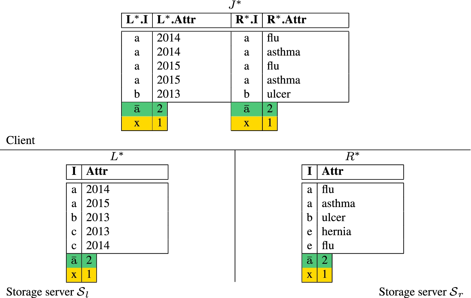
Twins, markers, salts and buckets do not support the evaluation of many-to-many joins because salts and buckets can hide the frequency distribution of the join attribute values only on one of the sides of the join operation, but not on both (thus possibly enabling the computational server to identify twin pairs and markers). With the adoption of slim twins and slim markers, however, the join between the tuples composing the VO of the two relations is always a one-to-one join, independently from the cardinality characterizing the join between the original tuples in L and R (see Section 4.2). Hence, assuming to completely depart from salts and buckets, the computational server cannot exploit the frequency distribution of the join attribute values in the join result to identify twin pairs and markers (i.e., slim twins and slim markers enable the evaluation of many-to-many joins). Figure 10 illustrates two relations and their extended version where slim twins are defined on tuples with join attribute equal to ‘a’, and there is one slim marker with value ‘x’ for the join attribute. Note that even if ‘a’ appears twice in both $L^{*}$ and $R^{*}$ , there is one slim twin representing it in both relations. The figure also illustrates the result of the many-to-many join between $L^{*}$ and $R^{*}$ , which includes one slim twin and one slim marker.

To verify the completeness of the join result, the client needs to check: the presence of all the expected markers (in our example, a tuple with value ‘x’ for the join attribute); for each original tuple satisfying the twin condition, the presence of one slim twin with the same value for the join attribute; and for each slim twin t, the presence of $t [L^{*} . Attr] \cdot t [R^{*} . Attr]$ original tuples with value $t [I]$ for the join attribute. With reference to the example in Fig. 10, the client should check the presence of: one marker with value ‘x’; one slim twin with value ‘a’; and $2 \cdot 2 = 4$ tuples with value ‘a’.

Fig. 10.

An example of many-to-many join between relations extended with slim twins and slim markers.

7.2. Joins among multiple relations

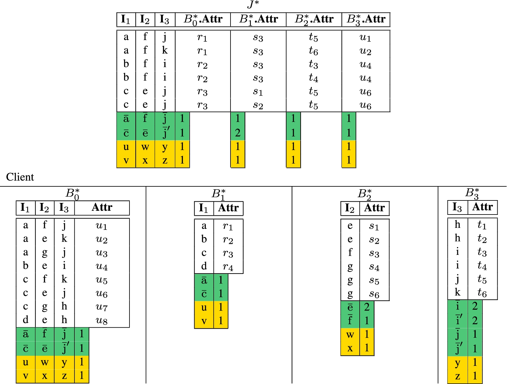
Before illustrating how to support joins among multiple relations, we observe that the case when, for every relation, the attribute participating in the joins is always the same, we can apply the solution illustrated in Section 4.2. When relations participate in different joins with different attributes, an adaptation is instead necessary. In the following discussion, we consider star join operations involving an arbitrary number of relations such that one of the relations appears in all the joins with the others. For instance, the join among relations $B_{0}$ , $B_{1}$ , $B_{2}$ , and $B_{3}$ in Fig. 11 is a star join, where relation $B_{0}$ is at the center of the star and is involved in the join with each of the other relations. To verify the integrity of star join queries, we need to guarantee that the amount of integrity controls, in terms of number of slim markers and slim twins expected in the join result, is not affected by the number of relations (i.e., the evaluation of additional join conditions should not remove the control tuples), and that the computational server is not able to identify twin pairs and marker tuples. To fix ideas, and make the discussion clear, consider a set ${B_{0}, \dots, B_{n}}$ of relations, where $B_{0}$ is the relation at the center of the star and ${I_{1}, \dots, I_{n}}$ are the join attributes, with $I_{i}$ the join attribute in relations $B_{i}$ and $B_{0}$ .

The number of slim twins and slim markers in the join result can be reduced due to the presence of a higher number of operands in the join. Indeed, each additional relation implies the evaluation of an additional (join) condition that the tuples in the join result should satisfy. To guarantee that the join result includes the number of slim markers and the percentage of slim twins expected by the client, we then need to coordinate the generation of markers and the definition of twin conditions among all the storage servers. In the following, we illustrate how markers and twins are generated, and then describe how a star join is performed.

Markers. The presence of all the expected markers in the join result is guaranteed by forcing the storage server storing relation $B_{0}$ to use, for each join attribute $I_{i}$ , the same values as the storage server holding the corresponding relation $B_{i}$ , with no replication. Note that it is not important how the attribute values are combined in the markers of relation $B_{0}$ as any combination guarantees the presence of all the expected markers in the join result. For instance, consider relations $B_{0}$ , $B_{1}$ , $B_{2}$ , and $B_{3}$ in Fig. 11 and assume that the client wants to guarantee the presence of two markers in the join result. Two markers are then inserted into $B_{1}$ (‘u’ and ‘v’), $B_{2}$ (‘w’ and ‘x’), and $B_{3}$ (‘y’ and ‘z’). The storage server storing $B_{0}$ is requested to insert two markers with values ‘u’ and ‘v’ for $I_{1}$ , ‘w’ and ‘x’ for $I_{2}$ , and ‘y’ and ‘z’ for $I_{3}$ . In the figure, $B_{0}$ includes tuples $⟨ u, w, y, 1 ⟩$ and $⟨ v, x, z, 1 ⟩$ . Note however that also tuples $⟨ u, x, y, 1 ⟩$ and $⟨ v, w, z, 1 ⟩$ would work. In fact, it is sufficient that attribute $I_{1}$ ( $I_{2}$ and $I_{3}$ ) in $B_{0}$ assumes, for marker tuples, the same values as $I_{1}$ in $B_{1}$ ( $I_{2}$ in $B_{2}$ and $I_{3}$ in $B_{3}$ ) with no replication to guarantee the presence of the markers in the join result.

Fig. 11.

An example of four relations, their extensions with slim twins and slim markers, and the result of their join.

Twins. The presence of twins in the join result is obtained applying the same twin condition on all the relations sharing a common join attribute (i.e., the same twin condition on attribute $I_{i}$ , $i = 1, \dots, n$ , is applied to $B_{0}$ and $B_{i}$ ). This guarantees that the storage servers storing $B_{0}$ and $B_{i}$ , $i = 1, \dots, n$ , insert twins with the same values for the join attribute $I_{i}$ (i.e., the twins satisfy the join condition between $B_{0}$ and $B_{i}$ ). To guarantee that the twin tuples inserted into each relation are preserved in the computation of the join, the twin condition operating on relation $B_{0}$ should therefore be the conjunction of the twin conditions operating on relations $B_{1}, \dots, B_{n}$ . For instance, consider the relations in Fig. 11, and assume that the client twins the tuples in $B_{1}$ with value ‘a’ and ‘c’ for $I_{1}$ , values ‘e’ and ‘f’ for $I_{2}$ in $B_{2}$ , and values ‘i’ and ‘j’ for $I_{3}$ in $B_{3}$ . The twins corresponding to tuples that satisfy only a subset of the twin conditions (e.g., tuple $⟨ a, e, k, u_{2} ⟩$ ) will not belong to the join result, since there will not be twins with the same values for the join attributes in $B_{i}$ , $i = 1, \dots, n$ (e.g., there cannot be a tuple in $B_{3}^{*}$ with value $\bar{k}$ for $I_{3}$ ). Hence, twinning them would be useless for the final check by the client. Since the client has knowledge neither of the values of the join attribute populating each relation nor of the combination of values in $B_{0}$ , the definition of n twin conditions operating on $I_{i}$ , $i = 1, \dots, n$ , each duplicating a percentage $p t$ of the tuples in $B_{i}$ , $i = 1, \dots, n$ , does not provide any guarantee on the fact that the same percentage of tuples will be twinned in $B_{0}$ . Assuming that the values of the attributes participating in the different join operations are independent (i.e., there is no correlation among their values), the percentage of tuples in $B_{0}$ that satisfies all the twin conditions will be $p t_{1} \cdot p t_{2} \cdot \dots \cdot p t_{n}$ , where $p t_{i}$ is the percentage of tuples satisfying the twin condition on $I_{i}$ in $B_{i}$ , $i = 1, \dots, n$ . To obtain a given percentage $p t$ of twins in the final result, the client should then choose $p t_{1}, \dots, p t_{n}$ in such a way that their product is equal to $p t$ . Note that the percentage of twins can be different in each relation. For instance, with reference to our example, to obtain 12.5% of twins in the join result, the client could decide to twin 50% of the tuples in $B_{1}$ , $B_{2}$ , and $B_{3}$ , or to twin 25% of the tuples in $B_{1}$ , 50% in $B_{2}$ and all the tuples in $B_{3}$ .

We have shown that with slim twins and slim markers the frequency distribution of the join attribute values in the verification object is flat (Section 4.2). However, when joining multiple relations, the same value for a join attribute may have multiple occurrences. In particular, relation $B_{0}$ may have multiple occurrences of the same value for a join attribute $I_{i}$ . Consider, as an example, the original tuples in relation $B_{0}$ in Fig. 11 and assume that tuples with value ‘a’ or ‘c’ for $I_{1}$ , ‘e’ or ‘f’ for $I_{2}$ , and ‘i’ or ‘j’ for $I_{3}$ satisfy the twin condition. The first and sixth original tuples in $B_{0}$ satisfy the twin condition, thus generating two twin tuples with values $⟨ \bar{a}, \bar{f}, \bar{j}, 1 ⟩$ and $⟨ \bar{c}, \bar{e}, \bar{j}, 1 ⟩$ , respectively. It is easy to see that value ‘j’ appears twice. By analyzing the frequency distribution of join attribute values appearing in the slim twins of relation $B_{0}$ , the computational server can then recognize twin pairs and/or markers. With respect to the previous example, the computational server can easily infer that tuple $⟨ b, e, i, u_{4} ⟩$ has not been twinned because the value of attribute $I_{3}$ has one occurrence while the two slim twins have the same value for attribute $I_{3}$ . (Note that the twins in the relations at the edge of the star will never have more than one occurrence for each value of the join attribute.) To avoid this kind of inferences, we must flatten the number of occurrences of join attribute values in the VO of relation $B_{0}$ . We then propose to apply salts on slim twins as follows. Given the maximum number nmax of occurrences of a value of join attribute $I_{i}$ , $i = 1, \dots, n$ , in the twins of $B_{0}$ , the storage server storing $B_{i}$ , $i = 1, \dots, n$ , generates nmax salted replicas of each of its slim twins. The storage server storing $B_{0}$ instead applies a different salt to each occurrence of the same value in $I_{i}$ , $i = 1, \dots, n$ . For instance, with reference to the example in Fig. 11, the maximum number of occurrences of twinned values of $I_{1}$ and $I_{2}$ is one (no salt is needed), while it is two for $I_{3}$ . Relation $B_{3}^{*}$ then duplicates all its slim twins, applying a salt to one of the replicas, while $B_{0}^{*}$ makes the two copies of ‘ $\bar{j}$ ’ different by adopting a salt. Note that all the replicas, with different salts, of the same join attribute value are associated with the actual number of occurrences of the value in the original relation as it is necessary to enable the client to verify the completeness of the join result.

Join process. The join operation is evaluated according to the strategy illustrated in Section 2 (or the semi-join strategy illustrated in Section 3). Each storage server receives in encrypted form: its sub-query, the key to be used to encrypt the sub-query result, and the information necessary to regulate the use of slim markers, slim twins, and salts. It then executes the received sub-query, inserts slim markers, generates slim twins for the tuples satisfying the twin condition, applies salts, and encrypts the relation obtained. All the storage servers send their encrypted relations to the computational server, which computes the join result and sends it to the client. The client decrypts the relation received from the computational server and verifies its integrity. To this aim, it checks whether the tuples have been correctly joined (i.e., if the plaintext values of the join attributes satisfy the join conditions), if all the expected markers belong to the join result, and if slim twins are consistent with original tuples. Slim twins are consistent with the join result if: (1) for each original tuple satisfying the conjunction of all the twin conditions there is a slim twin with the same combination of values for the join attributes; and (2) for each slim twin t there are $t [B_{0} . Attr] \cdot \dots \cdot t [B_{n} . Attr]$ original tuples with the same combination of values for the join attributes. For instance, with reference to the example in Fig. 11, the client verifies the presence of two markers with values ‘u’ and ‘v’ for $I_{1}$ , ‘w’ and ‘x’ for $I_{2}$ , and ‘y’ and ‘z’ for $I_{3}$ . It also verifies, based on slim twins, the presence of one original tuple with values $⟨ a, f, j ⟩$ and two with values $⟨ c, e, j ⟩$ .

8. Experimental results

In this section, we discuss the benefits obtained when adopting the semi-join evaluation strategy, limiting the adoption of salts and buckets to twins and markers, and using slim twins and slim markers.

8.1. Regular join vs semi-join

To assess the performance and economic advantage of the semi-join with respect to the regular join strategy we implemented a prototype enforcing our protection techniques and run a set of experiments. We used for the computational server a machine with 2 Intel Xeon Quad 2.0 GHz, 12 GB RAM. The client machine and the storage servers were standard PCs running an Intel Core 2 Duo CPU at 2.4 GHz, with 4 GB RAM, connected to the computational server through a WAN connection with a 4 Mbps throughput. The values reported in the remainder of this sections are the average over six runs.

Response time. A first set of experiments was dedicated to compare the response time of the regular join and the semi-join strategies. The experiments also evaluated the impact of latency on the computation, comparing the response times for queries over local networks (local client configuration) with those obtained with a client residing on a PC at a distance of 1,000 km connected through a shared channel that in tests demonstrated to offer a sustained throughput near to 80 Mbit/s (remote client configuration). The experiments used a synthetic database with two relations, each with a number of tuples between $10^{4}$ and $10^{6}$ , with size equal to 30 and 2,000 bytes. We computed one-to-one joins between these relations, using 500 markers and 10% of twins. The results of these experiments are reported in Figs 12(a)–(b).

The results confirm that the use of semi-join (SemiJ, in the figure) gives an advantage with respect to regular join (RegJ, in the figure) when the tuples have a large size, whereas the advantage becomes negligible when executing a join over compact tuples. This is consistent with the structure of the semi-join computation, which increases the number of exchanges between the different parties, but limits the transfer of non-join attributes. When the tuples are large, the benefit from the reduced transfer of the additional attributes compensates the increased number of operations, whereas for compact tuples this benefit is limited. The experiments also show that the impact of latency is modest, as the comparison between local client and remote client configurations of the response times for the same query shows a limited advantage for the local client scenario, consistent with the limited difference in available bandwidth. The results obtained also confirm the scalability of the technique, which can be applied over large relations (up to 2 GB in each relation in our experiments) with millions of tuples without a significant overhead.

Fig. 12.

Response time for regular join and semi-join considering tuples of 30 bytes (a) and tuples of 2,000 bytes (b).

Economic analysis. Besides the response time perceived by the user, the choice between regular and semi-join needs to take into consideration also the economic cost of each alternative. We focused on evaluating the economic advantage of the availability of the semi-join, besides regular join, strategy when executing queries [19]. In fact, in many situations the semi-join approach can be less expensive, since it entails smaller flows of information among the parties.

In our analysis, we assumed economic costs varying in line with available solutions (e.g., Amazon S3 and EC2, Windows Azure, GoGrid), number of tuples to reflect realistic query plans, and reasonable numbers for twins and markers. In particular, we considered the following parameters: (i) cost of transferring data out of each storage server (from 0.00 to 0.30 USD per GB), of the computational server (from 0.00 to 0.10 USD per GB), and of the client (from 0.00 to 1.00 USD per GB); (ii) cost of transferring data to the client (from 0.00 to 1.00 USD per GB);2

We did not consider the cost of input data for the storage and computational servers since all the price lists we accessed let in-bound traffic be free.

(iii) cost of CPU usage for each storage server (from 0.05 to 2.50 USD per hour), for the computational server (from 0.00 to 0.85 USD per hour), and for the client (from 1.00 to 4.00 USD per hour); (iv) bandwidth of the channel reaching the client (from 4 to 80 Mbit/s); (v) size

{size}_{IT} = {size}_{I} + {size}_{Tid}

of the join attribute and the tuple identifier (from 1 to 100 bytes); (vi) number of tuples in L (from 10 to 1,000) and the size of the other attributes

{size}_{L} - {size}_{IT}

(from 1 to 300 bytes); (vii) number of tuples in R (from 10 to 10,000) and the size of the other attributes

{size}_{R} - {size}_{IT}

(from 1 to 200 bytes); (viii) number m of markers (from 0 to 50); (ix) percentage

\frac{t}{f}

of twins (from 0 to 0.30); (x) number s of salts (from 1 to 100); (xi) maximum number nmax of occurrences of a value in R.I (from 1 to 100); (xii) selectivity σ of the join operation (from 0.30 to 1.00). Similarly to what is usually done in finance and economics to compare alternative strategies in systems whose behavior is driven by a large number of parameters assuming values following a probability distribution, we used a Monte Carlo method to generate 2,000 simulations varying the parameters above and, for each simulation, we evaluated the cost of executing a join operation as a regular and as a semi-join.

Fig. 13.

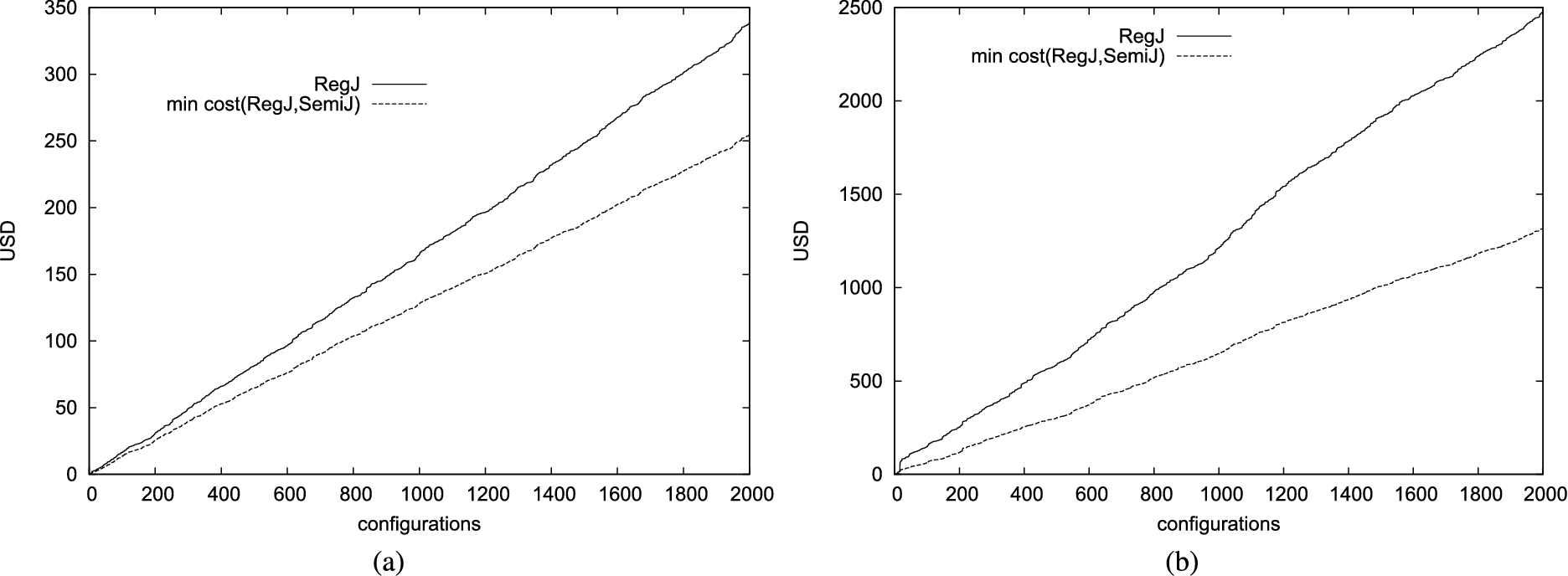
Total economic cost of executing 2,000 one-to-one (a) and 2,000 one-to-many (b) join queries as a regular join or as the less expensive between regular and semi-join.

We compared the cost of evaluating 2,000 one-to-one and 2,000 one-to-many join queries with (and without resp.) the availability of the semi-join technique for query evaluation. We assume that the query optimizer can assess which of the two strategies (i.e., RegJ, SemiJ) is less expensive for each query. Figures 13(a)–(b) illustrate the total costs as the number of query grows for the two scenarios, considering one-to-one and one-to-many queries, respectively. As visible in the figure, if all the queries are evaluated adopting the regular join approach, the total cost (continuous line) reaches higher values than with the availability of the semi-join approach (dotted line). This trend is more visible for one-to-many joins, where the total cost reached when all the queries are evaluated as regular joins is 2,475 USD while with the availability of the semi-join approach it remains at 1,321 USD, with a total saving of 1,154 USD (corresponding to 46,85%). In fact, out of the 2,000 one-to-many queries, 1,784 were evaluated as semi-joins, while for the remaining 216 the regular join solution was cheaper. For one-to-one joins, as expected, the total saving is lower (24.77%) since half of the 2,000 queries considered are cheaper when evaluated as regular joins.

8.2. Limiting salts and buckets to the VO

A second set of experiments was dedicated to the analysis of the use of salts and buckets on twins and markers only. The experiments considered a one-to-many join, evaluated as a regular join, over a synthetic database. We considered different configurations obtained varying different parameters starting from a base scenario. The base scenarios is characterized by $10^{6}$ tuples of 1,000 bytes in L, $10^{8}$ tuples of 100 bytes in R, $20 %$ selectivity σ of the join, 20 markers, and $20 %$ of twins. The number of salts adopted is equal to $⌈ \sqrt{nmax} ⌉$ , which is the value causing the minimum overhead in join evaluation [7]. The frequency of the values for the join attribute in relation R follows a Zipf probability distribution with parameter γ between 0 and 1, where lower values of γ correspond to skewed distributions with more occurrences of fewer values.

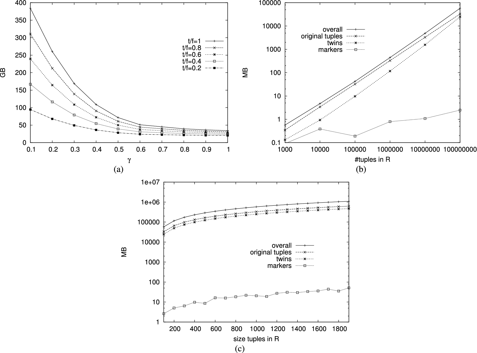
We first analyzed the scalability of the adoption of salts and buckets on the VO only. To this purpose, we measured the size (in MB) of the relations transmitted among the parties. In fact, the communication cost represents the dominating factor and directly depends on the size of the exchanged relations. Figure 14(a) compares the size in GB of $R^{*} + L^{*} + J^{*}$ obtained with the adoption of a different percentage of twins, varying the parameter γ of the Zipf distribution. We note that the size of the relations exchanged is inversely proportional to γ. When γ is low, the overhead caused by the adoption of our approach is higher, since it is necessary to adopt a higher number of salts and larger buckets to flatten the frequency distribution of very frequent values in the VO. The approach instead proves to scale well with the percentage of twins. Figures 14(b)–(c) illustrate how the size of the original relations, twins, and markers grows with the number of tuples in the operand relations (the number of tuples in L is 1/100 the number of tuples in R) and with their size (the size of tuples in L is 10 times the size of tuples in R). The two figures confirm the scalability of the approach. In fact, the size of the verification object, and then also of the extended relations, linearly grows with the number of tuples of the original relations and with their size. The two figures also confirm that most of the traffic generated among the parties is due to original tuples.

Fig. 14.

Size of extended relations when limiting salts and buckets to the VO, varying γ and the percentage of twins (a), the number of tuples in R (b), and the size of tuples in R (c).

The overhead caused by the adoption of the integrity verification techniques illustrated in Section 2 is represented by the set, denoted ${VO}_{b}$ , of tuples including: twins, markers, dummy tuples in $R^{*}$ , and salted copies of tuples in $L^{*}$ . When limiting salts and buckets to the VO, the overhead is represented by the set, denoted ${VO}_{l}$ , of tuples including twins and markers, properly salted and bucketized. To assess the advantage provided by limiting salts and buckets to the VO, we analyzed the ratio $\frac{| {VO}_{l} |}{| {VO}_{b} |}$ between the number of tuples in ${VO}_{l}$ and in ${VO}_{b}$ . Value 1 for the ratio means that the number of tuples inserted for integrity verification is the same in both cases, while a value lower than 1 denotes a saving obtained when limiting salts and buckets to the VO. Figure 15(a) compares the ratio $\frac{| {VO}_{l} |}{| {VO}_{b} |}$ obtained when adopting different percentages of twins, varying the parameter γ of the Zipf distribution. The figure shows that limiting salts and buckets to the VO provides higher benefits when the frequency distribution of the values of the join attribute is skewed (i.e., when γ has values close to 0). This is due to the fact that a skewed frequency distribution implies the adoption of a high number of salts and of large buckets, which then cause more replication of the original tuples in L and more dummy tuples to fill the buckets of original tuples in R. The figure also shows that a lower number of twins provides higher advantages when limiting salts and buckets to the VO. This is due to the fact that a lower percentage of twins causes a smaller VO on which salts and buckets apply. We note that, in the worst case (i.e., when all the tuples are twinned and the distribution is almost flat), the adoption of salts and buckets on the VO only provides limited or no advantage. Figure 15(b) instead compares the ratio $\frac{size ({VO}_{l})}{size ({VO}_{b})}$ between the size of the additional control tuples for configurations characterized by different sizes of the tuples in L and R. Smaller tuples provide higher advantage when limiting salts and buckets to the VO.

Fig. 15.

Ratio between the overhead obtained with salts and buckets on the VO only ( ${VO}_{l}$ ), and with salts and buckets on original and control tuples ( ${VO}_{b}$ ).

Fig. 16.

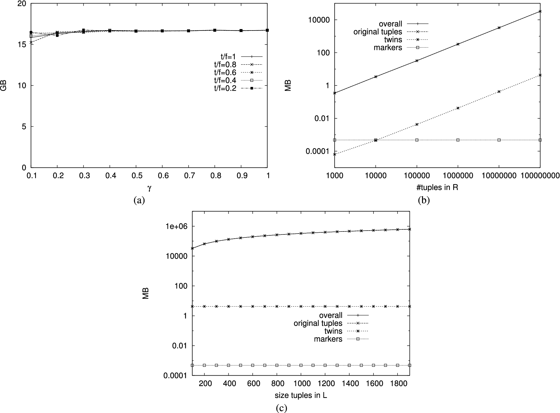
Size of extended relations with slim twins and slim markers, varying γ and the percentage of twins (a), the number of tuples in R (b), and the size of tuples in L (c).

8.3. Slim twins and slim markers

The last set of experiments was dedicated to the analysis of the use of slim twins and slim markers, completely departing from the use of salts and buckets. The experiments considered, as a reference configuration, the same base configuration illustrated in Section 8.2.

We first analyzed the scalability of slim twins and slim markers, by measuring the size (in MB) of the relations transmitted among the parties. Figure 16(a) compares the size in GB of $R^{*} + L^{*} + J^{*}$ obtained adopting a different percentage of twins, varying the parameter γ of the Zipf distribution. It is interesting to note that (differently from what happens with salts and buckets limited to the VO) the percentage of twins and parameter γ have limited impact on the size of the extended relations. Slim twins and slim markers provide high scalability, even when the frequency distribution is skewed and all the original tuples are twinned. This is further confirmed by Figs 16(b)–(c), which show that the main contribution to the size of $R^{*} + L^{*} + J^{*}$ is the size of the original tuples in R, L, and J. These figures confirm that the contribution of twins and markers is negligible and that the approach scales well when the number of tuples in the original relations and their size grow.

Fig. 17.

Ratio between the overhead obtained with slim twins and slim markers ( ${VO}_{s}$ ), and with regular twins, markers, salts and buckets ( ${VO}_{b}$ ).

To assess the advantage provided by slim twins and markers, we analyzed the ratio $\frac{| {VO}_{s} |}{| {VO}_{b} |}$ between the number of tuples in ${VO}_{s}$ and in ${VO}_{b}$ , where ${VO}_{s}$ is the set of slim twins and slim markers. Figure 17(a) compares the ratio $\frac{| {VO}_{s} |}{| {VO}_{b} |}$ for configurations adopting a different percentage of twins. We note that the advantage provided by our optimization is higher when the frequency distribution of the values of the join attribute is skewed (i.e., γ is close to 0). However, in all the considered scenarios, the size of the verification object obtained with slim twins and slim markers is a small fraction of the overhead caused by the adoption of our base protection techniques. Like for the optimization limiting salts and buckets to the VO, the advantage is higher when the percentage of twins is lower. Figure 17(b) compares the ratio $\frac{size ({VO}_{s})}{size ({VO}_{b})}$ of configurations characterized by different sizes of the tuples in L and R. Again, smaller tuples provide higher advantages.

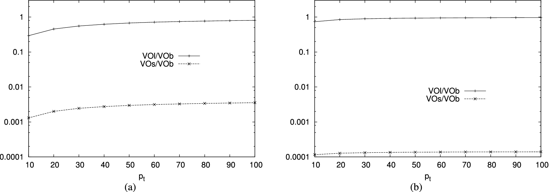
Comparing the results illustrated in Fig. 15 and in Fig. 17, we note that the adoption of slim twins and slim markers provides higher advantages than limiting salts and buckets to the verification object. To obtain a further verification of the behavior of our techniques, we performed experiments over the TPC-H database [27]. Figure 18 compares the ratio $\frac{size ({VO}_{s})}{size ({VO}_{b})}$ and the ratio $\frac{size ({VO}_{l})}{size ({VO}_{b})}$ obtained with 100 markers and varying the percentage of twins adopted by the client. Figure 18(a) illustrates the results obtained from the join between relation Orders and relation Customer, including 1,500,000 tuples of 98 bytes and 150,000 tuples of 163 bytes, respectively. Since the maximum frequency of values in relation Orders is 41, we use 7 salts and buckets with 6 tuples each. Figure 18(b) illustrates instead the results obtained from the join between relation LineItem and relation Supplier, including 6,001,215 tuples of 107 bytes and 10,000 tuples of 143 bytes, respectively. Since the maximum frequency of values in relation LineItem is 694, we use 27 salts and buckets with 26 tuples each. These results confirm the result observed on synthetic data, that is, slim tuples provide a higher benefit than limiting salts and buckets to the VO.

Fig. 18.

Ratio between the overhead obtained with slim twins and slim markers ( ${VO}_{s}$ ) and when limiting salts and buckets to the VO ( ${VO}_{l}$ ) with respect to the adoption of regular twins, markers, salts and buckets ( ${VO}_{b}$ ) over TPC-H relations.

9. Related work

Our work falls in the area of security and privacy in emerging outsourcing and cloud scenarios [3,14]. In this context, researchers have proposed solutions addressing a variety of issues, including data protection, access control, fault tolerance, data and query integrity (e.g., [2,4,6,10,15–17,24,25,34]). The solutions proposed for data integrity traditionally adopt digital signature (e.g., [13]), or watermarks inserted in the dataset to also prove data authenticity and ownership (e.g., [11]). Alternative solutions are based on auditing (e.g., [29]) or on Proof Of Retrievability (e.g., [18]) and Provable Data Possession (e.g., [1]) techniques. Current solutions addressing the problem of verifying the integrity (i.e., completeness, correctness, and freshness) of query results are instead based on the definition of a verification object returned with the query result. Different approaches differ in the definition of the verification object and/or in the kind of guarantees offered, which can be deterministic or probabilistic. For instance, some proposals are based on the definition of an authenticated data structure (e.g., Merkle hash tree or a variation of it [21,33] or of a signature-based scheme [22,23]) that allows the verification of the correctness and completeness of query results. These proposals provide deterministic guarantees, that is, they can detect integrity violations with certainty but only for queries involving the attribute(s) on which the authenticated data structure has been created. Some proposals have also addressed the problem of verifying the freshness of query results (e.g., [20,32]). The idea consists in periodically updating a timestamp included in the authenticated data structure or in periodically changing the data generated for integrity verification.

Probabilistic approaches can offer a more general control than deterministic approaches but they can detect an integrity violation only with a given probability (e.g., [7,12,26,28,30,31]). Typically, there is a trade-off between the amount of protection offered and the computational and communication overhead caused. The proposal in [26] specifically focuses on the verification of the inner product of vectors, exploiting the algebraic properties of this operation. The proposal in [30] consists in replicating a given percentage of tuples and in encrypting them with a key different from the key used for encrypting the original data. Since the replicated tuples are not recognizable as such by the server, the completeness of a query result is guaranteed by the presence of two instances of the tuples that satisfy the query and are among the tuples that have been replicated. The proposals in [12,28,31] consists in statically introducing a given number of fake tuples in the data stored at the external server. Fake tuples are generated so that some of them should be part of query results. Consequently, whenever the expected fake tuples are not retrieved in the query result, the completeness of the query result is compromised. While the solution in [31] relies on encryption to guarantee that markers cannot be recognized by the storing server, the approach in [12] operates with plaintext data thus enhancing query performance. The combined adoption of markers, twins, salts and buckets for assessing the integrity of join queries has first been proposed in [7]. This approach has been refined in [5] to operate in a distributed scenario (i.e., MapReduce) and to support the evaluation of join chains. The original proposal has also been extended to support approximate join conditions [9]. The adoption of the semi-join evaluation strategy and the idea of limiting salts and buckets to the verification object has been first proposed in [8]. This paper considerably extends our prior work by proposing a novel optimization strategy, which enables the evaluation at an external computational server also of many-to-many joins and of star joins among an arbitrary number of relations.

10. Conclusions

We proposed efficient techniques aimed at reducing the overhead caused by integrity verification techniques. We first illustrated how markers, twins, salts and buckets can be easily adapted to provide integrity guarantees when a join query is executed as a semi-join. We then proposed two strategies to limit the size of the verification object: limiting the adoption of salts and buckets to twins and markers only, and representing twins and markers through slim tuples. The security analysis showed that our optimizations only marginally affect the integrity guarantees provided by the adoption of twins and markers. However, the same guarantees can be obtained by adopting a higher percentage of twins, which have a much lower cost (as illustrated by the performance analysis). Hence, with the same overhead, the client may enjoy higher protection. We finally described how the adoption of slim twins and slim markers enables the evaluation of many-to-many joins and star joins involving more than two relations. The experimental evaluation confirmed that our solutions limit the computational and communication overhead due to the integrity checks. Our work leaves space for further investigations. An interesting extension concerns the consideration of different trust assumptions on the storage servers, which may be not fully trusted for: properly injecting twins and markers, access in plaintext the data they store, or knowing which of their tuples participate in the join result. Another possible line of investigation concerns the extension of the approach to the consideration of multiple computational and/or storage servers, and the consideration of more generic queries.

Footnotes

Acknowledgments

This work was supported in part by: the EC within the 7FP under grant agreement 312797 (ABC4EU) and within the H2020 under grant agreement 644579 (ESCUDO-CLOUD), the Italian Ministry of Research within PRIN project “GenData 2020” (2010RTFWBH). The work of Sushil Jajodia was partially supported by NSF under grant II P-1266147.

References

Ateniese ,

Di Pietro ,

Mancini and

Tsudik , Scalable and efficient provable data possession, in: Proc. of SECURECOMM, Istanbul, Turkey, 2008.

Basu ,

Vaidya ,

Kikuchi and

Dimitrakos , Privacy-preserving collaborative filtering on the cloud and practical implementation experiences, in: Proc. of IEEE Cloud, Santa Clara, CA, 2013.

Damiani ,

De Capitani di Vimercati ,

Jajodia ,

Paraboschi and

Samarati , Balancing confidentiality and efficiency in untrusted relational DBMSs, in: Proc. of CCS, Washington, DC, 2003.

De Capitani di Vimercati ,

Foresti ,

Jajodia and

Livraga , Enforcing subscription-based authorization policies in cloud scenarios, in: Proc. of DBSec, Paris, France, 2012.

De Capitani di Vimercati ,

Foresti ,

Jajodia ,

Livraga ,

Paraboschi and

Samarati , Integrity for distributed queries, in: Proc. of CNS, San Francisco, CA, 2014.

De Capitani di Vimercati ,

Foresti ,

Jajodia ,

Paraboschi and

Samarati , Encryption policies for regulating access to outsourced data, ACM TODS 35(2) (2010), 12:1–12:46.

De Capitani di Vimercati ,

Foresti ,

Jajodia ,

Paraboschi and

Samarati , Integrity for join queries in the cloud, IEEE TCC 1(2) (2013), 187–200.

De Capitani di Vimercati ,

Foresti ,

Jajodia ,

Paraboschi and

Samarati , Optimizing integrity checks for join queries in the cloud, in: Proc. of DBSec, Vienna, Austria, 2014.

De Capitani di Vimercati ,

Foresti ,

Jajodia ,

Paraboschi and

Samarati , Integrity for approximate joins on untrusted computational servers, in: Proc. of SEC, Hamburg, Germany, 2015.

10.

De Capitani di Vimercati ,

Foresti and

Samarati , Managing and accessing data in the cloud: Privacy risks and approaches, in: Proc. of CRiSIS, Cork, Ireland, 2012.

11.

Franco-Contreras ,

Coatrieux ,

Cuppens ,

Cuppens-Boulahia and

Roux , Robust lossless watermarking of relational databases based on circular histogram modulation, IEEE TIFS 9(3) (2014), 397–410.

12.

Ghazizadeh ,

Mukkamala and

Olariu , Data integrity evaluation in cloud database-as-a-service, in: Proc. of IEEE SERVICES, Santa Clara, CA, 2013.

13.

Hacigümüs ,

Iyer and

Mehrotra , Ensuring integrity of encrypted databases in database as a service model, in: Proc. of DBSec, Estes Park, CO, 2003.

14.

Hacigümüş ,

Iyer ,

Mehrotra and

Li , Executing SQL over encrypted data in the database-service-provider model, in: Proc. of SIGMOD, Madison, WI, 2002.

15.

Jhawar and

Piuri , Fault tolerance management in IaaS clouds, in: Proc. of ESTEL, Rome, Italy, 2012.

16.

Jhawar ,

Piuri and

Samarati , Supporting security requirements for resource management in cloud computing, in: Proc. of CSE, Paphos, Cyprus, 2012.

17.

Jhawar ,

Piuri and

Santambrogio , Fault tolerance management in cloud computing: A system-level perspective, IEEE Systems Journal 7(2) (2013), 288–297.

18.

Juels and

B.S.

Kaliski Jr. , PORs: Proofs of retrievability for large files, in: Proc. of ACM CCS, Alexandria, VA, 2007.

19.

Kossmann ,

Kraska and

Loesing , An evaluation of alternative architectures for transaction processing in the cloud, in: Proc. of SIGMOD, Indianapolis, IN, 2010.

20.

Li ,

Hadjieleftheriou ,

Kollios and

Reyzin , Dynamic authenticated index structures for outsourced databases, in: Proc. of SIGMOD, Chicago, IL, 2006.

21.

Li ,

Hadjieleftheriou ,

Kollios and

Reyzin , Authenticated index structures for aggregation queries, ACM TISSEC 13(4) (2010), 32:1–32:35.

22.

Mykletun ,

Narasimha and

Tsudik , Authentication and integrity in outsourced databases, ACM TOS 2(2) (2006), 107–138.

23.

Pang ,

Jain ,

Ramamritham and

Tan , Verifying completeness of relational query results in data publishing, in: Proc. of SIGMOD, Baltimore, MA, 2005.

24.

Ren ,

Wang and

Wang , Security challenges for the public cloud, IEEE Internet Computing 16(1) (2012), 69–73.

25.

Samarati and

De Capitani di Vimercati , Cloud security: Issues and concerns, in: Encyclopedia on Cloud Computing,

Murugesan and

Bojanova , eds, Wiley, New York, 2016.

26.

Sheng ,

Wen ,

Guo and

Yin , Verifying correctness of inner product of vectors in cloud computing, in: Proc. of Cloud Computing, Hangzhou, China, 2013.

27.

The transaction processing performance council (TPC) benchmark H, available at: http://www.tpc.org/tpch/.

28.

Umadevi and

Saxena , Correctness verification in outsourced databases: More reliable fake tuples approach, in: Proc. of ICISS, Kolkata, India, December, 2013.

29.

Wang ,

Chow ,

Wang ,

Ren and

Lou , Privacy-preserving public auditing for secure cloud storage, IEEE Transactions on Computers 62(2) (2013), 362–375.

30.

Wang ,

Yin ,

Perng and

P.S.

Yu , Dual encryption for query integrity assurance, in: Proc. of CIKM, Napa Valley, CA, 2008.

31.

Xie ,

Wang ,

Yin and

Meng , Integrity auditing of outsourced data, in: Proc. of VLDB, Vienna, Austria, 2007.

32.

Xie ,

Wang ,

Yin and

Meng , Providing freshness guarantees for outsourced databases, in: Proc. of EDBT, Nantes, France, 2008.

33.

Yang ,

Gao ,

Xu and

Choi , Authentication of range query results in MapReduce environments, in: Proc. of CloudDB, Glasgow, UK, 2011.

34.

Zhu ,

G.-J.

Ahn ,

Hu ,

S.S.

Yau ,

H.G.

An and

C.-J.

Hu , Dynamic audit services for outsourced storages in clouds, IEEE TSC 6(2) (2013), 227–238.