
Abstract
Packet classification is a network kernel function that has been widely investigated over the past decade. New networking paradigms, such as software-defined networking and server virtualization, have led to renewed interest in packet classification and its upgrade from classical five-field to many-field classification. With the increasing size of the rule sets and demands for higher throughput, performing many-field packet classification at wire-speed has become challenging. In this paper, we propose an approach to classification by integrating a probabilistic data structure called the Cuckoo filter for approximate membership queries into an R-tree data structure for high-speed, many-field packet classification. Experimental results show that the proposed classifier obtains high throughput of up to 1.5 M packets per second, and requires little memory to support large rule sets (up to 1 million rules).
Keywords
Introduction
Software Defined Networking is a new approach of deploying network infrastructure for high quality network services. Packet classification is SDN function that employed to group network packets into flows through Internet routers [17]. All packets that belong to the same flow are processed in a similar manner. OpenFlow is a communication protocol that allows SDN controllers to tell switches where to send packets. SDN controller is a centralized device that makes the packet-forwarding decisions. To perform high-end network services, OpenFlow protocol uses packet classification to characterize and isolate traffic in different flows for appropriate processing [12]. Packet classification is also used in other network devices, for example, load balancers use packet classification to distribute network or application traffic across a number of servers, Firewalls use packet classification to make drop packet or not decisions, and routers use packet classification to determine each packet next hop and QoS class [2].
It is possible to classify the packet several times as it passes through the network devices. Such network devices use a set of predefined rules called the rule set to classify packets into network flows depending on multiple fields of packet headers. Each rule in the rule set contains a set of fields plus priority and an action [6]. In many-field packet classification, each rule consists of more than 15 matching fields (thus the name). The action field describes the action to take when the corresponding rule matches a packet. When more than one rule matches a packet, Internet routers apply the action with the highest-priority rule. The same action is set for all incoming packets that match the same rule in a rule set [6]. The classifier matches multiple fields against thousands of rules in the rule set. The matching process is more complicated because each field may require different matching according to its type (exact, prefix, and range). With increasing demand nowadays for Internet throughput, performing such complex processes at wire-speed has become a challenging problem.
In this work, we aim to build a packet classifier that can be installed on any OpenFlow-based network device, we used an R-tree [8] integrated with a Cuckoo filter (CF) [5] to perform many-field packet classification. We choose the R-tree because it has a best-case query time of
The proposal of the CR-tree as a new data structure that can organize the rule set in a tree data structure with low memory requirements.
The use of the CR-tree for the first time in many-field packet classification.
A performance comparison against three recent many-field packet classification techniques.
The remainder of this paper is organized as follows: Section 2 describes related work, and Section 3 the concepts of the R-tree and Cuckoo filter are described. In Section 4 the proposed many-field packet classification technique is described and Section 5 evaluates the proposed system. Finally, the conclusions of this paper are provided in Section 6.
Related works
Many hardware- and software-based solutions have been proposed to improve packet classification performance. Such hardware solutions as Ternary CAM [13] and Bitmap Intersection [10] use high-speed hardware. Such devices usually are expensive, and have scalability and portability problems. Many software solutions have been proposed to address the scalability problem. In general, currently available software algorithms can be categorized into three groups. The first is the basic data structure group. Solutions in this group are simple, and require a small amount of memory. Examples include Linear Search, Hierarchical Tries, and the Hierarchical Binary Search Tree (HBST) [11,25]. Usually, these solutions are good for small rule sets; however, they do not scale well for large rule sets. The second group of software algorithms consists of heuristic methods, such as Hierarchical Intelligent Cuttings (HiCuts) [18], Recursive Flow Classification (RFC) [19], and Tuple Space Search [23]. Solutions in this group represent the rule set as a multi-dimensional search space, and use heuristics of the rule set to partition the search space into multiple, smaller partitions. Such solutions require long preprocessing times that degrade classification performance.
Our work belongs to the third group of software solutions – the geometry-based group – to problems of scalability and portability in packet classification. We focus on solutions in this group and compare them with our solution proposed here. This group contains such solutions as Grid-of-tries [24], Cross-producing, and Area-based quadtree [3]. Most of these are classical five-field packet classification techniques. Modern OpenFlow switches enable network virtualization, and the networks thus become programmable and flexible. Recently proposed solutions focus on many-field packet classification. The authors of [22] proposed a binary search on levels (BSOL) technique. They treated each rule of the rule set as a hyper-rectangle in one-dimensional (1D) address space. They then generated a binary decision tree so that each node is associated with a space. They divided the space of each node between its children. Each node in the tree has a filter list. If the filters overlap with the spaces of the corresponding nodes, then the filters of each node are inserted into the child that overlaps with its space. In case of the parent’s space overlapping with spaces of both of its children, a filter is inserted into the child nodes. Inserting the parent space into both child nodes causes memory expansion. To minimize the number of replicated rules, the authors in [4] proposed an approach to control replication, and called it binary search on levels with replication control (BSOL-RC). BSOL and BSOL-RC have the drawback of high preprocessing time when the number of the replicated filters becomes unacceptable high due to the overhead related to the decision tree. They divide the filter set into multiple subsets and generate a hash table for each tree level. This may generate a large set of hash tables and affect classification performance. The authors of [9] used a Bloom filter in a leaf-pushing area-based quad-tree to build their classifier. They used an on-chip memories to store the Bloom filters that represent their tree nodes. The authors in [21] proposed an approach to many-field packet classification using a range-tree [28] and a hash table [16] to build an efficient search algorithm. They first constructed a range tree or hash table for each field according to its type, queried their data structure independently for incoming packet’s fields, and then merged the results of a partial search to collect the final result. This approach also requires long preprocessing times and high processing latency. In this work, we integrate the Cuckoo filter [5] with a rectangular tree (R-tree) [8] data structure to propose an efficient data structure. We call the resulting data structure the Cuckoo filter-based R-tree (CR-tree).
We use the CR-tree for many-field packet classification by constructing an R-tree from the prefix fields of each rule in the rule set, hash the remaining fields of each rule in the Cuckoo filters, and integrate these filters into the corresponding nodes. The CR-tree is a balanced tree that has high query performance and low storage requirements because Cuckoo filters are integrated into its nodes.
R-tree and Cuckoo filter data structure
In this section, the general concepts of R-tree and the Cuckoo filter are presented.
R-tree
The R-tree proposed was by Guttman in 1984 [8]. It is a dynamic index structure for spatial data that was designed to organize d-dimensional information on physical objects. Entries in R-trees are represented as d-dimensional MBRs, where each MBR is represented as a node entry in the R-tree and contains pointers to all its children excluding leaf nodes, which contain pointers to objects of the database. The original R-tree of degree M was a combination of the root, internal nodes, and leaves. Let m ⩽ M/2; then, the root node can store from two to M entries unless it is a leaf. Internal nodes and leaves can store between m and M entries. Each of the root and internal nodes has the form (mbr, p), where mbr represents the minimum bounding rectangle that describes the object, and p represents a pointer to a child node. Each entry of the leaves has the form of (mbr, oid), where mbr represents the minimum bounding rectangle that describes the object, and oid is the ID of the given object. R-trees are dynamic data structures, that is, to handle insertion or deletion operations in the R-tree, global reorganization is not necessary. Figure 1 shows a set of MBRs of some geometric data. These MBRs (R4–R14) are stored at the leaf nodes, the three MBRs (R1, R2, and R3) are larger MBRs that group the leaves’ MBRs and describe them in the internal node of the R-tree. Assuming that M = 4 and m = 2, Fig. 2 shows the corresponding R-tree of the graphical representation in Fig. 1. Assume that an R-tree stores N data rectangles. Then, the maximum value of its height h is:
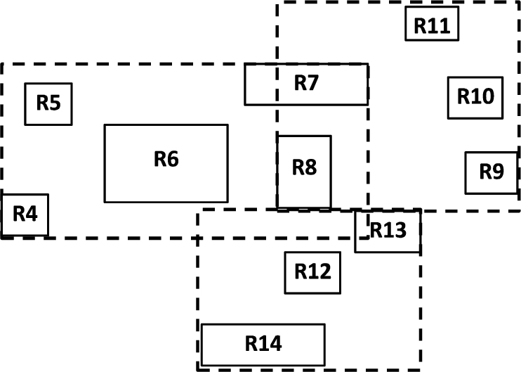
An example of a set of MBRs of geometric data.
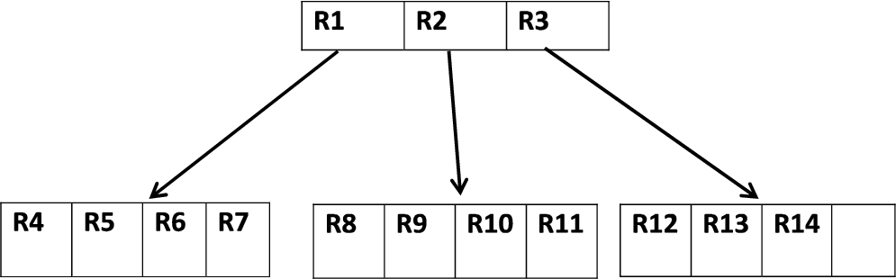
The corresponding R-tree of MBRs from Fig. 1.
The Cuckoo filter (CF) [5] is a compact, space-efficient data structure for set membership query proposed by Fan and others in 2013. The CF stores a small fingerprint for each item, and can add and remove items dynamically in
Cuckoo filter insertion
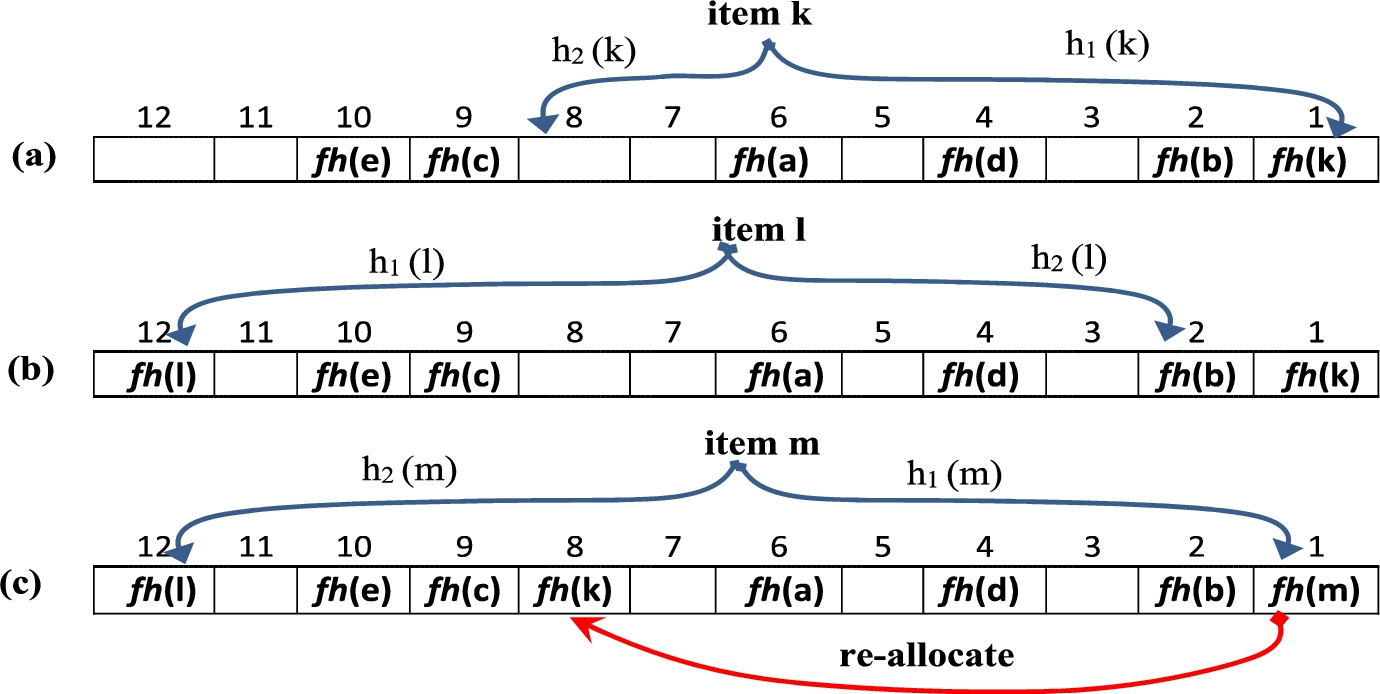
(a) Inserting “k” into bucket (1). (b) Inserting “l” into bucket (12). (c) Inserting item “m” into bucket (1).
The Cuckoo filter uses three hashing functions to add items h1( ), h2( ), and fh( ), where fh( ) creates a fingerprint for the items, and h1( ) and h2( ) are used to determine the buckets. Figure 3 depicts a Cuckoo filter twelve buckets in size, where each bucket can store one item. Initially, items a, b, c, d, and e are already inserted. Figure 3 deals with three different Cuckoo filter insertion cases. Case 1, Fig. 3(a) to add item “k”, h1(k) = 1, and h2(k) = 8. We check both buckets to determine if one is empty, in which case both buckets 1, and 8 are empty, we can add fh(k) to any one of these two buckets. We then select the first one h1(k) = 1 (bucket (1)) and insert fh(k) into it. In the second case Fig. 3(b), to add item “l”, h1(l) = 2 and h2(l) = 12. In this case, one bucket is empty (bucket (12)), and we can add fh(l) to this empty bucket. In the third case Fig. 3(c), to add item “m”, h1(m) = 1 and h2(m) = 12. In this case, both buckets are non-empty. In this case, we add “m” to one of the buckets (bucket 1), and remove an existing item from it (“k”), and re-allocate the old item into its alternative bucket (bucket 8) from case 1. The process of removing existing items and re-inserting them in alternative buckets is called the reallocation process. In some cases, reallocating an old item may also require removing another existing item, and this procedure may need to be repeated until an empty bucket is found or a maximum number of reallocation are reached (160 times in our classifier).
The Cuckoo filter has a simple query process. To query it for a given item α, we first calculate α’s fingerprint fh(α) and two related bucket indices h1(α) and h2(α), then the two buckets are read. If the fingerprint fh(α) has a match in h1(α) or h2(α) buckets, a positive result are returned; otherwise, a negative result are returned. The Cuckoo filter has advanced features to ensure that there is no false negative as long as bucket overflow never occurs for better query performance, and supports deleting items dynamically.
The proposed system architecture
The proposed packet classifier generates a rectangular tree (R-tree) from the rule set using Source IP address (SIP) and Destination IP address (DIP) fields from each rule. The classifier represents the SIPs and DIPs as MBRs in the R-tree. Following this, it hashes all remaining fields on a Cuckoo filter integrated with each MBR. The resultant tree is an R-tree that describes the rules as MBRs integrated with Cuckoo filters. Figure 4 shows the detailed block diagram of the proposed system. In the following subsections, we explain each component.
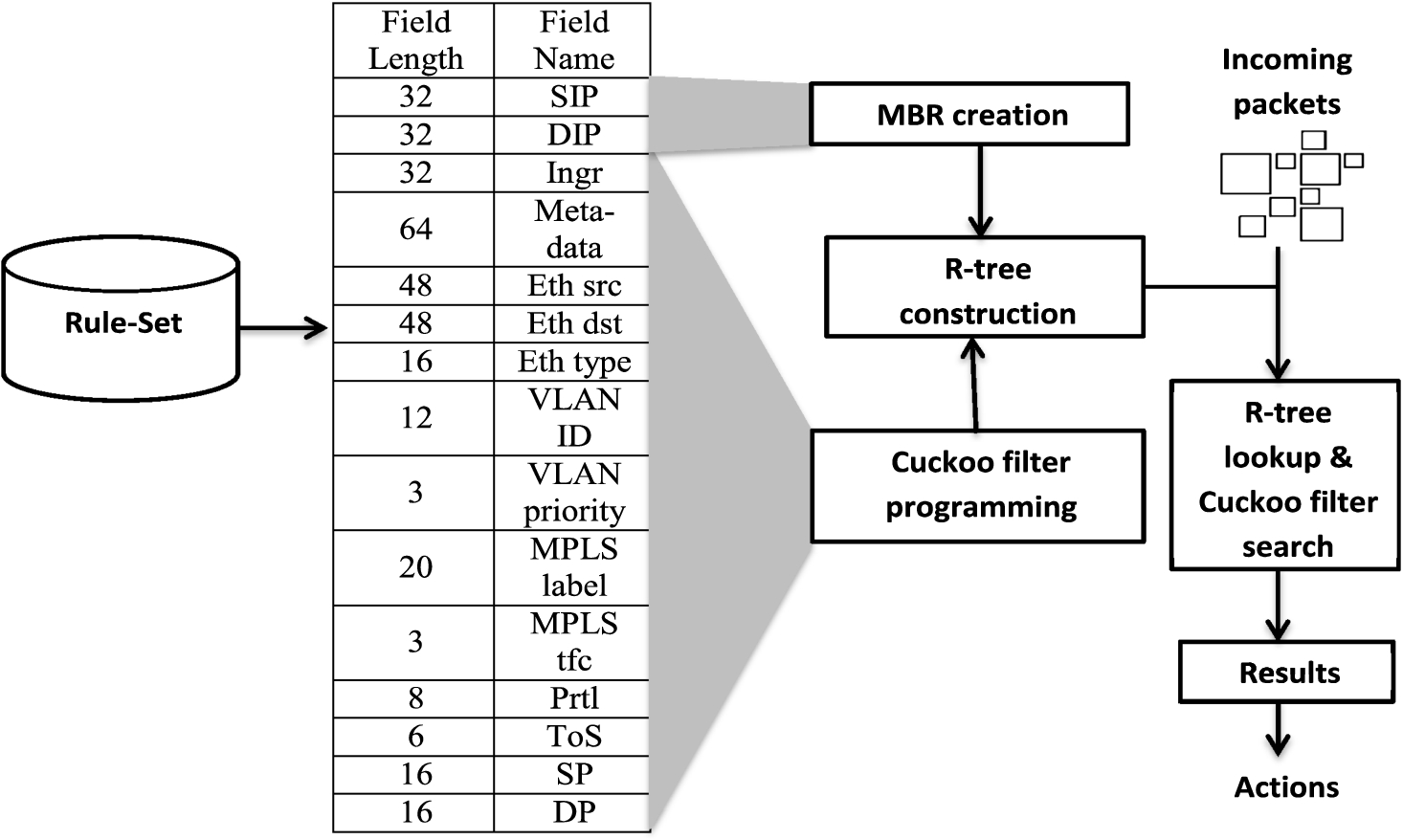
Block diagram of the proposed system.
Each rule in the rule set consists of 15 fields as shown in Fig. 4. We converted the rules into MBRs by converting their SIPs and DIPs into ranges. The minimum possible value of the prefix represents the start of the range and the maximum possible value its end. To understand the process of creation of MBR in more detail, we consider a simple set of 12 rules as depicted in Table 1. We have shown only the source/destination IP addresses necessary for creating the MBRs because each rule has two prefixes. We change these prefixes to ranges as R.Start and R.End. The two ranges belonging to the same rule represent its MBR, and can be seen as a rectangle in the geographical coordinate system. We assign a character to each rule as rule ID (RID).
A simple example of 12 rules with SIP and DIP, and prefix to range conversion
A simple example of 12 rules with SIP and DIP, and prefix to range conversion
After converting the SIP and DIP of each rule into an MBR, the process of inserting it into the R-tree begins. Initially, the empty R-tree contains only the root. To insert a new entry into the R-tree, we look for the proper location in the tree a new MBR by searching the tree from top levels to the leaves. At each level, the entry of the node whose MBR can cover the new MBR with the minimum area is selected, and a search is performed at the next level. At the leaves, if the selected node can accommodate the new MBR, it is inserted into that node. Otherwise, the old node is split by forming two new nodes (node1 and node2). We use the linear split algorithm (with linear time complexity) [14]. Two entries as seeds from the old node entries are selected so that the distance between them is the maximum among all peers, and assign these entries to the two new nodes. We define the distance between entries as the length of the virtual line connecting the centroids of their corresponding rectangles. Then, the remaining entries are assigned to the new nodes (node1 and node2) according to the one that can accommodate the entry with the minimum area. The new entries in the parent are assigned to the new nodes. The MBRs along the path from the new nodes to the root to cover the new MBR are then updated. Splitting in the upper level is performed if necessary. To show the process of insertion of the R-tree for the example in Table 1, the R-tree of degree M = 3 is built so that each internal node can store 2 ⩽ m ⩽ 3. Figure 5 shows the steps of insertion and Fig. 6 provides a graphical representation of the MBRs in the resulting R-tree.
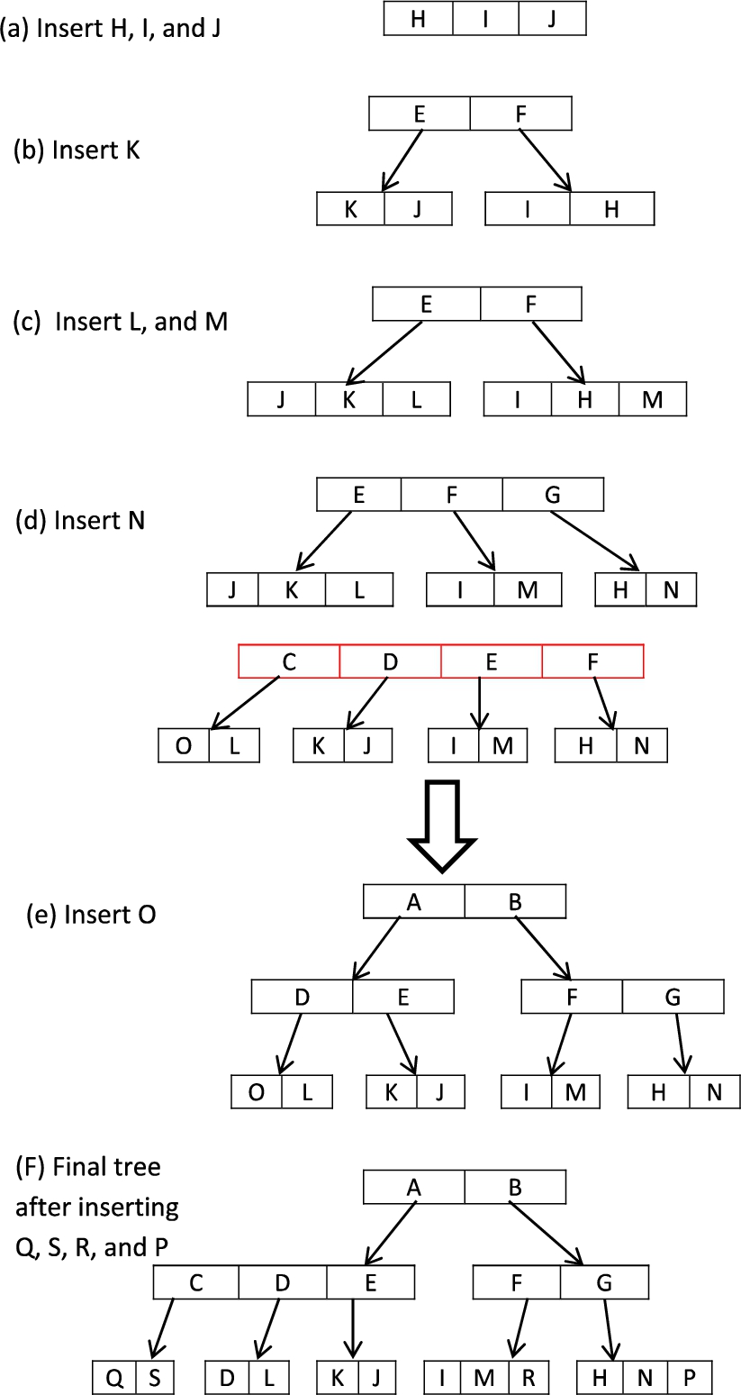
Graphical representation of MBRs from Table 1 insertion into an empty R-tree.
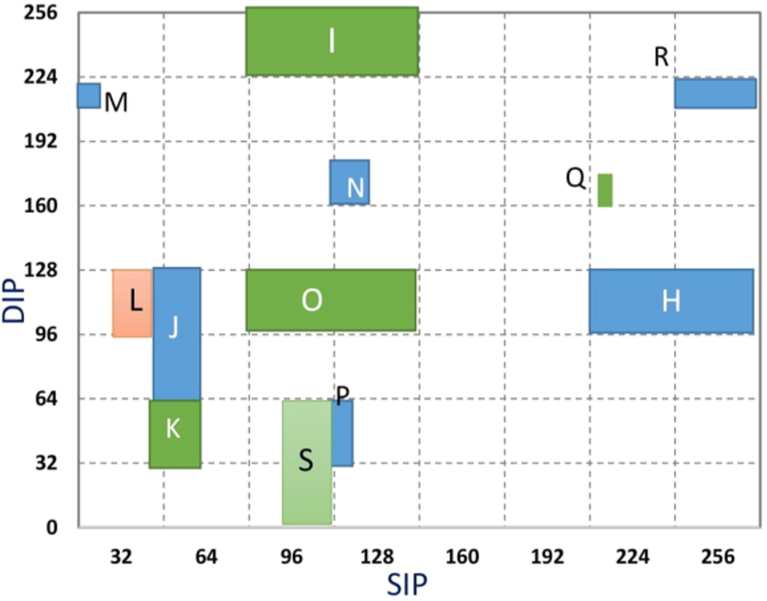
Graphical representation of the rules from Table 1.
Step (a) shows the insertion of H, I, and J into an empty root. Step (b) shows the insertion of K. In this case, the root is already full, and is this split into two new nodes to generate a new root. Then, entries E and F are assigned to the two new nodes. Step (c) shows the insertion of L and M, according to which of the node entries can cover them. Step (d) shows the insertion of N. In this case, from the perspective of the range of the SIP (96:103), N cannot be inserted into node (J–K–L) in the context of the range of DIP (160–175). N can be inserted only into the (I–H–M) branch that is already full. Splitting is thus performed. Step (e) shows the insertion of O. In this case, the selected node is already full, and splitting is performed as before. As can be observed, the parent is also full. The parent is then split. Step (f) shows the final R-tree after inserting (Q, S, R, and P).
After building the R-tree by inserting the MBRs one by one that generated using source/ destination IPs from the rule set, a Cuckoo filters are used to hash the remaining fields of each rule. The murmur hashing function [26] is modified so that all remaining fields are hashed as a fingerprint, where the hashing function generates a fixed-size binary sub-fingerprint for each field, and we use a locality-sensitive hashing function to generate locality-sensitive sub-fingerprints for the ranges of the fields [20]. Such hashing functions have the ability to hash input items so that similar items map to the same buckets with a high probability. For wildcard fields, the hashing function generates a set of zeros. The length of each field’s sub-fingerprint depends on the type and size of the field. The final fingerprint for all remaining fields is a concatenation of their sub-fingerprints in a specific order. Table 2 shows a simple example of a set of three rules tagged as H, I, and J. Each rule has seven remaining fields to be hashed as a fingerprint. It is supposed that our proposed modified murmur hashing function creates five-bit sub-fingerprints for each field (for rule sets in practice, four-bit sub-fingerprints are used for small, exact fields such as VLAN-priority, MPLS-tfc, Prtl, and ToS, eight-bit sub-fingerprints for the remaining exact fields, and 10-bit locality-sensitive sub-fingerprints for the range fields to obtain fewer collisions among the fingerprints).
A simple example of 3 rules with 7 fields
A simple example of 3 rules with 7 fields
We use a locality-sensitive hash function to generate fingerprints for the port numbers, where this function generates 10-bit fingerprints after ignoring a set of shared bits so that it takes only the shared bits from the start and the end of the range. After generating fingerprints for the shared bits, it adds four bits to the right of each fingerprint to indicate the number of the shared bits used to generate it. To indicate that the field is a wildcard field, we set 10 bits to zeros, and to indicate that the field is an exact field, we set the last four bits from the right to zero. The resulting fingerprints are
To search for a match between incoming packets and the rule sets, an MBR for each incoming packet is generated by using its SIP and DIP addresses, a query fingerprint, two bucket numbers, and its remaining fields. The R-tree is then traversed from root to leaves.
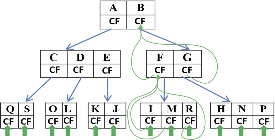
Graphical representation of integrating Cuckoo filter into the R-tree.
At each level, the node with an MBR that can cover the queried MBR with the minimum area is selected if its Cuckoo filter gives a positive result for the query fingerprint. At the leaf level, we perform a full matching check between the field of the stored rule and those of the queried packet, and report any matching rule. Following this, we select the highest-priority rule among the results. Algorithm 1 presents the R-tree query and Cuckoo filter query of the proposed system. In the CR-tree query algorithm, for each incoming packet Pkt, an MBR (Pkt.mbr) is generated, and the R-tree is traversed from root to leaves. At each level, if the given node is not a leaf node, we call the CR-treeQuery recursively for node entries that intersect the Pkt.mbr and its integrated Cuckoo filter gives a positive result. If the given node is a leaf node, we perform a full matching check between its entries and the queried packet, and add the matched rules to the answer set. We then select the highest-priority rule as a result.
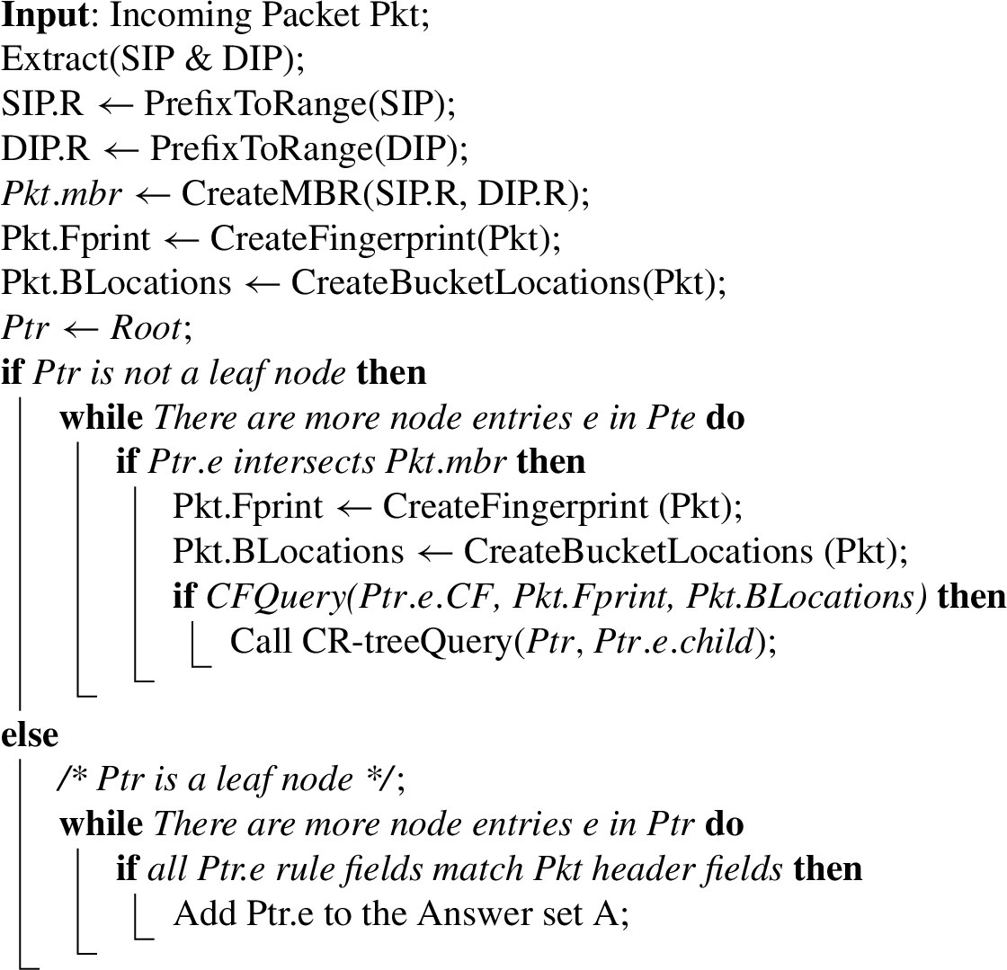
Proposed CR-tree query algorithm
For the Cuckoo filter query, the exclusive-or (X-OR) between Pkt.Fprint and the fingerprints (Ptr.e.CF) is calculated and stored in buckets locations Pkt.BLocations. If the result is zero, the queried fingerprint matches the stored one. If the result in some sub-fingerprints is non-zero, the corresponding sub-fingerprints in the stored fingerprint should be checked. If they are zero (sub-fingerprints for wildcard field), the queried fingerprint satisfies the stored one. Note that when using a Cuckoo filter, the hashing function returns insertion locations of a fixed size. The size of the Cuckoo filter increases when the level of the R-tree decreases so that the largest Cuckoo filters are at the root and smallest at the leaves. The Cuckoo filter ignores some bits from the bucket number bits according to the given level of the R-tree to fit the length of the given filter. The number of buckets remains correct because the same procedure has been used in the Cuckoo filter process.
We assume that we need to check the following packet against a Cuckoo filter containing fingerprints resulting from the rules of Table 2 in the same bucket, and that the packet also gets the same bucket: Packet = 2, 4095, AB:56, 21:8D, TCP, 91, 121. We compare it with the storied fingerprints in the Cuckoo filter. This packet matches the last fingerprint only. The last fingerprint (J) has 12 shared bits in its SP and its DP has six shared bits. Then, we convert the SP into 16 binary bits, ignore the last four bits from the right, and convert the DP into 16 binary bits and ignore the last 10 bits before sending them to the hash function. All values in the range of 80:95 are the same if we ignore the last four bits, and all values in the range 0:1024 are identical if we ignore its last 10 bits. The resulting fingerprint for the given packet is Fingerprint = 1001101010001101011111101111011011101. After applying X-or with the fingerprint for rule J without the indicating bits, the result is:
In this section, the two most commonly used metrics in the literature, query time and memory consumption, are used to analyze the proposed method. Query time (T) is the amount of time the classifier theoretically needs to classify a single packet. It has been proved in [8] that the maximum height (h) for an R-tree(
To calculate the amount of memory (M) that required to store the rule set in the proposed structure, we have assumed that L bits are required to store each MBR, C bits are required to store one item in Cuckoo filter [7].
Performance evaluation
We used a rule set with different types (access control list (ACL), firewall (FW), and IP chain (IPC)) and variable size (approximately 100 to one million rules) for each type. These rule sets were generated using the Classbench tool [1,27], and had similar characteristics to empirically used rule sets. Table 3 depicts the general properties of these rule sets. We extended these rule sets from five-field sets to 15-field rule sets by generating more static fields for each rule while the performance of proposed method does not depended on the rule’s fields specifications, and the filter deals with all fields in the same pattern, exact fields generated in any way met the purpose. Evaluations were performed on a machine with an Intel Core i7-Q720 processor, with a CPU @ 1.60 GHz 4 and 8 GB DDR3 RAM. Four evaluation metrics (classification throughput, processing latency, memory accesses, and memory requirements) were used to evaluate the proposed system.
The performance comparison against the compared many-field packet classification approaches has been conducted after re-coding and implementing these approaches on our extended rule sets and in our platform to get an equitable comparison. Further, we tested for scalability and classification accuracy. We defined the degree of the R-tree in this experiment as M = 6 and used internal Cuckoo filters with up to 1024 buckets, each with six slots, and a maximum number of relocations = 150. The size of the Bloom filter of BF-AQT was set to be identical to that of our Cuckoo filter. For BSOL-RC, we used bucket size = 4 slots that represents its optimal condition [27]. All other parameters related to the compared methods were set to the optimum condition.
The simulation rule set, and tracing data type, size, and specifications
The simulation rule set, and tracing data type, size, and specifications
We define the average classification throughput as the average number of network packets that can be classified in our proposed approach in a single second using variant type of rule sets. The proposed system can classify packets in up to 1.519 MPPS as shown in Fig. 8. The throughput of the proposed system decreased with increasing size of the rule set owing to the smaller number of memory accesses required.
Two types of R-tree have been compared against our CR-tree, so that the Cuckoo filter in our CR-tree has been replaced with a same size Bloom filter in the first type and the remaining fields have been hashed into the Bloom filters in the resulted BR-tree. And the Cuckoo filters have been removed in the second type and the remaining fields have been stored in the leaves in the resulted R-tree. As can be seen in Fig. 8, the proposed CR-tree has achieved better classification throughput in terms of different types of rule sets. Obviously, removing the Cuckoo filters from the R-tree reduces the classification throughput significantly. With Cuckoo filters integrated in the R-tree nodes, most of the unnecessary tree search (in case of successful MBR matching and failed Cuckoo filter query) has been prevented. Moreover, storing the rules in the leaves required longer query time.
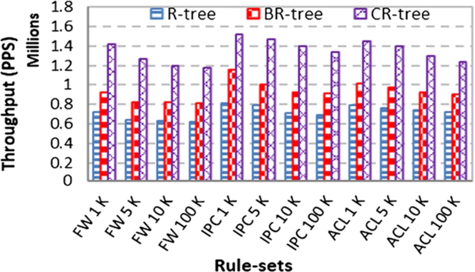
Average throughput using rule sets of different types and sizes.
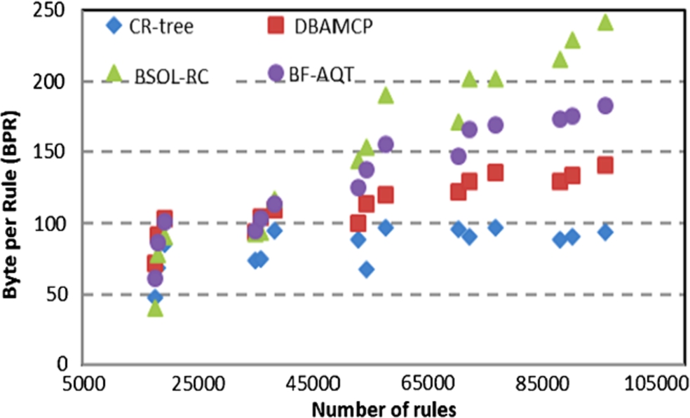
To measure memory requirements, we used bytes per rule (BpR). BpR is the number of Bytes needed to store each rule in our data structure, can be calculated by dividing the memory requirement of the entire data structure by the number of rules in the represented rule set in our data structure. The resulted BpR of the proposed approach was compared against three well-known packet classification approaches: BSOL-RC [4], BF-AQT [21], and DBAMCP [9]. All the compared approaches in Fig. 9 including the proposed approach are evaluated on the same 15-fields rule set that generated by the same tool (Classbench tool) and using the same system. Figure 9 shows the required BpR for the proposed approach, DBAMCP, BSOL-RC, and BF-AQT. The proposed approach required 50 to 106 bytes to represent each rule for rule sets of sizes (20–100) K. As a result, our data structure did not incur any exponentially increase in memory.
Moreover, the proposed approach required only 74 Byte as average to store each rule for rule sets of sizes up to 100 K rules, which means that it can support high scalability from the perspective of memory. The proposed approach outperformed the DBAMCP and BSOL-RC by more than 1.3 times. The memory requirements of the BSOL-RC and BF-AQT grew significantly with increasing size of rule set.
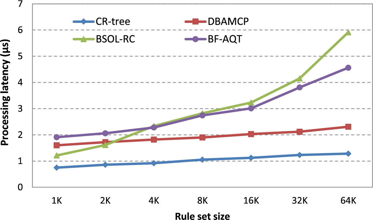
We defined processing latency as the average time required to classify a single packet measured in µs. Rule sets of sizes in range of (1–64 k) have been used to measure the processing latency of the proposed approach. The resulted processing latency has been compared against the many-field packet classifications proposed in [4] (BSOL-RC), [9] (DBAMCP), and [21] (BF-AQT). All the compared approaches in Fig. 9 including the proposed approach are related to the proposed approach as they use tree data structures as the main data structure of their classifiers integrated with secondary data structures such as Bloom filter and hash tables. In the DBAMP, range trees and hash tables have been used to perform a parallel search and the partial results have been merged from all the packet header fields to calculate the final results. The BSOL-RC has enhanced the BSOL [22] by integrating a replication control scheme. The BF-AQT uses a tree data structure combined with a Bloom filter. While the range tree in DBAMCP has a lot of internal empty nodes, the proposed approach is semi-full and balanced tree. DBAMCP also uses separated data structures to represent the remaining fields. The processing latency of the DBAMCP includes range trees query, filter query, and the process of merging of partial results. Thus, as shown in Fig. 10, our classifier outperformed the DBAMCP by more than 1.6 times in terms of latency. The authors of BSOL-RC have divided the main rule set into many sub-rule sets to fit their decision tree, that yield more that single decision tree. The BSOL-RC uses decision tree for each replicated filters set thus requires a smaller amount of memory. Therefore, as shown in Fig. 10, increasing the size of the rule sets quickly increased the latency of the BSOL-R/C. Further, the proposed approach outperformed the BSOL-RC with respect to rule sets of various sizes. The BF-AQT built a leaf-pushing area-based quadtree by assigning codewords for the SIP and DIP fields. It assigned a codeword to every SIP and DIP of the same length. For SIP and DIP with variable lengths, they determined the codewords according to shortest length. For example, a given rule with SIP and DIP = (11*, 101*), because the DIP was longer, it extended the SIP to three bits, 110* and 111*, and generated two codewords for each combined with the DIP. For the SIP and DIP that varies in length with a large number of bits, the BF-AQT produce a lot of codewords and represents these codewords in a hash table. Hence, it requires higher memory accesses and processing latency.
Memory accesses
To measure the number of memory accesses, we set the memory block size to 128 bits. The natural block size is the largest number of bits that a memory access can fetch. For each rule, up to one million packets were used as tracing data to measure the average number of memory accesses. Figure 11 depicts the average number memory access of the proposed approach.
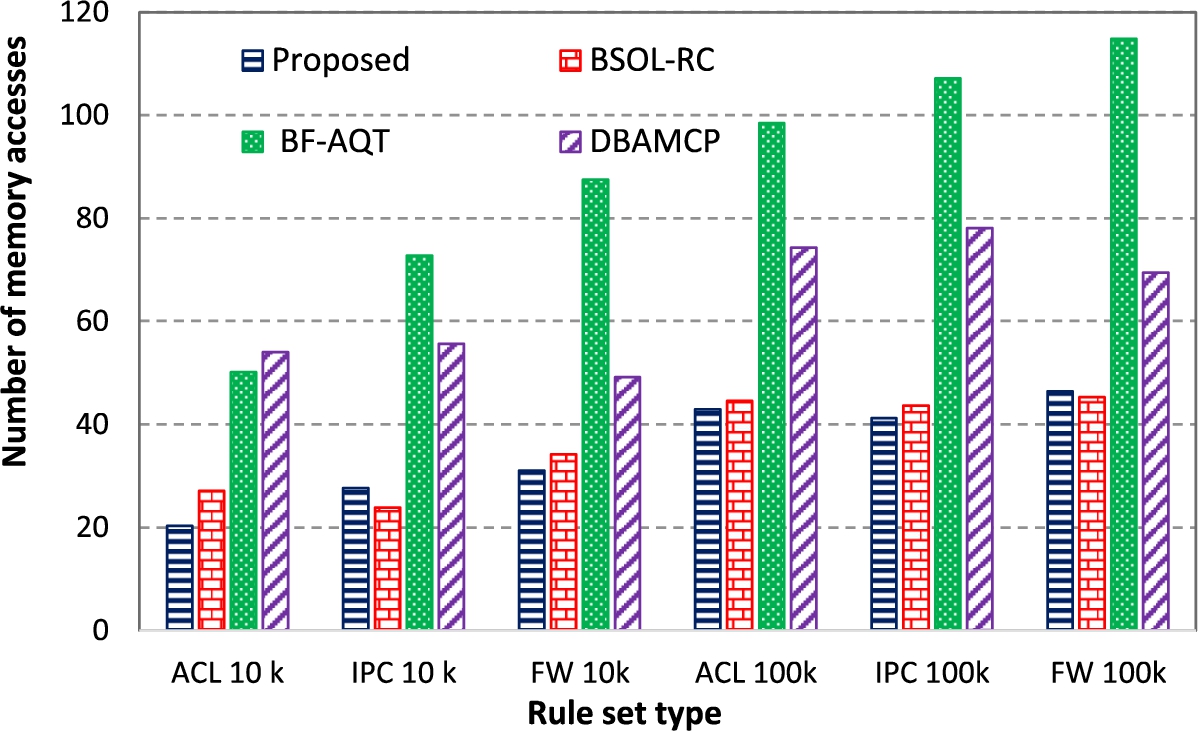
The proposed CR-tree required on average 32 memory accesses for rule sets of size up to 100 K rules. The average required memory accesses increased only when tree height increased. Thus, the average number of required memory accesses increased moderately at a very slow rate with the size of the rule sets. The proposed approach also outperformed all the compared approaches in most cases from the perspective of memory access. In some cases, the BSOL-RC was better than our approach but ours was better on average.
Typically, probabilistic data structures such as the Cuckoo filter in the proposed classifier cause some probability of false positive query result that effects the classification accuracy. While the Cuckoo filters have been used in the proposed classifier in a dynamic way, the resulted false positive probability cannot be theoretically calculated. Hence, We have calculated the false positive rate for the proposed classifier practically and compared it with the false positive rate of the case of replacing our CR-tree with BR-tree (Bloom filter integrated with R-tree) in our classifier. The results show that the proposed CR-tree had a very small false positive rate (
Comparison of false positive rates (BF = Bloom filter, CF = Cuckoo filter)
Comparison of false positive rates (BF = Bloom filter, CF = Cuckoo filter)
Tree data structures in general and R-trees in particular need relatively large storage space. We thus integrated a space-efficient data structure called the Cuckoo filter into the R-tree nodes as a query data structure for approximated membership query. In addition to its effectiveness by reducing the required storage space, Cuckoo filter helps improve the classification throughput rate because it requires a relatively short query time compared to other approximated membership query data structures. The results of simulation show that the proposed classifier achieves high classification throughput rate with low memory access, and it has high classification accuracy and better false positive rate than the same R-tree integrated with a Bloom filter instead of the Cuckoo filter.