A case based method to predict optimal k value for k-NN algorithm

Abstract

The k-nearest-neighbor classifier is a vital algorithm. In practice, the choice of k is decided by the cross-validation method. We propose a new method for neighborhood size selection based on the data set profile. The distribution of a data set and its intrinsic characteristics are the fundamental factors to the choice of k. A local complexity was computed for each example and a complexity profile was constructed by sorting these local complexity values which try to capture inner structure of a data set. After this, a feature vector was built by combing the local complexity profile and some statistic features of a data set. In addition, a history meta-data set was constructed by using the feature vector as attributes and the optimum k value of data set as the label, which was calculated by using ten cross-validation methods. A predict model was trained based on the historic meta-data set and used to predict optimum k value for a new data set. Some exclusive experiments are conducted to verify the proposed method. The results shows that the local complexity features could reflect the inner structure of a data set which could help find the optimum k for k-NN for different domains.

Keywords

k-NN classifier data sets local complexity profile optimum k

1 Introduction

The k-nearest neighbor classifier is first time introduced by Cover and Hart in 1967 [1]. It is an important benchmark classifier through [2], a data set consists of N labeled instances $\sum_{i = 1}^{N} (x_{i}, y_{i})$ . For a query vector x_q, the k-NN classifier tries to find the k nearest neighbors of x_q and incorporating majority voting method to determine the class label of x_q. Without prior knowledge, Euclidean distances are often used as distance metric. Despite its simplicity, it still yields competitive results compared with other sophisticated classifiers. Figure 1 gives an example that shows the principle of k-NN classifier and x_q will be assigned with red class.

Fig.1

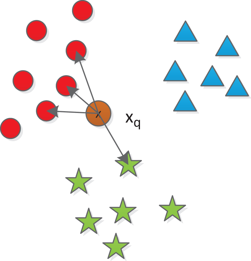
The principle of k-NN classifier.

The performance of a k-NN classifier is primarily determined by the choice of k and the distance metric used [3].

However, it has been shown when the points are not uniformly distributed; predetermining the value of k becomes difficult. Consequently, choosing the optimal k becomes almost impossible for different applications. Usually, larger values of k are less sensitive to the noise presented, and make the boundaries smoother between classes.

A number of researches have been conducted on how to choose an optimum k for k-NN algorithm, such as [4] indicates that the k should satisfy the rule k → ∞ , k/n → 0. Where n is the number of the examples in the training data set.

However, this rule can’t be used for data with a small number of examples. Peter et al. [5] and Stone [6] used cross validation method to conduct a grid search for the optimum k. However, this method needs huge computation cost and will get two or more values of k.

Although studies have been focused on this topic for a long time, the selection of k value for k-NN algorithm is still very difficult and challenging [7, 8]. For example, Lall and Sharama [9] mentioned that the suitable setting of k value should satisfy $k = \sqrt{N}$ for the datasets with a sample size larger than 100. However, such a setting has been proved to not suitable for all cases of datasets [10]. According to Bayesian method, the problem of choosing k could be classified as a model selection problem [11–14 , 26].

In addition, two key points are worth noting in some real data sets. First, a majority of the optimum k value is 1. Second, a number of data sets are not sensitive to the choice of k value. Some experiments are conducted on publicly available data sets known as UCI data sets to show the distribution of optimum k value. The accuracy of data set is calculated by using k value from 1 to $\sqrt{N}$ where N is the total number of example set in a data set. For the implementation of k-NN Weka and the ten-fold cross validation method is used. The distance measure and voting method used are mixed Euclidean distance inverse weighted voting strategy respectively. A normalization preprocess is applied to all data sets before evaluating their accuracy.

Figure 2 shows that the accuracy of data set varies with a different k value.

Fig.2

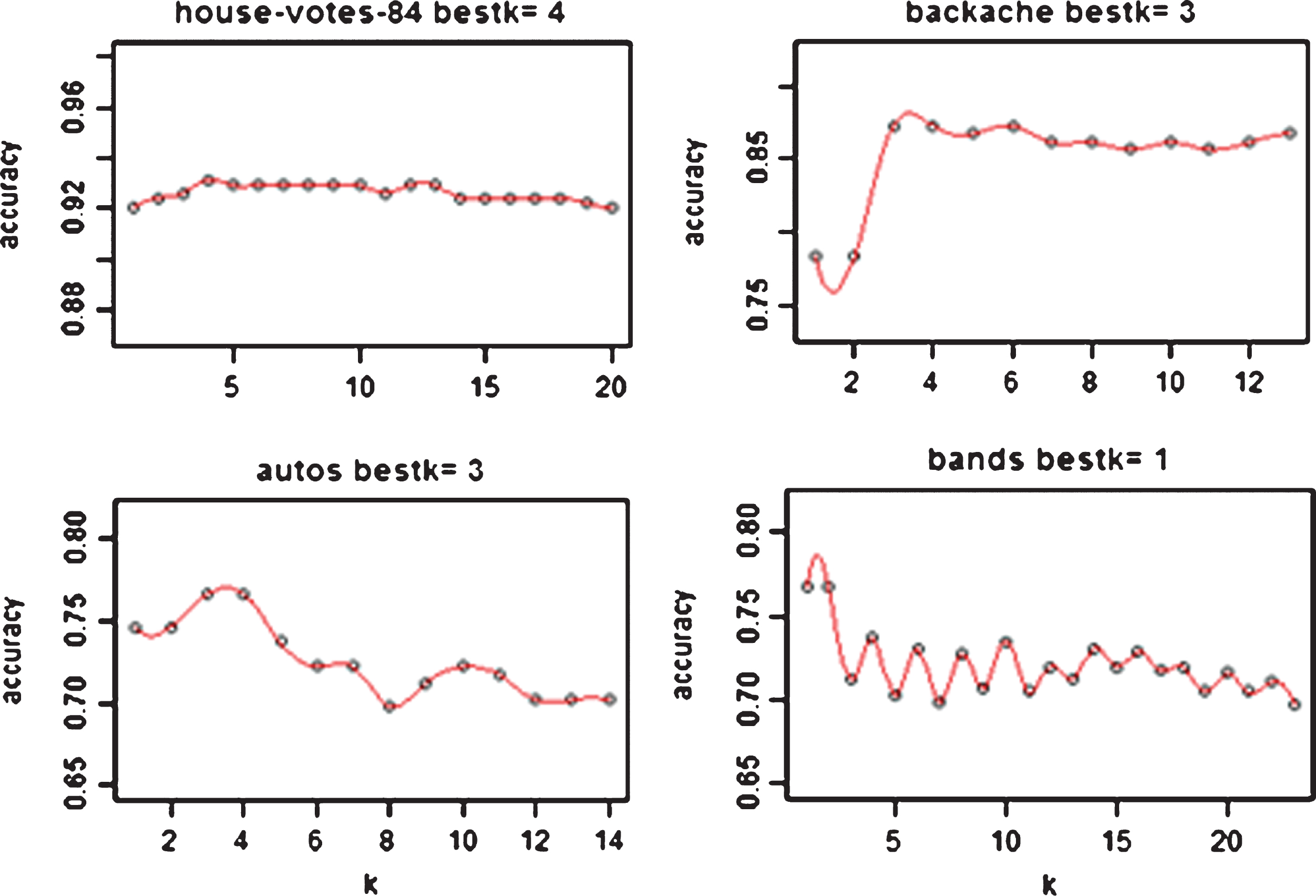
The accuracy of four UCI datasets.

The above Figures house-votes-84 is not sensitive to k value and the best performance could be achieved on a small k. On the contrary, autos, bands and backache are very sensitive to k value. But all of the four data sets achieve the best accuracy with a relatively small k value. More details about the distribution of best given in Fig. 3.

Fig.3

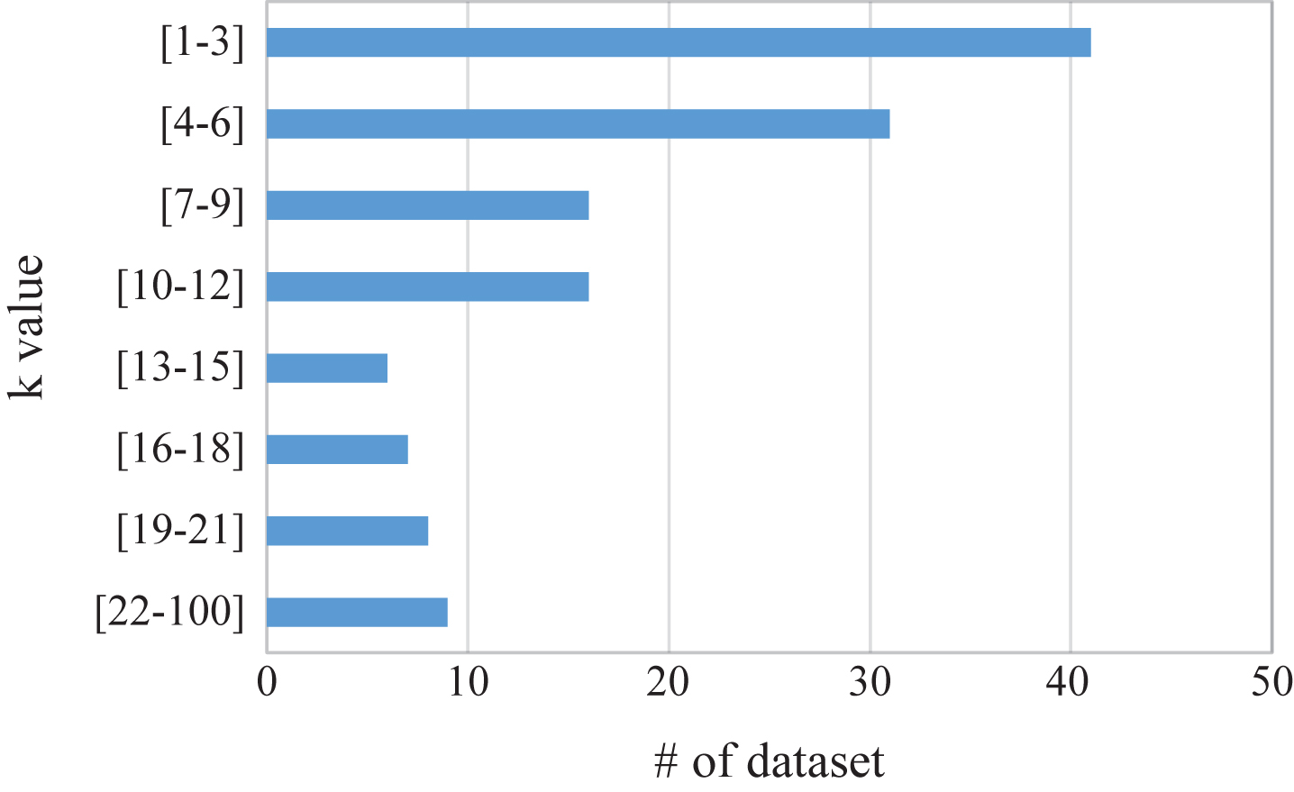
Best k value of k-NN on UCI datasets.

From the distribution of k value, it can be conclude that 1 is the most frequent best k value for many data sets. Moreover, a mall k value, usually smaller than 15, occupies a huge percentage of all the k values and the percentage is 82%. So in the process of computing the optimum k value by using grid search method, the smallest k value will be picked as optimum k when multiple k value share an equal performance.

A more recent study focus on the dataset characteristics and algorithm selection problem. In fact, classification algorithm performance is linked to data set characteristics deeply. According to Quinlan [15], “it is an important task to dig into data set characteristics and gain more knowledge of problems which could help to choose a suitable algorithm for a certain real problem”. Likewise, the study conducted by Ali and Smith [16] confirmed that, the strategy of understanding knowledge of dataset characteristics and using it to assist choosing parameters is useful.

Given these parameter selection methods may need huge computation cost and are only suitable for some special situations, such as normally distributed data sets. Simultaneously, exploring the inner structure of data set and utilizing knowledge of historic data sets are helpful to choosing optimum k for k-NN algorithm.

Based on the above analysis, we follow the meta-learning method to solve the k choose method. Firstly, we try to capture the characteristics of data set and build relationship between them and optimum k. In this paper, a feature vector as the representation of a data set is extracted based on data complexity profile and some statistical features. Additionally, a predict model is built on the historic meta-data set and is applied to predict the final optimum k value for a new data set.

The rest of the paper describes our approach and their evaluation on public domain cases. In Section 2 we review existing studies on predicting optimum k value techniques. The details computing of local complexity are presented in Section 3. Our new predicting k value technique based on complexity profile method is introduced in Section 4. Experimental results based on an amount of real datasets are reported in Section 5. Finally, we provide conclusions and recommendation for future work in Section 6.

2 Related works

In the k-NN literatures, there are several prior studies focusing on the selection of k, which recommends an optimal k for k-NN [11 –14] although cross validation is frequently used in a real data mining task.

Ghosh [11] tried to solve the multiple optimizer problems using a Bayesian method and verified the method on some benchmark data sets.

Besides, some studies considered special distribution of data set, such as Poisson or Binomial distribution. Hall and his colleagues [12] considered the choice of k under these two distributions. In addition to their work, Hand and Vinciotti [13] explored the choice of k for two-class nearest neighbor classifier when data set is severely imbalanced.

Wang et al. [14] applied a method to estimate an optimum k from the angle of statistical decision. Their method dynamically adjusts k value until a satisfactory level of confidence is reached. Holmes and Adams [17] described a Bayesian approach which integrates over the choice of k.

Wettschereck and Dietterich [18] applied a cluster algorithm to divide the input patterns into clusters. One k is assigned to each cluster which will be used to determine the size of neighborhood. Their experiments shows that local nearest neighbor methods could outperform conventional k-NN classifier on specific data sets.

Song et al. [19] work to solve the problem of the k parameter using two approaches: local information k-NN and global informative k-NN. They used a new concept named “informativeness” as a query-based distance metric. Their experiments indicate that their proposed method is less sensitive to the change of parameters than the original k-NN classifier.

Ghosh [20] used a dynamic k value according to the distribution of competing classes in the neighborhood of the observation to be classified. However, this method needs huge computing resources.

Recently, meta-leaning method was widely used to solve this problem. Reif [21] make use of meta-learning method to predict accuracy of different algorithms and achieved a good result. They built relationship between the model accuracy and data characteristics.

Ozger et al. [22] followed the meta-learning method to assign a k value for a particular dataset. In their study, 16 meta-features are extracted from each of 200 datasets. The meta-learning dataset consist of the 16 meta-features as the attributes and an optimum k value as the label. Based on the meta-training dataset, a decision table was constructed to predict the optimum k value for each new data set.

Unlike, some researcher focus on a dynamic k value for each instance instead of a global k for all the examples.

Faruk and Mehmet [23] incorporated an unsupervised method into the procedure of finding local optimum k value for each instance and termed their method 1NC. 1NC method was evaluated on 36 UCI data sets and achieved a better accuracy than 1-NN and 5-NN algorithm. However, their method has more time complexity than the unsupervised method. Moreover, an extra parameter M/L needs to be given.

Qingsheng et al. [24] incorporated a new concept named nature neighbor and found the nature neighbor number (NaN) to replace the parameter k. In their method, the nature number of each test point is flexible and can be viewed as a method of finding a local k value for each instance.

Bhattacharya et al. [25] proposed to utilize a non-parametric test point specific k estimation strategy to get a dynamic k for each data set. With this aim, they construct a hyper sphere around the test point to capture the local distribution of the surrounding training points.

Hassanat et al. [26] used an ensemble learning algorithm to compute class of a new example in the data set and achieved a good performance. The method combined results of numbers of weak k-NN classifier to determine the final result of a new example, therefore, no certain k value was needed.

3 Case-based complexity profile

Local complexity is a measure which reflects the complexity of the environment of an example. It is also a metric considering the distribution of the neighborhood of an instance. A low complexity value means the example is surrounded by other examples belonging to the same class while a high complexity value means the example is contained in an environment full of examples coming from different classes.

3.1 Complexity measure

With the aim to predict optimal k value for k-NN algorithm, some special measure which reflects the accuracy of k-NN algorithm directly is helpful [29]. Local complexity is a measure try to capture the degree of diversity of the neighborhood, which also decide the final class of the target example. The details are shown in Fig. 4.

Fig.4

The local complexity for an example with different distance. a) Composition of neighbors for c₁, b) Distribution of neighbors for c₁.

In Fig. 4, an example c₁ is in the center of all the circles and is displayed as circle symbol. We consider the case c₁ as target example, k as the number of size of neighborhoors, P_k is the ratio of neighbors belonging to same class with the c₁ in its k neighbors. The computing of P_k is shown in Equation 1. $P_{k} = \frac{Num (neighbor_same_class_c 1)}{k}$ (1)

Where the Num (neighbor _ same _ class _ c1) is the number of neighbors who share the same label with c₁ in the k neighbors and k is the number of neighbors.

It is worth noting that k is incrementally increasing from 1 to 4 and the corresponding ratio is 1, 0.5, 0.67 and 0. 5. The different ratio reflects different composition of its neighbors. The complexity value of this example is calculated by: $local_complexity = 1 - \frac{1}{K} \sum_{k = 1}^{1} P_{k}$ (2)

The complexity of c₁ is 1 - (1 + 0.5 + 0.67 + 0.5)/4 = 0.3325 and is shown in Fig. 4. We only need this complexity profile reflects its nearest neighbors and we choose k = 10 in our latercalculations.

However, there would be a number of neighbors with equal distance to the target example, when a data set contains multiple nominal attributes and distance metric used is overlapping method. As shown in Fig. 5, the local complexity for center example is computed by 1 - (0.67 * 3 +0.625 * 5 +0.583 * 4)/12 = 0.378.

Fig.5

The class of c₁ and its neighbors. a) Composition of neighbors for c₁, b) Distribution of neighbors for c₁.

The local complexity reflects the intrinsic data structure of a data set. Specifically, a high complexity means that the case is close to class boundaries which are uncertainty areas of problem space. In the boundaries, examples are often surrounded by cases with different class labels and will get a high local complexity. Similarly, the potential noisy instance will achieve a high local complexity. On the other side, a low complexity means that the case is contained in an environment in which all the examples share the same class label and the decision of a new problem could be made confidently. Moreover, cases with zero complexity value means that they are in the center of an extent of cases owning the same class label, and can be viewed as redundant instances. Furthermore, their neighbors could provide enough information to distinguish a new problem in the subspace.

3.2 Complexity profile

However, though the local complexity provides a local view of uncertainty of the problem space, the whole structure of data set is still obscure. A simple way to gain an insight of global structure of the data set is to build a profile by ranking the local complexity in ascending order. The established complexity profile allows us to visualize the overall complexity of a data set. Thus, it can be used to inform the similarity of data sets across domains. Take breast-cancer for instance, we first calculate complexity for each point in the data set and sort them to construct the complexity profile of the data set, the results are shows in Fig. 6.

Fig.6

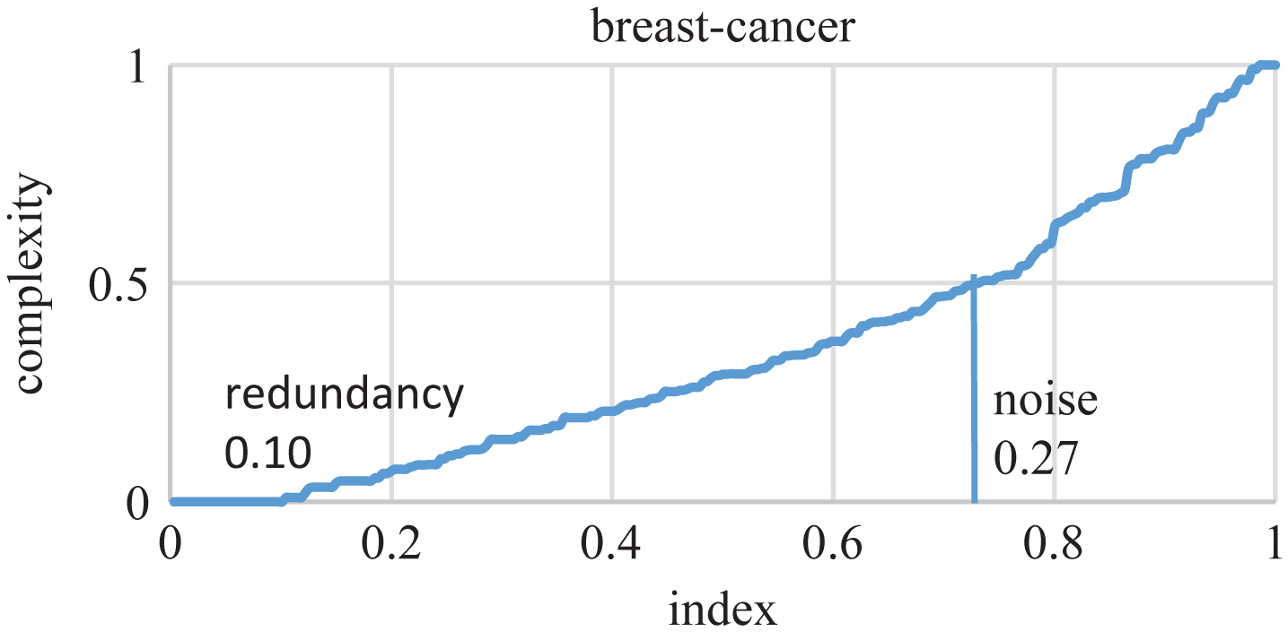
The local complexity profile for breast-cancer.

Figures 6–8 demonstrate the profile of data set which is build based on local complexity. The noise examples of a data set consist of examples with a complexity bigger than 0.5. The redundancy examples of data set consist of examples with a complexity equal to zero. For instance, the noise and redundancy of breast-cancer are 0.27 and 0.1 respectively. Comparatively, wine data set has a bigger redundancy 0.7 and a smaller noise ratio 0.04 compared to breast-cancer. More details are shown in Table 1.

Fig.7

The local complexity profile for german-credit.

Fig.8

The local complexity profile for wine.

Table 1

The noise and redundancy of data sets

Data set	Noise	Redundancy
Breast-cancer	0.27	0.1
German-credit	0.26	0.13
Wine	0.04	0.706

The data set profile can reflect the inner structure of data set to some extent. A feature vector could be extracted from the profile and will be used as representation of the data set across domains.

4 Proposed method

With the aim to predict the optimal k value for k-NN algorithm, a method of depicting data characteristics is applied. There are plenty of methods associated with building profile for a data set and can be classified into six categories: Simple info [27], statistical info [28], entropy based info [29], model based info [30], land-marking method [31], complexity based method [32]. Apart from these methods, we intend to capture inner structure of the data set [33]. The propose method builds a profile of data set by combining local complexity profile and some statistical measures. Based on these features, we could predict optimum k value for a new data set. The whole process of our proposed method is shown in Fig. 9.

Fig.9

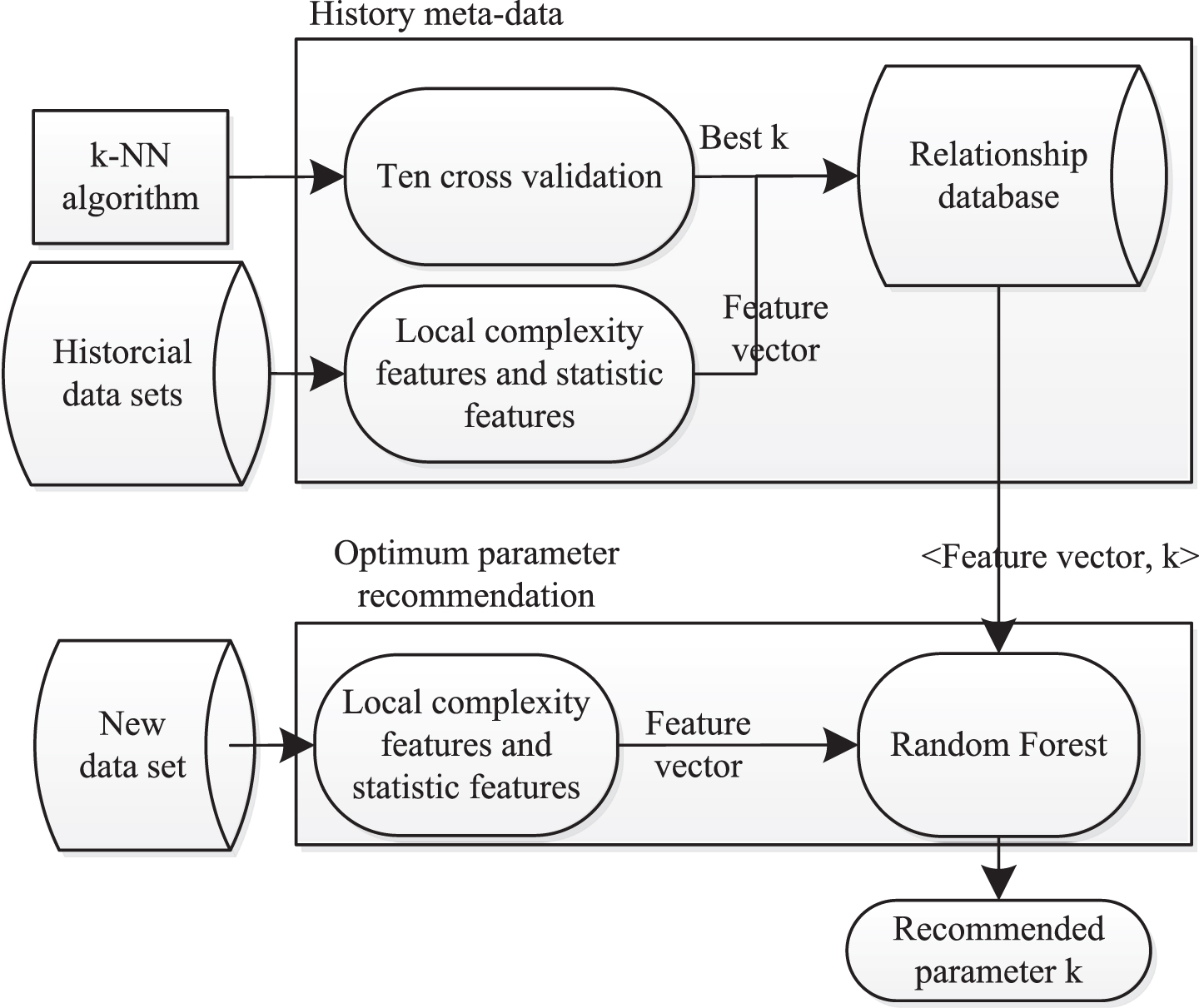
The process of predict optimum k for a data set.

The data set feature vector contains two parts. One part is the feature of data set’s complexity profile curve which was computed by using a method called local complexity. Another part consists of some statistical features about the data set. The details of these statistical features are shown in Table 2.

Table 2

The details of statistical metrics for a data set

Category	Name	Detail
Simple features	size	Number of examples
of data set	Class number	Number of class
	Feature number	Number of features
	Numeric features number	Number of numeric features
	Nominal features number	Number of nominal features
	Ratio of nominal features	Ratio of nominal features
	Ratio of numeric features	Ratio of numeric features
	Number of example of dimension	Number of example of dimension
Features of local	Mean	Mean of curve
complexity profile	Mode	Mode of curve
	Median	Median of curve
	Midrange	The mean of maximum and minimum
	Quantile	Quantile of curve
	Various	Various of curve
	CV	coefficient of variation CV
	Interquartile range	Range of third quantile second quantile
	Meandiff	The diff of mean of whole array and mean of values bigger than mean of whole
	Skewness	Skewness of curve
	kurtosis	Kurtosis of curve
	Noise	the ratio of examples with a local complexity smaller than 0.4
	Redundancy	The ratio of examples with a local complexity bigger than 0.6
	Entropy	Entropy of local complexity for all examples

The different steps of the proposed method is summarized in Table 3.

Table 3

Summary of the proposed algorithm

(1) Algorithm of building prediction model.

Input:

N_tr: number of history data set;

{D_{i}}_{i = 1}^{Ntr}

Training history data set;

k-NN: any modified k-NN algorithm;

Output:

M_history: k prediction model building by training SVM algorithm on the meta data extracted from history data set.

Procedures:

Given a number of data sets {D_i}.

Step 1: Compute feature vector of each data set F_Di which consist of local complexity profile and some statistic features.

Step 2: Compute the optimum k value under a specific k-NN algorithm for data set D_i using grid search algorithm.

Step 3: Collect feature vector F_Di and k value to construct meta-data set.

Step 4: Apply RandomForest algorithm on the meta-data to train a predict model M_history.

(2) Predicting optimum k

Input:

D_new: A new data set.

Output:

k: the predicted optimum k value for D_new.

Step 1: Compute feature vector of the new data set F_{D
_new} which consist of local complexity profile and some statistic features.

Step 2: Apply the predict model M_history to predict the optimum k value based on the feature vector of the new data set.

First of all profile of data set is constructed by using local complexity features and some statistic features as illustrated in Fig. 6 and Table 3. Besides, optimum k value for history data set is computed by using grid search method. A training meta-data set is constructed by using feature vector as attributes and using optimum k as label. A Random Forest [34] model is trained on the training data set. The feature vector of a new data set will be computed and used as input to the predict model which will recommend k value for k-NN algorithm.

4.1 Time complexities

The time complexity of the suggested method is related to two main working phases: namely the training predict model phase and the predicting k phase. The former phase could be executed offline and the time consuming depends on the selected k-NN algorithm and scale of the history data sets. The predicting k value phase is the main phase which affects the usability of the proposed method.

In the phase of predicting k value for a give new data set, a profile known as meta-feature of data set should be calculated which contains local complexity profile and some statistics. The time complexity of computing local complexity profile is O (N * log(N) * K * D), where N is the number of examples, K is the number of neighbors, D is the number of dimension of the data set. Compared with grid search method which own a time complexity of O (N * log(N) * K * D * S), where S is the size of search space, the propose method could save a lot of time.

4.2 Predict optimum k by using extracted feature vector

In our proposed method, some statistical measures are combined with the local complexity measures to construct a feature vector which is used as a representation of the data set. More details about the feature vector are given in Fig. 10.

Fig.10

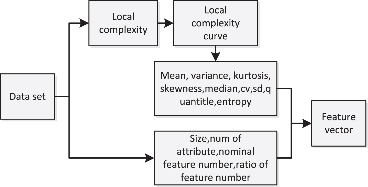
The composition of a data set feature vector.

The data set feature vector contains two parts. One part is the feature of data set’s complexity profile curve which was computed by using a method called local complexity, its details are shown in Table 2. In deed another part is some statistical information about the data set.

The details of the computed parameters are listed in Table 2 and the feature values of breast-cancer are shown in Table 4.

Table 4

Feature vector for data sets

Type	Breast-cancer	German-credit	Wine
Mean	0.347	0.32	0.062
Variance	0.288	0.274	0.162
Median	0.292	0.276	0
MidRange	0.500	0.5	0.471
CV	0.829	0.855	2.617
Quantile 25	0.106	0.078	0
Quantile 50	0.292	0.276	0
Quantile 75	0.516	0.508	0.034
Quantile 100	1	1	0.942
IQR	0.41	0.43	0.034
Meandiff	0.287	0.263	0.229
kurtosis	2.423	2.495	16.047
Skewness	0.68	0.67	3.519
Entropy	3.094	3.019	1.025
Noise	0.27	0.26	0.04
Redundancy	0.1	0.13	0.7
Size	286	1000	177
Number of attribute	10	21	14
Number of nominal feature	9	13	0
Number of numeric feature	0	7	13
Ratio of nominal feature	1	0.619	0
Ratio of numeric feature	0	0.333	0.928
Number of class	2	2	3

5 Experiment

5.1 Data sets

The data sets we used come from UCI open learning repository, 120 classification data sets are picked, containing computer application, life science, physical science, social science, e-commerce and game fields. With the aim to remove the effect of data set which is insensitive to choice of k, a number of accuracy of different k are computed. In addition, the corresponding standard deviation of accuracy is computed to evaluate whether a data set is sensitive to k or not. In the process of experiment, some data sets with big standard deviation of accuracy arechosen.

5.2 Evaluation metric

To evaluate the effectiveness of our proposed method, the difference between predicted k and optimal k are estimated by applying k-NN algorithm. Two evaluation metrics are used:

MAE (magnitude of absolute error) is the absolute difference between the two accuracies.

PRED is another commonly used evaluation metric and it is the ratio of number of data set with the MAE smaller than a threshold to the total number of data sets. Often the threshold is 4% and 5%.

Equations 3 and 4 describe the computing process of MAE and PRED respectively. $MAE = | {Accuracy}_{pre_k} - {Accuracy}_{opt_k} |$ (3) $PRED (\partial) = Num (MAE < \partial) / {Num}_{dataset}$ (4)

Where Accuracy_{pre_k} is the accuracy evaluated on the predict k, Accuracy_{opt_k} is the accuracy evaluated on optimum k value, Num (MAE < ∂) is the number of data sets with a MAE smaller than ∂ and Num_dataset is the number of test data sets.

The MAE and PRED are used to evaluate how well the predicted k could fit the optimum k. In addition, some comparisons with previous optimum k choosing method are demonstrated to show the effectiveness of our proposed method.

5.3 Results and analyze

We use RandomForest method as our predict model assumed it could overcome over fitting problem, insensitive to noise and will performs well on many data sets. Ten-fold cross validation method is used to help to evaluate the RandomForest model.

There are some optimum k choosing methods, most of them are not directly recommend an optimum k for k-NN algorithm. Instead, a local dynamic k value is used in process of their k-NN algorithm. Although a better accuracy may achieved by their methods, a huge compute resource are also needed. Some experimental results are given in Table 5.

Table 5
Details of predicted k and optimum k

Name SD of Accuracy Accuracy Accuracy Accuracy for Method Method Method Opt_k Pre_k

Accuracy for 1 for 5 for $\sqrt{N}$ predicted k [23] [25] [26]

balance-scale 0.0116 0.866 0.88 0.901 0.901 0.8579 0.86 9 10

breast-cancer 0.005 0.731 0.738 0.703 0.727 0.7049 4 11

Waveform 0.023 0.736 0.789 0.819 0.828 0.7519 0.84 65 17

Ionosphere 0.008 0.863 0.849 0.641 0.852 0.8638 0.8777 0.89 2 8

house-votes-84 0.003 0.924 0.926 0.841 0.926 0.9218 0.93 4 5

spectf-heart 0.029 0.675 0.688 0.6 0.75 0.7837 0.7394 0.79 4 4

Glass 0.015 0.701 0.72 0.631 0.72 0.6722 0.6940 0.67 4 4

Wine 0.0077 0.949 0.955 0.949 0.96 0.9746 0.96 13 3

vowel 0.0187 0.993 0.968 0.955 0.965 0.8972 0.94 1 6

pima_diabetes 0.0114 0.702 0.732 0.651 0.737 0.7337 27 16

ecoli 0.02 0.804 0.866 0.426 0.875 0.7245 0.8517 8 8

segment 0.009 0.966 0.955 0.886 0.96 0.9527 0.8633 0.96 1 4

vehicle 0.013 0.699 0.733 0.611 0.703 0.6589 0.7276 0.67 5 12

iris 0.004 0.953 0.953 0.96 0.953 0.9533 0.9494 0.96 4 3

sonar 0.042 0.865 0.856 0.654 0.856 0.8212 0.8616 0.85 1 5

letter-recognition 0.04 0.905 0.891 0.617 0.869 0.9404 0.94 1 12

liver-disorders 0.0164 0.617 0.603 0.58 0.641 0.64 15 12

Name	SD of	Accuracy	Accuracy	Accuracy	Accuracy for	Method	Method	Method	Opt_k	Pre_k
balance-scale	0.0116	0.866	0.88	0.901	0.901	0.8579		0.86	9	10
breast-cancer	0.005	0.731	0.738	0.703	0.727	0.7049			4	11
Waveform	0.023	0.736	0.789	0.819	0.828	0.7519		0.84	65	17
Ionosphere	0.008	0.863	0.849	0.641	0.852	0.8638	0.8777	0.89	2	8
house-votes-84	0.003	0.924	0.926	0.841	0.926	0.9218		0.93	4	5
spectf-heart	0.029	0.675	0.688	0.6	0.75	0.7837	0.7394	0.79	4	4
Glass	0.015	0.701	0.72	0.631	0.72	0.6722	0.6940	0.67	4	4
Wine	0.0077	0.949	0.955	0.949	0.96		0.9746	0.96	13	3
vowel	0.0187	0.993	0.968	0.955	0.965	0.8972		0.94	1	6
pima_diabetes	0.0114	0.702	0.732	0.651		0.737		0.7337	27	16
ecoli	0.02	0.804	0.866	0.426	0.875	0.7245	0.8517		8	8
segment	0.009	0.966	0.955	0.886	0.96	0.9527	0.8633	0.96	1	4
vehicle	0.013	0.699	0.733	0.611	0.703	0.6589	0.7276	0.67	5	12
iris	0.004	0.953	0.953	0.96	0.953	0.9533	0.9494	0.96	4	3
sonar	0.042	0.865	0.856	0.654	0.856	0.8212	0.8616	0.85	1	5
letter-recognition	0.04	0.905	0.891	0.617	0.869	0.9404		0.94	1	12
liver-disorders	0.0164	0.617	0.603	0.58	0.641			0.64	15	12

We use win/tie/loss to evaluate the two algorithms on multiple data sets. It can be perceived from Table 6 that our approach achieve a result of 10/0/4 corresponding to win/tie/loss compared with method in [23], 6/0/4 corresponding to win/tie/loss compared with method in [25] and 5/2/5 corresponding to win/tie/loss compared with [26]. From the statistical view, our method could achieve an equal or better result compared with [23 , 26]. However, there are very small differences between these algorithms. An explicit k value is import when some changes will be made to k-NN algorithm, such as using a different distance metric.

Table 6

The PRED (%) of the all the data sets

PRED	PRED(4)	PRED(5)
Value (%)	84.4	91.1

We also demonstrate the comparison of their accuracy based on predict k and optimum k in Fig. 11 and a statistical result in Table 6.

Fig.11

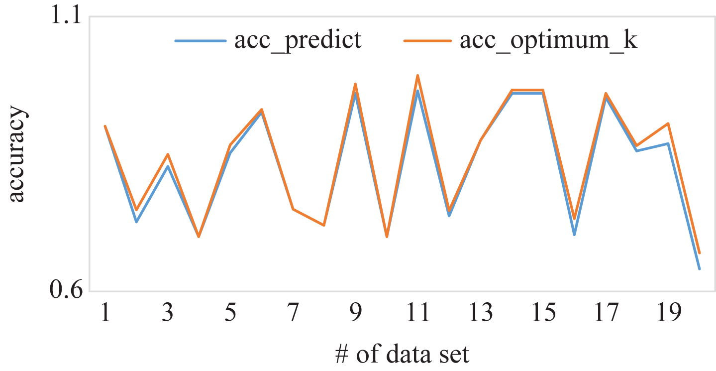
The accuracy of k-NN under predict k and optimum k.

As demonstrated in Table 6 over 84 percent of the data sets achieve a small MAE (4%). With an increasing size of history data sets, we could predict optimum k for a new data set more precisely.

Furthermore, the proposed method can compute fast, as it only needs to compute, local complexity and some dimensional info for a data set.

In the RandomForest model, we could compute the weight of all the attributes by using a method named IncNodePurity. The feature weight is shown in Fig. 12.

Fig.12

The weight of feature used in the meta-learning.

As is shown in Fig. 12, the features come from local complexity profile such as entropy, skewness, iqr, noise and kurtosis are ranked in the top seven import factors. Also, it is found that the Dimensionality and NumofSample are the most import two features in the model of predicting optimum k value.

6 Conclusion

The proposed method attempts to calculate optimal k value for k-NN algorithm based on data set’s intrinsic characteristics. Firstly, a local complexity method was used to build profile for a data set. In deed based on these profiles and dimension information of a data set, a feature vector containing mean, median, midrange, skewness and other metrics was extracted to be representation of data set. For each history data set, a feature vector and an optimum k value is computed which could be used as meta-data. Based on the meta-data of data sets, a predict model was built and used to predict k for new data set. The experimental results show effectiveness of the proposed method.

The proposed method follows the idea of first studying the data set’s own characteristics and then build relationship between them and to the classification algorithms. The accuracy of predicted optimal k value is close to optimal k value. Moreover, the proposed method could be extended to predict parameters for other algorithms easily, as it only need to compute meta-data of a data set. In addition, the calculation process implies that it only needs to compute distance of each instance without considering the type of attribute. So, it is suitable for data sets containing mixed attribute type. The future work might be focused on predicting k value for unsupervised algorithm such k-means.

References

Cover

and Hart

, Nearest neighbor pattern classification, IEEE Transactions on Information Theory13(1) (1967), 21–27.

, et al., Top 10 algorithms in data mining, Knowledge and Information Systems14(1) (2008), 1–37.

Latourrette

, Toward an explanatory similarity measure for nearest-neighbor classification, European Conference on Machine Learning. SpringerBerlin Heidelberg, 2000.

Loftsgaarden

D.O.

and Quesenberry

C.P.

, A nonparametric estimate of a multivariate density function, The Annals of Mathematical Statistics36(3) (1965), 1049–1051.

Lachenbruch

P.A.

and Ray Mickey

, Estimation of error rates in discriminant analysis, Technometrics10(1) (1968), 1–11.

Stone

, Cross-validation: A review 2, Statistics: A Journal of Theoretical and Applied Statistics9(1) (1978), 127–139.

Kang

and Cho

, Locally linear reconstruction for instance-based learning, Pattern Recognition41(11) (2008), 3507–3518.

Meesad

and Hengpraprohm

, Combination of knn-based feature selection and knn based missing-value imputation of microarray data, In 3rd International Conference on Innovative Computing Information and Control, IEEE ICICIC’08, Dalian, China, 2008, 341–344.

Lall

and Sharma

, A nearest neighbor bootstrap for resampling hydrologic time series, Water Resources Research32(3) (1996), 679–693.

10.

Liu

, et al., A new classification algorithm using mutual nearest neighbors, In Ninth International Conference on Grid and Cloud Computing, IEEE, Nanjing, China, 2010, 52–57.

11.

Ghosh

A.K.

, On optimum choice of k in nearest neighbor classification, Computational Statistics & Data Analysis50(11) (2006), 3113–3123.

12.

Hall

, Park

B.U.

and Samworth

R.J.

, Choice of neighbor order in nearest-neighbor classification, The Annals of Statistics36(5) (2008), 2135–2152.

13.

Hand

D.J.

and Vinciotti

, Choosing k for two-class nearest neighbour classifiers with unbalanced classes, Pattern Recognition Letters24(9) (2003), 1555–1562.

14.

Wang

, Neskovic

and Cooper

L.N.

, Neighborhood size selection in the k-nearest-neighbor rule using statistical confidence, Pattern Recognition39(3) (2006), 417–423.

15.

Quinlan

J.R.

, Comparing connectionist and symbolic learning methods, Computational Learning Theory and Natural Learning Systems: Constraints and Prospects, 1994, 445–456.

16.

Ali

and Smith

K.A.

, On learning algorithm selection for classification, Applied Soft Computing6(2) (2006), 119–138.

17.

Holmes

C.C.

and Adams

N.M.

, A probabilistic nearest neighbour method for statistical pattern recognition, Journal of the Royal Statistical Society: Series B (Statistical Methodology)64(2) (2002), 295–306.

18.

Wettschereck

and Dietterich

T.G.

, Locally adaptive nearest neighbor algorithms, Advances in Neural Information Processing Systems (1994), 184–184.

19.

Song

, et al., Iknn: Informative k-nearest neighbor pattern classification, European Conference on Principles of Data Mining and Knowledge Discovery, SpringerBerlin Heidelberg, 2007.

20.

Ghosh

A.K.

, On nearest neighbor classification using adaptive choice of k, Journal of Computational and Graphical Statistics16(2) (2007), 482–502.

21.

Reif

, et al., Automatic classifier selection for non-experts, Pattern Analysis and Applications17(1) (2014), 83–96.

22.

Ozger

Z.B.

and Amasyali

M.F.

, KNN parameter selection via meta learning, In 21st Signal Processing and Communications Applications Conference (SIU)North Cyprus, Turkey (2013), 1–4.

23.

Bulut

and Amasyali

M.F.

, Locally adaptive k parameter selection for nearest neighbor classifier: One nearest cluster, Pattern Analysis and Applications (2015), 1–11.

24.

Zhu

, Feng

and Huang

, Natural neighbor: A self-adaptive neighborhood method without parameter K, Pattern Recognition Letters80(1) (2016), 30–36.

25.

Bhattacharya

, Ghosh

and Chowdhury

A.S.

, Test Point Specific k Estimation for kNN Classifier, In 22nd International Conference on Pattern Recognition, Stockholm, Sweden, ICPR 2014, IEEE, Stockholm, Sweden, 2014, 1478–1483.

26.

Hassanat

A.B.

, et al., Solving the problem of the K parameter in the kNN classifier using an ensemble learning approach. arXiv preprint arXiv: 1409.0919, 2014.

27.

Engels

and Theusinger

, Using a data metric for preprocessing advice for data mining applications, ECAI (1998), 430–434.

28.

Sohn

S.Y.

, Meta analysis of classification algorithms for pattern recognition, IEEE Transactions on Pattern Analysis and Machine Intelligence21(11) (1999), 1137–1144.

29.

Segrera

, Pinho

and Moreno

M.N.

, Information-theoretic measures for meta-learning. International Workshop on Hybrid Artificial Intelligence Systems, SpringerBerlin Heidelberg, 2008.

30.

Peng

, et al., Improved dataset characterisation for meta-learning. International Conference on Discovery Science, SpringerBerlin Heidelberg, 2002.

31.

Bernhard

, Hilan

and Christophe

G.-C.

, Meta-Learning by Landmarking Various Learning Algorithms, In Seventeenth International Conference on Machine Learning, San Francisco, USA, 2000, 743–750.

32.

Cano

, Analysis of data complexity measures for classification, Expert Systems with Applications40(12) (2013), 4820–4831.

33.

Massie

, Craw

and Wiratunga

, Complexity profiling for informed case-base editing, European Conference on Case-Based Reasoning, Springer, Berlin Heidelberg, 2006.

34.

Breiman

, Machine Learning, Random Forests, 2001.