Continuous-time path planning for multi-agents with fuzzy reinforcement learning

Abstract

There are a lot of applications of multi-agent systems, such as robot navigation, distributed control, data mining, etc. Reinforcement learning (RL) is a popular method used in multi agent path planning. RL algorithm needs an accurate representation of a small and discrete space. In order to plan multi agents in continuous time, this paper approximate the Q-values with the fuzzy logic, such that the modified RL can work in continuous state space. The fuzzy reinforcement learning proposed in this paper uses fuzzy Q-iteration algorithm and a modified Wolf-PH algorithm. The convergence and existence of the algorithm are proven. The continuous time planning algorithm is applied to a cooperative task of two mobile Khepera robots. The experimental results show the effectiveness of the new path planning method for the multi agents in continuous time.

Keywords

Fuzzy reinforcement learning multi agents path planning

1 Introduction

Multi-agent systems are composed of multiple interacting intelligent agents, which can be used to solve problems such as robotics team, distributed control, resource management, collaborative decision, and data mining [1]. A multi-agent system includes several intelligent agents in an environment. Each agent has its independent behavior and should coordinate with others [2]. An important advantage of using the multi-agent system is modeling the cooperation of real-life situations. Multi-agent systems could emerge as the most natural way of looking at a system, or provide an alternative perspective on centralized systems. They include several intelligent agents in an environment, and each agent perceives the environment through sensors and actuators. At the same time, the multi-agent system can also learn new behaviors in order to adapt to the new task and objectives in the environment [3].

The reinforcement learning is one of the most popular method for multi-agent planning. The learning object is to maximize a reward function defined by the environment, such that the agents can interact with the environment and modify the environment in a good manner [4]. At each learning stage, the agent detects the environment by taking actions. For the traffic situation, it gives a new state [5]. The quality of each transition is evaluated by another reward function. In order to give the correct actions to agents, feedback RL can be used [6], which uses less informative than the supervised learning method [7]. The agents are not told what actions should be taken. They only know what actions are most rewarding.

Since RL requires accurate representations of state-action values in the environment and the policies must be in some lookup tables, the solutions are untreatable One of the challenges of the reinforcement learning for multi agents path planning in continuous-time is dimension problem [8]. The states in continuos-time and spaces have to be divided into many cells, such that the discrete-time RL can be applied. The accuracy of this RL is the dimension of one cell. In order to improve the leaning accuracy, the cell number has to be increased. However, for large space problem, the discrete-time RL cannot work well.

Most multi agents path planning approaches have to reduce the working space, or discretize the space into low dimension. However, in the real life applications the state variables have many possible values and even are continuous. RL should be combined with other methods, or be modified. [10] uses function approximation for the discrete states to reduce computation space. [11] applies vector quantization for continuos states. [12] uses normalized Gaussian network to modify Q-learning. [13] uses prediction method for heterogeneous agents. [9] applies neural networks to approximate the unknown space. The above methods are not real continuos-time path planning, because they only divide the working space into small spaces.

In order to plan the multi agents path in continuos-time, the reinforcement learning is modified in this paper. We use fuzzy quantization for the state space of the multi agents. The well known WoLF-PHC algorithm [14] is combined with fuzzy logic, such that the Q-function of the agents are partitioned through a fuzzy state space. The path planning algorithm uses fuzzy Q-iteration model to achieve the sub-optimal policy for the agents. The feasibility of the proposed method is shown with two mobile robots to finish a cooperative job.

Fuzzy reinforcement learning has been applied in the single-agent navigation [15]. From the best of our knowledge, this is the first paper on continuous-time path planning of multi-agent systems. The key technique of this paper is we use fuzzy logic to modify the classical RL to overcome the dimension problem.

2 Continuos-time path planning with fuzzy reinforcement learning

For multi agent path planning problem, the action set and given tasks are solved in a determined environment. This problem can be modeled as a stochastic game, such as a Markov decision process. The actions at any time consist of each individual agent actions. The multi-agent reinforcement learning process is a generalization of the Markov decision process, called the stochastic game [16].

Definition 1. The deterministic stochastic game G is a tuple of $G = (X, U_{1}, U_{2}, . . ., U_{n}, f, ρ_{1}, ρ_{2}, . . ., ρ_{n})$ where n is the number of the agents in the environment, X is the finite set of environment states, U_i (i = 1 ⋯ n) are the finite sets of actions available to each agent.

Providing the joint action set U = U₁ × U₂ × . . . × U_n, the state transition probability function is f : X × U → X, and the reward functions ρ_i : X × U → R. As a result of the joint action of all the agents $u_{k} = {[u_{1, k}^{T}, u_{2, k}^{T}, . . ., u_{n, k}^{T}]}^{T},$ u_k ∈ U.

In discrete time, when the joint action u_k is applied to the state x_k, the new state is $x_{k + 1} = f (x_{k}, u_{k})$

We define scalar reward for each agent as $r_{i, k + 1} = ρ (x_{k}, u_{k})$ it evaluates the effect of the action u_k .

The actions are chosen according their own policy $h_{i} : X \times U_{i} \to [0, 1]$ where all actions U_i are together the joint policy h .

In continuos-time, the above equations are $\begin{matrix} \frac{d}{dt} x_{t} = f (x_{t}, u_{t}) \\ r_{t, i} = ρ (x_{t}, u_{t}), h_{i} : X \times U_{i} \to [0, 1] \end{matrix}$

Since the rewards r_t,i of the agents depend of the joint action, their returns depend on the joint policy $R_{i}^{h} (x) = \int_{0}^{\infty} γ^{k} r_{t, i} dt$ so the Q-function of each agent relies on the joint action and the joint policy, $Q_{i}^{h} = X \times U \to R$ where $Q_{i}^{h} (x, u) = E [\int_{0}^{\infty} γ^{k} r_{t, i} dt ∣ x_{0} = x, u_{0} = u, h] .$

Each agent may have its own goal. The multi agent path planning is a full cooperation problem. So the reward for any state is the same for all agents, i.e., ρ₁ = ρ₂ = . . . = ρ_n. So the returns for all the agents are also the same, $R_{1}^{h} = R_{2}^{h} = . . . = R_{n}^{h} .$ We let all agents have the same goals, which are maximize the common long term performance (return).

Determining an optimal joint policy h^∗ in multi agent systems is an equilibrium selection problem [17]. Finding the equilibria in multi agents systems is a difficult problem. We assume all agents knows the structure of the game in the form of transition function f, and the deterministic dynamics and the reward function ρ_i. In this way, the equilibria searching becomes more tractable.

We define the best response of agent i to the opponent strategies σ_i with the maximum reward $\begin{matrix} E {r_{i} | σ_{1}, . . ., σ_{i}, . . ., σ_{n}} \\ \leq E {r_{i} | σ_{1}, . . σ_{i}^{*}, . . ., σ_{n}} \forall σ_{i} \end{matrix}$ as a Nash equilibrium. Any static game has at least one Nash equilibrium. Here each individual strategy $σ_{i}^{*}$ is a best response to the others [18, 19].

For a fully cooperative stochastic game, the learning goal is to maximize the common discounted return. The objective can be accomplished by learning the optimal joint-action values Q^∗ through value iteration by using a greedy policy [20], $Q (x_{t}, u_{t}) = ρ (x_{t}, u_{t}) + γ max_{j} Q (f (x_{t}, u_{t}), u_{j})$

The agents use the greedy policies applied to Q^∗ to maximize the common return $h_{i}^{*} (x) = arg max_{u_{i}} max_{u_{1}, u_{2}, . ., u_{n}} Q^{*} (x, u)$

The multiple joint actions of some states can be optimal. In the lack of coordination mechanism, different agents could break ties among multiple optimal joint actions in different way.

2.1 Q-iteration

We define the Q-function as Q . In the deterministic case, the Q-iteration mapping could be define by $H (q) (x, u) = ρ (x, u) + γ max_{j} Q (f (x, u), u_{j})$

The optimal Q-function Q^∗ satisfies the Bellman optimally equation [21] $Q^{*} = H (Q^{*})$

Here Q^∗ is a fixed point of H. We can start from an arbitrary Q_o and update Q in each iteration l by $Q_{l + 1} = H (Q_{l})$ (1)

H is a contraction with factor α < 1 in the infinity norm [22]. For any pair of Q-function Q₁ and Q₂, $‖ H (Q_{1}) - H (Q_{2)} ‖ \leq α ‖ Q_{1} - Q_{2} ‖$

H has a unique fixed point.

Q^∗ is a fixed point of H: Q^∗ = H (Q^∗), and Q-iteration converges to Q^∗ as l → ∞ . A optimal policy $h_{i}^{*} (x)$ can be calculated from Q^∗ using (1), in order to perform the former iteration we need a model of the task in the shape of the transition function f and reward function ρ_i .

The Q-iteration needs to save and update distinct Q-values for each state-action pair. It can only deal with finite set of state and actions, such as discrete sets [23, 24].

When the state space is continuous, the Q-function has to be in an approximated form, because an exact representation of the Q-function could be impractical or intractable [25].

2.2 Fuzzy Q-iteration

We use a vector φ ∈ Rⁿ to parameterize the Q-function. The approximator φ is based on a fuzzy partition of the continuos state space, where the action space is assumed to be discrete. There are N fuzzy sets in the fuzzy partition. The membership function is $μ_{d} (x) = X \to [0, 1] d = 1, 2, . ., N$ where μ_d (x) describes the degree of the state x to the fuzzy set d .

This membership function can be regarded as a basis function or a feature [26]. The membership function may have linguistic meaning if a prior knowledge about the Q-function is available. It is not necessary in the presented method. The number of membership functions increase with the dimensionality of the state space and the number of the agents.

Triangular functions [27] are used as the fuzzy partition in this paper. For every d exist a unique x_d (the core of the membership function), such that μ_d (x_d) > μ_d (x) ∀x ≠ x_d . Since all the others membership functions take zero values in x_d, we assume that μ_d (x_d) = 1. We have N_r triangular membership functions for each state variable x_r, r = 1, 2, . ., R, dim(X) = R .

We assume that the action space is discretized for all agents. They have the same number of actions available, $U_{i} = {u_{i j} | i = 1, 2, .., n j = 1, 2, .. M}$

There z = nNM elements stored in the fuzzy approximator φ . The membership function-action pair (μ_d, u_ij) for each agent corresponds the parameter vector φ_d,i,j. We construct a nN × M matrix for the elements of the approximator. The first column with the N elements is for the first agent. So the indexes of the parameter approximator φ_[i,d,j] means d - th membership functions for j - th action for i - th agent.

The Q-function can be also approximated by multiple-input multiple-output fuzzy rules. The state x is the input of the fuzzy rules. It produces M outputs for each agent, which correspond Q-values of each action. For each agent u_ij|i = 1, 2, . ., n j = 1, 2, . . M .

The fuzzy rules can be regarded as a zero-order Takagi-Sugeno rule [28, 29] $if x is μ (x_{d}) then q_{[i, 1]} = φ_{[i, d, 1]}; . .; q_{[i, M]} = φ_{[i, d, M]}$ (2)

The approximate Q-value is calculated by a weighted sum of the parameters φ_i,d,j $\tilde{Q} (x, u) = \sum_{i = 1}^{n} \sum_{d = 1}^{N} μ_{d} (x) φ_{[i, d, j]}$ (3)

It is a linearly parameterized approximation [30]. This approximator can be denoted by an approximator mapping $F = R^{z} \to Q$ where R^z is the parameter space, Q is the space of Q-function, the parameter φ represents the approximation of the Q-function, $\tilde{Q} (x, u) = [F (φ)] (x, u)$ (4)

Thus we do not need to store great amount of Q-values for every pair (x, u). Only z parameters in φ are needed. The mapping approximator F only represents a subset of Q [31].

In order to analyze the Q-function, φ is parameterized into a linear function. It is the same as the reinforcement learning, where the approximation F is also linear [32]. So the normalized membership functions can be seen as state-dependent basis functions.

(4) provides an approximate of Q-function. The approximate $\tilde{Q}$ is supplied as an input to theQ-iteration mapping H, ${\bar{Q}}_{l + 1} (x, u) = (H \circ F) (φ_{l}) (x, u)$ (5)

$\bar{Q}$ is not able to be stored in an explicit way [33]. Alternatively it is represented in an approximate form, using a new parameter vector φ_l+1 . This new parameter vector is obtained by a projection mapping P : Q → R^z, $φ_{l + 1} (x, u) = P ({\bar{Q}}_{l + 1}) (x, u)$ (6) which makes $\tilde{Q} (x, u) = [F (φ)] (x, u)$ as near as $\bar{Q} (x, u)$ [34]. In the sense of least square regression

$\begin{matrix} P (Q) = φ \\ φ \in arg min_{φ} [\sum_{λ}^{s} (Q (x_{λ}, u_{λ}) - F (φ) (x_{λ}, u_{λ}))] \end{matrix}$ (7) where the state samples (x, u) are used.

Because of triangular membership function and linear parameterized approximation, (7) is a convex quadratic optimization problem [35]. (7) is reduced to $φ_{[i, d, j]} = P (Q)_{[i, d, j]} = Q (x, u)$ (8)

The approximate fuzzy Q-iteration starts with an arbitrary parameter vector φ . This vector in each iteration uses the mapping $φ_{l + 1} = (P \circ H \circ F) (φ_{l})$ (9)

It stops when the difference between two consecutive parameters vector φ is greater than threshold ξ, $‖ φ_{l + 1} - φ_{l} ‖ \leq ξ$ (10)

A greedy policy can be obtained to control the system from φ^∗ (which is the parameter vector derived when l→ ∞). An action is calculated by interpolation between the best local actions for every membership function core x_d $h_{i}^{*} (x) = \sum_{d = 1}^{N} φ_{i, d} (x) u_{j_{id}^{*}}$ (11) where $j_{i, d}^{*} \in arg max F (φ^{*}) (x, u) .$

2.3 Path planning with fuzzy reinforcement learning

In order to implement the update (9), we propose a modified WolF-PHC algorithm [14]. The fuzzy Q-iteration is applied to plan multi-agent path in continuous state space.

The algorithm starts with an arbitrary φ (it can be φ = 0) until a threshold ξ is reached after several iterations. We assume the dynamics f, the reward function ρ, and the discount factor γ are known. The algorithm is as follows:

Let α ∈ (0, 1], the learning rate δ_l > δ_w ∈ (0, 1] s, initialize $ϕ (x, u) = 0, π (x, u) = \frac{1}{| U_{i} |}$ (12) where π (x, u) is the probability of chosen action u in the state x, $| U_{i} |$ is the cardinality of the set U .

Repeat

For state x, we select action u according to mixed strategy π (x) with suitable exploration. At each step a random action with probability ɛ ∈ (0, 1) is used.

Applying fuzzy Q-iteration, for Membership functions μ_dd = 1, . ., N and discrete actions U_j j = 1, . . ., M, the threshold ξ > 0

$\begin{matrix} φ_{[i, d, j]} = ρ (x, u) + γ max_{j^{'}} \\ \sum_{i = 1}^{n} \sum_{d^{'} = 1}^{N} μ_{d^{'}} (f (x, u)) φ_{[i, d^{'}, j^{'}]} \end{matrix}$ (13)

Until $‖ φ_{l + 1} - φ_{l} ‖ \leq ξ$

Update the average $\bar{π}$

$\begin{matrix} C (x) = C (x) + 1 \\ \bar{π} (x, u^{'}) = \frac{1}{C (x)} (π (x, u^{'}) - \bar{π} (x, u^{'})) \end{matrix}$ (14) where∀u′ ∈ U_i,

Move π to the optimal policy with respect to Q-table $π (x, u) = π (x, u) + Δ_{xu}$ (15) $\begin{matrix} Δ_{xu} = - δ_{xu} if u \neq arg max_{u^{'}} φ (x, u^{'}) \\ Δ_{xu} = \sum_{u^{'} \neq u} δ_{{xu}^{'}} otherwise \end{matrix}$ (16) with $δ_{x u} = \min (π (x, u), \frac{δ}{| U_{i} | - 1})$ and $\begin{array}{l} δ = δ_{w} if \sum_{u^{'}} π (x, u^{'}) ϕ (x, u^{'}) > \bar{π} (x, u^{'}) ϕ (x, u^{'}) \\ δ = δ_{l} otherwise \end{array}$ (17)

Output: $φ^{*} = φ_{l + 1}$

A greedy policy is obtained to control the system by $h_{i}^{*} (x) = \sum_{d = 1}^{N} φ_{i, d} (x) u_{j_{id}^{*}}$ (18) where $j_{i, d}^{*} \in arg max F (φ^{*}) (x, u),$ $j_{i, d}^{*}$ corresponds to a locally optimal action for the core x_d for the agent i.

(13) corresponds to $H (\tilde{Q} (x, u)),$ $\tilde{Q} (x, u) = F (φ) .$ According to (8), φ_[i,d,j] = P (Q) _[i,d,j] = Q (x, u) . So the fuzzy Q-iteration (9) is updated.

Theorem 1. The fuzzy Q-iteration (9) with the above algorithm converges to a fixed vector φ^∗.

Proof 1. Since the mapping approach given by F, $[F (φ)] (x, u) = \sum_{i = 1}^{n} \sum_{d = 1}^{N} μ_{d} (x) φ_{[i, d, j]}$ the convergence of the approximate Q-iteration is guaranteed to ensure that the compound P ∘ H ∘ F mapping is a contraction in the infinite norm. [22] shows that the mapping H is a contraction, such that the subtracts F and P are not expansions. The mapping approach given by F is a weighted linear combination of membership functions $\begin{array}{l} | F (ϕ) (x, u) - F (ϕ^{'}) (x, u) | \\ = | \sum_{i = 1}^{n} \sum_{d = 1}^{N} μ_{d} (x) ϕ_{[i, d, j]} - \sum_{i = 1}^{n} \sum_{d = 1}^{N} μ_{d} (x) ϕ_{[i, d, j]}^{'} | \\ = | \sum_{i = 1}^{n} \sum_{d = 1}^{N} μ_{d} (x) [ϕ_{[i, d, j]} - ϕ_{[i, d, j]}^{'}] | \\ = | \sum_{i = 1}^{n} \sum_{d = 1}^{N} μ_{d} (x) | | ϕ_{[i, d, j]} - ϕ_{[i, d, j]}^{'} | \\ \leq \sum_{i = 1}^{n} \sum_{d = 1}^{N} | μ_{d} (x) | | ϕ_{[i, d, j]} - ϕ_{[i, d, j]}^{'} | \\ \leq \sum_{i = 1}^{n} \sum_{d = 1}^{N} μ_{d} (x) | ϕ_{[i, d, j]} - ϕ_{[i, d, j]}^{'} | \\ \leq \sum_{i = 1}^{n} \sum_{d = 1}^{N} μ_{d} (x) {‖ ϕ - ϕ^{'} ‖}_{\infty} \\ \leq {‖ ϕ - ϕ^{'} ‖}_{\infty} \end{array}$ where the last step is true because the sum of the standard functions is μ_d (x) is 1, and the product generated by each agent also is 1 . So it shows that the mapping F is a non-expansion. Since the mapping P is $P (Q)_{[i, d, j]} = Q (x, u)$ and the samples are centers of the membership functions φ_l (x_l, u_l) = 1, the mapping P is non-expanding. It is not the same as the projection least squares, it is an expansion [27]. H mapping is a contraction with γ < 1, so P ∘ H ∘ F is also a contraction the factor γ $\begin{matrix} ‖ (P \circ H \circ F) (φ) - (P \circ H \circ F) (φ^{'}) ‖ \\ \leq γ {‖ φ - φ^{'} ‖}_{\infty} \end{matrix}$ where P ∘ H ∘ F has a fixed vector φ^∗, and the algorithm above converges to this fixed point as l→ ∞.

Theorem 2. For any choice of ξ > 0 and any initial threshold value parameter vector φ₀ ∈ R^z, the fuzzy Q-iteration algorithm is completed in a finite time.

Proof. As shown in Theorem 1, the mapping is a contraction P ∘ H ∘ F with γ < 1 and a fixed vector φ^∗ $\begin{matrix} {‖ φ_{l + 1} - φ^{*} ‖}_{\infty} \\ = ‖ (P \circ H \circ F) (φ_{l}) - (P \circ H \circ F) (φ^{*}) ‖ \\ < γ {‖ φ_{l} - φ^{*} ‖}_{\infty} \end{matrix}$

So if ||φ_l+1 - φ^∗||_∞ < γ||φ_l - φ^∗||_∞, induction ||φ_l - φ^∗||_∞ < γ^l||φ₀ - φ^∗|| for l > 0. According to Banach fixed point, φ^∗ is bounded. Since the vector with which the iteration starts is bounded, then ||φ₀ - φ^∗||_∞ is also bounded. Let G_o = ||φ₀ - φ^∗||_∞ which is bounded and ||φ_l - φ^∗||_∞ ≤ γ^lG₀ for l > 0, applying the triangle inequality: $\begin{matrix} {‖ φ_{l + 1} - φ_{l} ‖}_{\infty} \leq {‖ φ_{l + 1} - φ^{*} ‖}_{\infty} + {‖ φ_{l} - φ^{*} ‖}_{\infty} \\ \leq γ^{l + 1} G_{0} + γ^{l} G_{0} = γ^{l} G_{0} [γ + 1] \end{matrix}$

If γ^lG₀ [γ + 1] = ξ, $γ^{l} = \frac{ξ}{G_{0} [γ + 1]}$

Applying γ log base on both side of the above expression $l = {log}_{γ} [\frac{ξ}{G_{0} [γ + 1]}]$ with G_o = ||φ₀ - φ^∗||_∞ which is bounded and γ < 1 implies that l is finite. So the algorithm is arrived in the most l iterations.

3 Experimental results

In order to validate our fuzzy reinforcement learning method, we setup a multi-agent learning task. Two Khepera robots [36] move in a surface such that both agents reach close to the origin at the same time with minimum time elapsed, see Fig. 1. The Khepera is a small-sized wheeled robot designed to real world applications. It has 5 sensors which are placed around the robot, see Fig. 2. These sensors are pairs of ultrasonic devices. Each pair is composed of one transmitter and one receiver. They are used to reconstruct the odometry and detect natural features in the environment, such as obstacles and other nearby agents.

Fig.1

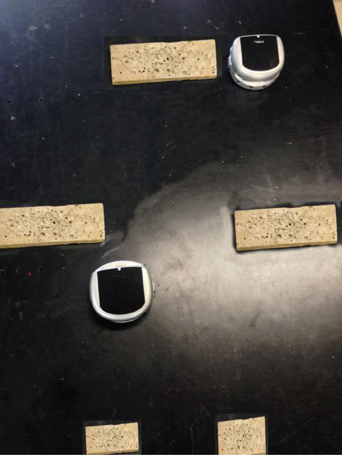
Two agents move to one point.

Fig.2

Position of the Khepera’s UltraSonic sensors.

The Khepera’s sonar readings is defined as l_a,c . It has three degrees, 0, 1, 2, representing the amount of closeness to the nearest obstacle or other agents. 0 indicates for obstacles or agents which are near, 1 indicates for obstacles or agents which are in a medium distance and finally, 2 is for obstacles or agents which are relatively far from the sensors.

The parameters d_a (the distance to the target or the goal) and p_a (the relative angle to the target or goal) are divided in eight degrees (0 -8). Where 0 represents the smallest distance or angle, and 8 represents the greatest relative distance or angle from the current Khepera’s position to the target or goal.

The actions available for the Khepera robot are:

Move forward

Turn in clockwise direction

Turn in counter clockwise direction

Stand-Still

The sensor data are inaccurate and fluctuating. In order to avoid these influences for the reinforcement learning and the Q-iteration, the movement of the robots are relatively slow during the learning process. The collisions with other objects or agent are reduced [37].

The state is defined as x = [x_1,x₂, . . ., x₈] ^T . Each agent has the coordinates in two-dimension positions, s_ix and s_iy, and velocities in two dimensions, ${\dot{s}}_{ix}$ and ${\dot{s}}_{iy} .$ So $x = {[s_{1 x}, s_{1 y,} {\dot{s}}_{1 x}, {\dot{s}}_{1 y}, s_{2 x}, s_{2 y,} {\dot{s}}_{2 x}, {\dot{s}}_{2 y}]}^{T}$

The continuos time dynamics of the agents are $\begin{matrix} {\ddot{s}}_{1 x} & = & - η (s_{1 x}, s_{1 y}) \frac{{\dot{s}}_{1 x}}{m_{1}} + \frac{u_{1 x}}{m_{1}} \\ {\ddot{s}}_{1 y} & = & - η (s_{1 x}, s_{1 y}) \frac{{\dot{s}}_{1 y}}{m_{1}} + \frac{u_{1 y}}{m_{1}} \\ {\ddot{s}}_{2 x} & = & - η (s_{2 x}, s_{2 y}) \frac{{\dot{s}}_{2 x}}{m_{2}} + \frac{u_{2 x}}{m_{2}} \end{matrix}$ (19) ${\ddot{s}}_{2 y} = - η (s_{2 x}, s_{2 y}) \frac{{\dot{s}}_{2 y}}{m_{2}} + \frac{u_{2 y}}{m_{2}}$ where η (s_ix, s_iy) is the friction which depends on the position of each agent, the control signal is U = [u_1x, u_1y, u_2x, u_2y] ^T which is a force, m_i is the mass of each robot.

The aim of the Q-iteration algorithm is to obtain the transition function f. The continuos time system is discretized with a step T = 0.4 s. The dynamics of the system are integrated between the sampling time. The start points are selected randomly. The training iteration is 1000 . If the final goal is not accomplished within 1000 iteration, the experiment is restarted. The magnitude of the state and action variables are bounded and normalized as: s_ix and s_iy ∈ [- 6, 6] meters, ${\dot{s}}_{ix}$ and ${\dot{s}}_{iy} \in [- 3, 3] \frac{m}{s}$ . The force is bounded as u_ix, u_ix ∈ [- 2, 2] for i = 1, 2. The friction coefficient is $η = 1 \frac{kg}{s}$ , the mass of the agent is m = 0.5 kg.

The control actions for each agent are discrete with 25 levels: U_i = [-2 - 0.2 0 0.2 2] × [-2 - 0.2 0 0.2 2], i = 1, 2. They correspond to force in diagonal, left, right, up, down and no force applied.

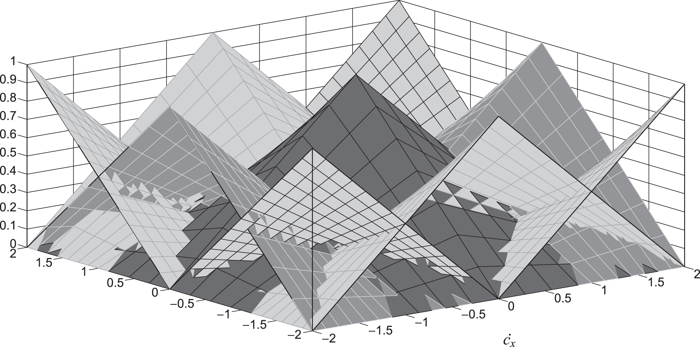
The membership functions used for the position state and velocity state are triangular, see Fig. 3 [39]. The cores of the membership function for the position domain s is centred at [-6, - 3, - 0.3, - 0.1, 0, 0.1, 0.3, 3, 6] . The cores of the membership function for the velocity domain are: [-3, - 1, 0, 1, 3]. There are 50625 pairs (x, u) to approximate each agent in the vector parameter φ. This amount increases with the number of membership functions. The partition of the state space x is determined by the product of the individual membership function for each agent $μ (x) = \prod_{i = 1}^{2} μ_{s_{ix}} \prod_{i = 1}^{2} μ_{s_{iy}} \prod_{i = 1}^{2} μ_{{\dot{s}}_{ix}} \prod_{i = 1}^{2} μ_{{\dot{s}}_{iy}}$ (20)

Fig.3

Triangular fuzzy partition for velocities in X and Y.

The final objective is the agents arrive at the same time in minimum time by the reward function ρ $\begin{array}{l} ρ (x, u) = 5 if ‖ x ‖ < 0.1 \\ ρ (x, u) = 0 in another way \end{array}$ (21) $ρ (x, u) = 0 in another way$

For the coordination problem, the agents consider each other. They do not use explicit coordination conditions for the other agents. They use explicit coordination or negotiation like social conventions, roles and communication [38]. So our algorithm accomplish an implicit form of coordination where the agents learn to prefer on the equally good solutions. 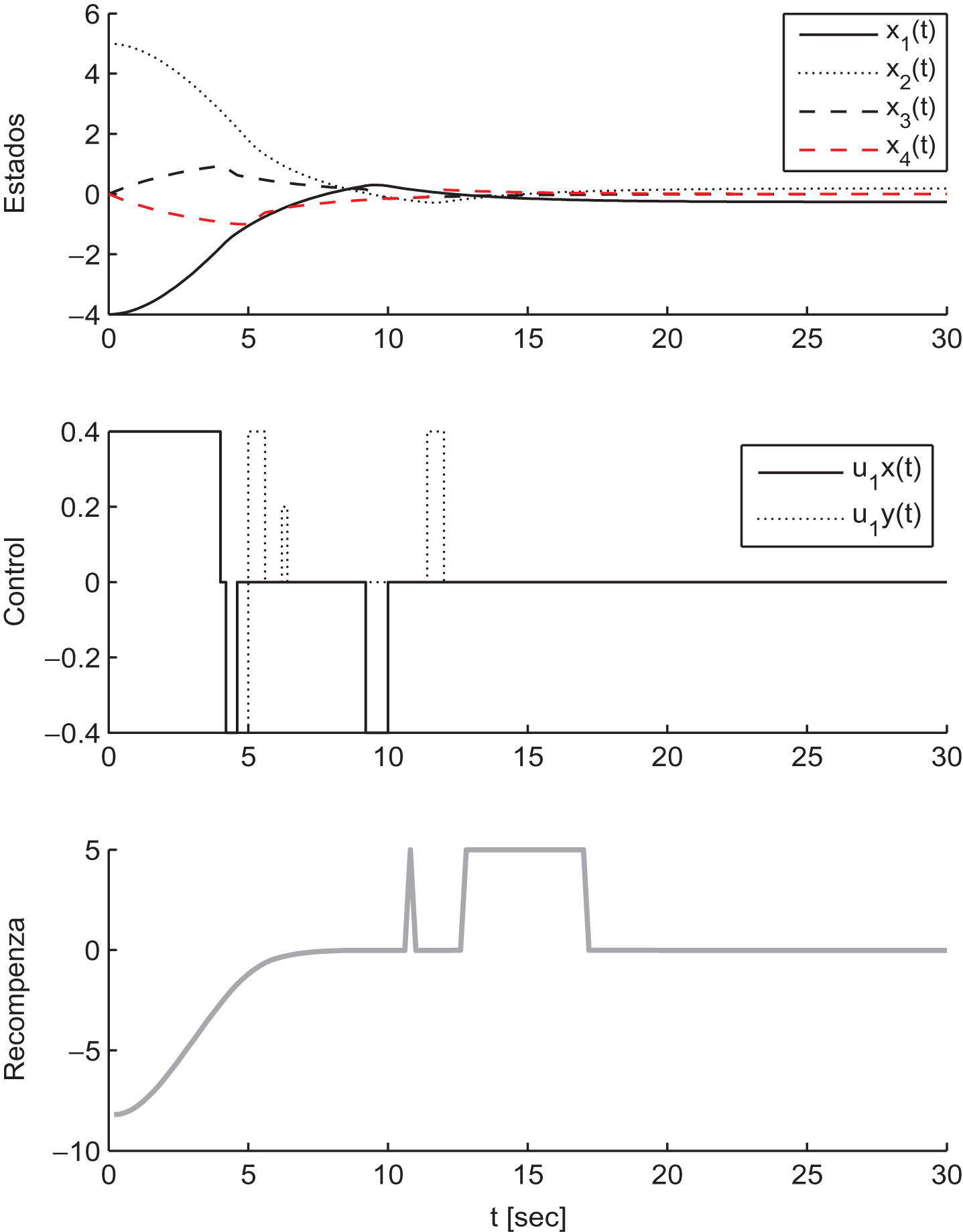After the Q-iteration is performed, φ^∗ is obtained which is a policy can be derived by a interpolation between a the best local action for each agent $h_{i}^{*} (x) = \sum_{d = 1}^{N} φ_{i, d} (x) u_{j_{id}^{*}}$ (22) where $j_{i, d}^{*} \in arg max F (φ^{*}) (x, u) .$

In our experiment the discount factor is γ = 0.96, the threshold is ξ = 0.05, the initial conditions for the experiment is s₀ = [-4, - 6, - 2, 2, 5, 3, 2, - 1] . The control signal U₁ = [u_1x, u_1y] and the states of Agent-1 is shown in Fig. 4. Figure 5 shows the results of Agent-2. We can see that they converge after 310 iterations.

Fig.4

States of Agent 1 (second - meter).

Fig.5

States of Agent 2 (second - meter).

The vector approximation parameter φ converges after 330 iterations, the bounded ||φ_l+1 - φ_l|| ≤ ξ is reached. The final path are showed in Fig. 6. It is evidently different from the optimal policy, which should drive both agents in a straight line toward the goal.

Fig.6

Final path by Agent 1 and Agent 2 (meter - meter).

Now we use Gaussian membership functions $μ (t) = exp (- \frac{{[x (t) - c]}^{2}}{σ^{2}})$ (23) where the center c ∈ [- 3, 3], σ are selected randomly from 1.5 to 2.5 .

The two robot are on a tennis court, see Fig. 7. In this experiment the discount factor is γ = 0.8, the threshold is ξ = 0.05m, the initial conditions for the experiment is s₀ = [-10, - 12, - 7, 16, 21, 11, 13, - 4] . The control signal U₁ = [u_1x, u_1y] and the states of Agent-1 is shown in Fig. 8. Figure 9 shows the results of Agent-2. We can see that they can converge after 250 iterations in Fig. 10.

Fig.7

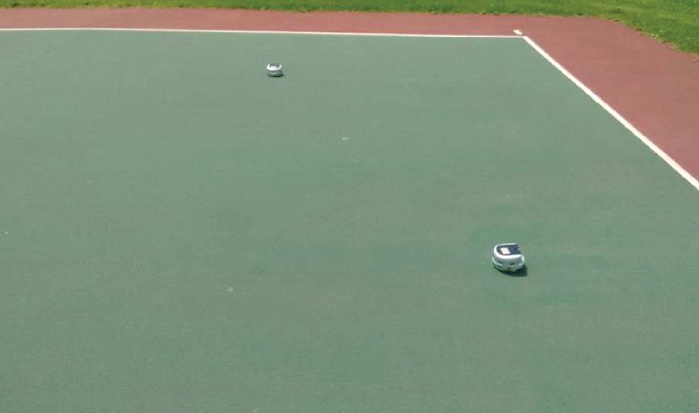
Two agents move on a tennis court.

Fig.8

States and signal control for the Agent 1 (second - meter).

Fig.9

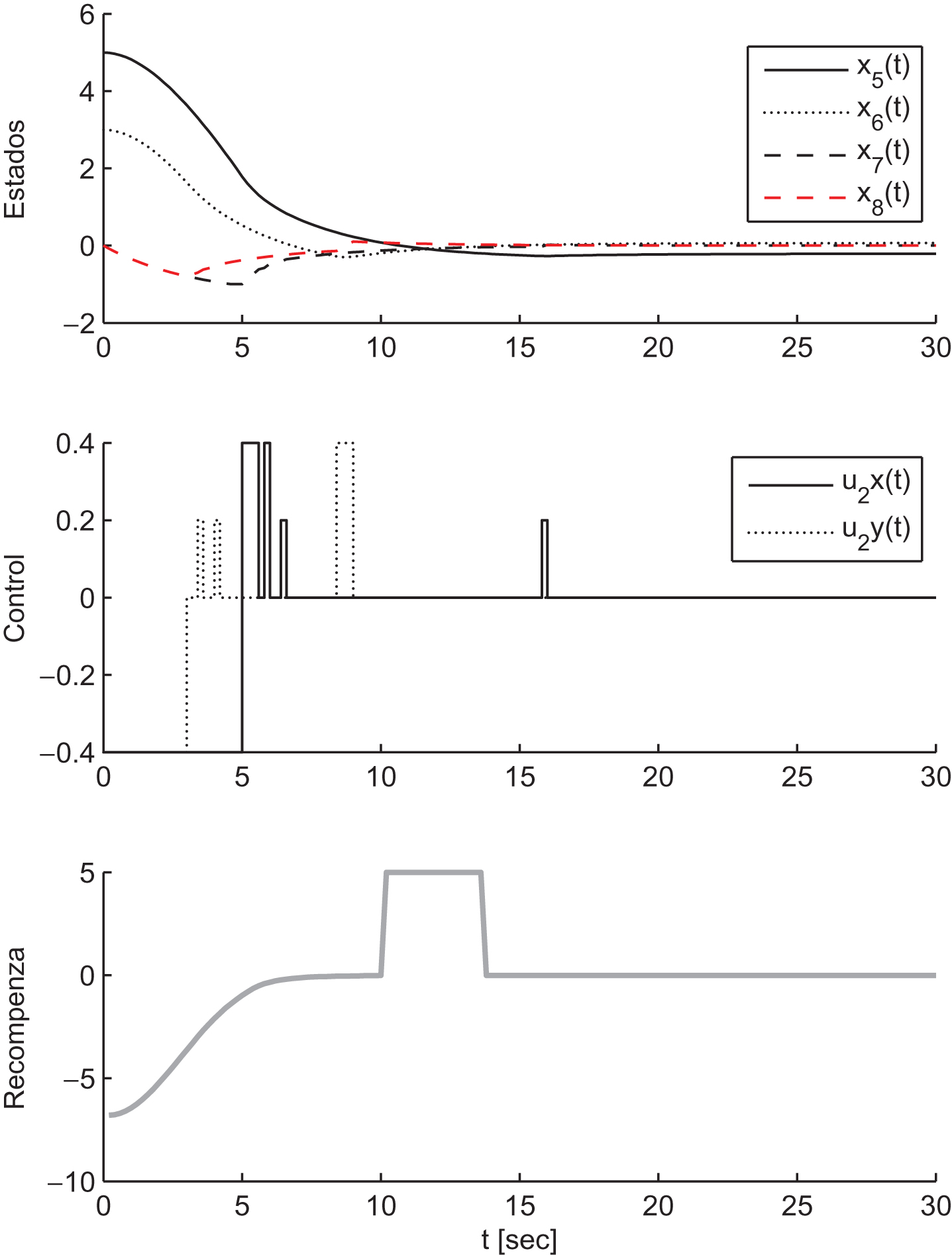
States and signal control for the Agent 2 (second - meter).

Fig.10

Final path by Agent 1 and Agent 2 (meter - meter).

The conclusion the triangle functions are more simple, while the Gaussian functions are more effective.

Now we compare our fuzzy Q-iteration with the classical Q-iteration. Because the classicalQ-iteration can be only applied to discrete-time learning, the tennis court is gridded with 7 × 8 cells. The initial position of the two agents are the same as above. Each time, they can move one cell. They will stop if the target cell is arrived. The object is the two robot reach the target at the same time. After 24 trainings trial the Q-tables converge to the Q-values, see Fig. 11.

Fig.11

Performance of the Q- learning.

The learning time is similar as the fuzzyQ-iteration, however the accuracy is the dimension of one cell. It is about 30 cm. The accuracy of fuzzy Q-iteration is the threshold ξ = 5 cm. If the classical Q-iteration wants to obtain the same accuracy, the grid should be 42 × 48, the training time is 6 times more. These results are shown in Table 1.

Table 1

Training time and accuracy of RL

Training	56 cells		2016 cells
	Classical	Fuzzy	Classical	Fuzzy
Error (cm)	30	5.2	5	3.5
Time (second)	23	24	160	25

We can see that, for this tennis court RL problem, 56 cells is good enough for our fuzzy RL algorithm. Both training error and training time are acceptable. However, for the classical RL, the training error is very big (30 cm). We have to use more cells (2016 cells) to improve training accuracy of the classical RL. Now the training time of the classical RL is much more (160 seconds).

4 Conclusion

In this paper we presents a fuzzy Q-iteration to modify WoLF-PHC algorithm. This fuzzy reinforcement learning can handle multi agent path planning problem in continuous state space. The fuzzy quantization of the states and joint action minimizes the convergence time and avoids huge storage for Q-values and Q-table. The convergence and existence of the algorithm are also proven.

The performance of the fuzzy reinforcement learning is studied by two mobile Khepera robots. The experimental results show the effectiveness of the new path planning method for the multi agents. Future work is to extend this method for model free agents, who can learn itself dynamics in the environment or in the stochastic dynamics.

References

Sen

and Weiss

, Multiagent Systems: A Modern Approach to Distributed Artificial Intelligence, MIT PressCambridge.

Stone

and Veloso

, Multiagent systems: A survey from machine learning perspective, Autonomus Robots8(3) (2000), 345–383.

Wooldridge An Introduction to MultiAgent Systems, John Wiley & Sons, 2002.

Kaelbling

L.P.

, Littman

M.L.

and Moore

A.W.

, Reinforcement learning: A survey, Journal of Artificial Intelligence Research4(1) (1996), 237–285.

Arel

, Liu

, Urbanik

and Kohls

A.G.

, Reinforcement learning-based multi-agent system for network traffic signal control, IET Intelligent Transport Systems4(2) (2010), 128–135.

Cherkassky

and Mulier

, Learning from data: Concepts, Theory and Methods, Wiley-IEEE Press, Chichester, 1998.

Sejnowski

T.J.

and Hinton

, Unsupervised Learning: Foundations of Neural Computation, MIT Press, 1999.

and Wang

, Consensus of linear multi-agent systems subject to actuator saturation, International Journal of Control, Automation, and Systems11(4) (2013), 649–656.

Cruz

D.L.

and Yu

, Multi-Agent Path Planning in Unknown Environment with Reinforcement Learning and Neural Network, 2014 IEEE International Conference on Systems, Man, and Cybernetics (SMC14), San Diego, USA, 2014, pp. 3469–3474.

10.

Abul

, Polat

and Alhajj

, Multi-agent reinforcement learning using function approximation, IEEE transactions on Systems, Man and Cybernetics Part C: Applications and Reviews (2000), 485–497.

11.

Fernandez

and Parker

L.E.

, Learning in large cooperative multirobots systems, International Journal of Robotics and Automatization, Special Issue on Computational Intelligence Techniques in Cooperative Robots16(4) (2001), 217–226.

12.

Tamakoshi

and Ishi

, Multi agent reinforcement learning applied to a chase problem in a continuos world, Artifitial Life and Robotics5(4) (2001), 202–206.

13.

Ishiwaka

, Sato

and Kakazu

, An approach to persuit problem on a heterogeneous multiagent system using reinforcement learning, Robotics and Autonomous Systems43(4) (2003), 245–256.

14.

Bowling

and Veloso

, Multiagent learning using a variable learning rate, Artificial Intelligence136(2) (2002), 215–250.

15.

Fathinezhad

, Derhami

and Rezaeian

, Supervised fuzzy reinforcement learning for robot navigation, Applied Soft Computing40 (2016), 33–41.

16.

Boutilier

, Planning, Learning and Coordination in Multiagent Decision Processes, In Proceedings of the Sixth Conference on Theoretical Aspects of Rationality and Knowledge (TARK96), 1996, pp. 195–2102.

17.

Harsanyi

J.C.

and Selten

, A General Theory of Equilibrium Selection in Games, MIT Press, Cambridge, 1988.

18.

Busoniu

, Babuska

and De Schutter

, Multi-agent Reinforcement Learning: An Overview, Innovation in MASs and Applications. SCI 310, Springer VerlagBerlin Heidelberg, pp. 183–221.

19.

Basar

and Olsder

G.J.

, Dynamic Noncooperative Game Theory, 2nd edition. Society for Andustrial and Applied Mathematics, SIAM, 1999.

20.

Busoniu

, De Schutter

and Babuska

, Decentralized Reinforcement Learning Control of a robotic Manipulator, International Conference on Control, Automation, Robotics and Vision, 2006, I CARCV ’06. 9th.

21.

Bertsekas

D.P.

, Dynamic Programming and optimal control vol 2, third edition, Athena Scientific.

22.

Istratesku

, Fixed Point Theory: An introduction Springer, 2002.

23.

Melo

F.S.

, Meyn

S.P.

and Ribeiro

M.I.

, An analysis of reinforcement learning with functions approximation, Proceedings 25th International Conference on Machine Learning (ICML-08), Helsinky, Finland, 2008, pp. 664–671.

24.

Szepesvari

Cs.

and Smart

W.D.

, Interpolation baes Q-learning, Procedings 21st International Conference on Machine Learning (ICML-04), Bannf, Canada, pp. 791–798.

25.

Sutton

R.S.

, McAllester

D.A.

, Singh

S.P.

and Mansour

, Policy gradient methods for reinforcement learning with function approximation, Advances in Neural Information Processing Systems 12, MIT Press, 2000, pp. 1057–1063.

26.

Bertsekas

D.P.

and Tsitsiklis

J.N.

, Neuro-dynamic programming, Athena Scientific, 1996.

27.

Tsitsiklis

J.N.

and Van Roy

, Feature-based methods for large scale dynamic programming, Machine Learning22(1– 3) (1996), 59–94.

28.

Mamdani

, Application of fuzzy logic to approximate reasoning using linguistic systems, IEEE Transactions on Computers26 (1977), 1182–1191.

29.

Kruse

, Gebhardt

J.E.

and Klowon

, Foundations of Fuzzy Systems, Wiley, 1994.

30.

Gordon

G.J.

, Reinforcement learning with function approximation converges to a region. In Leen

T.K.

, Dietterich

T.G.

and Tresp

, editors, Advances in Neural Information Processing Systems 13, MIT Press, 2001, pp. 1040–1046.

31.

Tsitsiklis

J.N.

, Asynchronous stochastic approximation and Qlearning, Machine Learning16(1) (1994), 185–202.

32.

Berenji

H.R.

and Khedkar

, Learning and tuning fuzzy logic controllers through reinforcements, IEEE Transactions on Neural Networks3(5) (1992), 724–740.

33.

Munos

and Moore

, Variable-resolution discretization in optimal control, Machine Learning49(2– 3) (2002), 291–323.

34.

Chow

C.-S.

and Tsitsiklis

J.N.

, An optimal one-way multigrid algorithm for discrete-time stochastic control, IEEE Transactions on Automatic Control36(8) (1991), 898–914.

35.

Busoniu

, Ernst

, De Schutter

and Babuska

, Approximate dynamic programming with fuzzy parametization, Automatica46 (2010), 804–814.

36.

K-team Corporation, 2013http://www-k-team.com

37.

Ganapathy

, Yun

S.C.

and Lui

W.L.D.

, Utilization of webots and Khepera II as a Platform for neural Q-learning controllers, IEEE Symposium on Industrial Electronics and Applications (ISIEA 2009), Kuala Lumpur, Malaysia.

38.

Vlassis

, A concise Introduction to Multi Agent Systems amd Distributed Artificial Intelligence. Synthesis Lectures in Artificial Intelligence and Machine Learning. Morgan & Claypool Publishers, 2007.

39.

Busoniu

, Ernst

, Schutter

and Babuska

, Continuous-State Reinforcement Learning with Fuzzy Approximation, Adaptive Agents and MAS III, Springer-VerlagBerlin Heidelberg, Tuyls

et al. (Eds.), LNAI 48652008, pp. 27–43.