The relationship between L -subuniverses and L -convexities

1 Introduction

In the standard case, a set in an n-dimensional Euclidean space is convex if and only if it contains the whole segments joining each two of its points. By axiomatizing the properties of convex sets in Euclidean spaces, a concept of convexity (or abstract convexity) was introduced in [3, 19]. Since the early decades of last century, the notion of convexity had been redefined by some authors [5, 12]. In this paper, we focus on the convexity with domain finiteness. In [7], Hammer showed that domain finiteness is equivalent to the property that the convexity is closed under totally ordered unions.

A convexity with domain finiteness (also called convexity in [20]) on a non-empty set X is defined to be a family C of 2 ^X which contains ∅, X and which is closed under arbitrary intersections and totally ordered unions (see Definition 2.13). In recent years, the theory of universal algebras [1, 22] has enjoyed a particularly explosive growth. One of the aims of universal algebras is to extract the common elements of several different types of algebraic structures, such as groups, rings, lattices and so on. The relationship between algebraic lattices and subuniverses plays an important part in the theory of universal algebras. In fact, a convexity is an algebraic lattice and each algebraic lattice is isomorphic to a convexity on some set [20].

With the development of fuzzy mathematics, the notion of convexity has already been extended to fuzzy set theory. In 1994, M.V. Rosa presented the notion of fuzzy convexity in [15]. In 2009, Y. Maruyama generalized it to L-fuzzy setting in [13]. More recently, F.G. Shi and Z.Y. Xiu [18] gave a new approach to fuzzification of convexity in a completely different direction and proposed the concept of M-fuzzifying convexity. What’s more, F.G. Shi and E.Q. Li [17] showed that there is a one-to-one correspondence between M-fuzzifying restricted hull operators and M-fuzzifying convexities. And X.Y. Wu and S.Z. Bai introduced M-fuzzifying JHC convex structures and M-fuzzifying Peano interval spaces [23]. Besides, from the perspective of category theory, B. Pang and F.G. Shi [14] discussed some relationships among several types of L-convex spaces, including stratified L-convex spaces, convex-generated L-convex spaces, weakly induced L-convex spaces and induced L-convex spaces.

This paper is organized as follows. In Section 2, some necessary concepts of complete Heyting algebras, universal algebras and L-convex spaces are recalled. In Section 3, the notion of subuniverses in the universal algebra theory is generalized to L-fuzzy setting. Then several equivalent characterizations and some representations of L-subuniverses are given. In Section 4, the relationship between L-subuniverses and L-convexities is discussed in detail. Actually, there is a one-to-one correspondence between L-subuniverses with the smallest L-subset and induced L-convexities.

2 Preliminaries

Throughout this paper, unless otherwise stated, (L, ∨, ∧) denotes a complete Heyting algebra (or a complete frame), where finite meets distribute over arbitrary joins, i.e., a ∧ (⋁ _i∈Ib _i ) = ⋁ _i∈I (a ∧ b _i ) holds for all a, b _i  ∈ L  (i ∈ I). The smallest element and the largest element in L are denoted by ⊥ and ⊤, respectively. Let X be a non-empty set. We denote the set of all subsets (resp., all finite subsets) of X by 2 ^X (resp., 2 fin X ) and denote the set of all L-fuzzy sets of X by L ^X . The smallest element and the largest element in L ^X are denoted by χ_∅ and χ _X , respectively. L ^X is also a complete Heyting algebra when it inherits the structure of the lattice L in a natural way, by defining ∨, ∧, ≤ pointwisely. We often do not distinguish a crisp subset A of X from its characteristic function χ _A . Also, we adopt the convention that ⋀∅ = ⊤ and ⋁∅ = ⊥.

From the definition of complete Heyting algebras, we have the following corollary.

Corollary 2.1. A lattice L is a complete Heyting algebra if and only if it satisfies the following condition: ( ⋁ i 1 ∈ I 1 a i 1 ) ∧ ⋯ ∧ ( ⋁ i n ∈ I n a i n ) = ⋁ ( i 1 , . . . , i n ) ∈ I 1 × ⋯ × I n ( a i 1 ∧ ⋯ ∧ a i n ) , for each n ∈ ℕ and for all {a _{i k} } _{i k ∈I k}  ⊆ L, k = 1, ..., n.

Proof. We first show that the result holds for n = 2. By the definition of complete Heyting algebras, we have (⋁ _i1∈I1a _{i 1} ) ∧ (⋁ _i2∈I2a _{i 2} ) = ⋁ _i2∈I2 ((⋁ _i1∈I1a _{i 1} ) ∧ a _{i 2} )   =   ⋁ _{(i1,i2)∈I1×I2} (a _{i 1}   ∧  a _{i 2} ). Recursively, the result holds for each n ∈ ℕ . □

By Corollary 2.1, it is easy to obtain the following proposition.

Proposition 2.2. Let (L, ∨, ∧) be a complete Heyting algebra. If {A _i  ∣ i ∈ I} ⊆ L ^X is non-empty and totally ordered, then for all finite elements x₁, ..., x _n  ∈ X, ( ⋁ i ∈ I A i ( x 1 ) ) ∧ ⋯ ∧ ( ⋁ i ∈ I A i ( x n ) ) = ⋁ i ∈ I ( A i ( x 1 ) ∧ ⋯ ∧ A i ( x n ) ) .

Proof. We only need to show that (⋁ _i∈IA _i  (x₁)) ∧ (⋁ _i∈IA _i  (x₂)) = ⋁ _i∈I (A _i  (x₁) ∧ A _i  (x₂)) for any x₁, x₂ ∈ X. On one hand, it is obvious that (⋁ _i∈IA _i  (x₁)) ∧ (⋁ _i∈IA _i  (x₂)) ≥ ⋁ _i∈I (A _i  (x₁) ∧ A _i  (x₂)). On the other hand, (⋁ _i∈IA _i  (x₁)) ∧ (⋁ _i∈IA _i  (x₂)) = (⋁ _i∈IA _i  (x₁)) ∧ (⋁ _j∈JA _j  (x₂)) = ⋁ _(i,j)∈I×I  (A _i  (x₁) ∧ A _j  (x₂)). Since {A _i  ∣ i ∈ I} ⊆ L ^X is totally ordered, suppose that A _j  ≤ A _i , we have ⋁_(i,j)∈I×I (A _i  (x₁) ∧ A _j  (x₂)) ≤ ⋁ _i∈I (A _i  (x₁) ∧ A _i  (x₂)). Recursively, the equality holds for any finite elements x₁, ..., x _n  ∈ X. □

An element a in L is called a prime element if b ∧ c ⩽ a implies b ⩽ a or c ⩽ a. An element a in L is called a co-prime element if b ∨ c ⩾ a implies b ⩾ a or c ⩾ a [6]. The set of non-unit (L removes the largest element) prime elements in L is denoted by P (L). The set of non-zero (L removes the smallest element) co-prime elements in L is denoted by J (L).

We say that a is wedge below b (in symbols, a ≺ b), if for every subset D ⊆ L, ⋁D ≥ b implies a ≤ d for some d ∈ D [4]. We denote β (a) = {x ∈ L ∣ x ≺ a} and a ≺  ^op b means that if for every subset D ⊆ L, ⋀D ≤ b implies d ≤ a for some d ∈ D. We denote α (a) = {x ∈ L ∣ x ≺  ^op a}.

For any A ∈ L ^X and a ∈ L, we can define two cut sets of A as follows: A_[a] = {x ∈ X ∣ A (x) ≥ a} and A^(a) = {x ∈ X ∣ A (x) ≰ a}. In the sequel, the binary relation ≺ in L can be used to define two new cut sets of A.

Definition 2.3. [16] Let A ∈ L ^X and a ∈ L. Define A [ a ] = { x ∈ X ∣ A ( x ) ≥ a } , A ( a ) = { x ∈ X ∣ a ∈ β ( A ( x ) ) } , A [ a ] = { x ∈ X ∣ a ∉ α ( A ( x ) ) } , A ( a ) = { x ∈ X ∣ A ( x ) ≰ a } .

Some properties of these cut sets can be found in [9, 16].

Remark 2.4. When L = [0, 1], A_(a) = A^(a) = {x ∈ X ∣ A (x) > a} and A_[a] = A^[a]. But for a general complete lattice L, A_(a), A^(a) and {x ∈ X ∣ A (x) > a} are different. For example, let X = {1, 2, 3} and L = 2^{a,b}. Consider an L-fuzzy set A defined by A (1) = {a, b}, A (2) = {a} and A (3) = {b}. It is easy to check that A_[{a}] = A_({a}) = {1, 2}, A^[{a}] = A^({a}) = {1, 3} and {x ∈ X ∣ A (x) > a} = {1}.

In what follows, some notions and results in the theory of universal algebras are recalled.

We denote X⁰ = {∅} and X ⁿ as the set of n-tuples of elements from X. An operation f : X ⁿ  ⟶ X is called an n-ary operation on X and n is called the arity (or rank) of f. A finitary operation is an n-ary operation, for some n. An operation f is called a nullary operation if its arity is zero, it is determined by the image f (∅).

Definition 2.5. [1, 2] Let X be a non-empty set and F be a family of finitary operations on X. Then 〈 X , F 〉 is called an algebra of type F and the set X is usually called the universe (or underlying set) of 〈 X , F 〉 .

We denote F n (resp., F 0 ) as the set of all n-ary operations (resp., all nullary operations). If F is finite, say F = { f 1 , . . . , f k } , we often write 〈X, f₁, ..., f _k 〉 for 〈 X , F 〉 , usually adopting the convention: arity f₁≥ arity f₂≥ ⋯ ≥ arity f _k .

Example 2.6. A lattice is an algebra 〈L, ∨, ∧ 〉 with two binary operations satisfying the following conditions. ∀a₁, a₂, a₃ ∈ L,

a₁ ∨ a₂ = a₂ ∨ a₁, a₁ ∧ a₂ = a₂ ∧ a₁;

Example 2.7. A group is an algebra 〈G, ·, ^-1, 1〉 with a binary, a unary and a nullary operation in which the following identities are true. ∀a, a₁, a₂, a₃ ∈ G,

a₁ · (a₂ · a₃) = (a₁ · a₂) · a₃;

A group is Abelian (or commutative) if the following identity is true.

a₁ · a₂ = a₂ · a₁.

A semigroup is a groupoid 〈G, · 〉 in which (G1) is true.

Example 2.8. A ring is an algebra 〈R, +, ·, -, 0〉, where + and · are binary, - is unary and 0 is nullary, satisfying the following conditions. ∀a₁, a₂, a₃ ∈ R,

〈R, +, -, 0〉 is an Abelian group;

Definition 2.9. [1, 2] Let 〈 X , F 〉 be an algebra of type F . A ∈ 2 ^X is called a subuniverse of 〈 X , F 〉 if it is closed under all operations of 〈 X , F 〉 , namely, for each n ∈ ℕ and for all f ∈ F n , x₁, ..., x _n  ∈ A, we have f (x₁, ..., x _n ) ∈ A.

We denote S 〈 X , F 〉 as the set of all subuniverses of 〈 X , F 〉 .

Remark 2.10. The empty set ∅ may be a subuniverse. If F 0 = ∅ , then ∅ is a subuniverse. If F 0 ≠ ∅ , then ∅ is not a subuniverse.

Definition 2.11. [1, 2] Given an algebra 〈 X , F 〉 of type F . For each A ∈ 2 ^X , define an operator sg : 2 ^X  ⟶ 2 ^X by sg ( A ) = ⋂ { B ∣ A ⊆ B ∈ S 〈 X , F 〉 } . Then sg (A) is called the subuniverse generated by A.

Theorem 2.12. [1, 2] Let 〈 X , F 〉 be an algebra of type  F . Then sg (A) is the minimum subuniverse including A and sg ( A ) = ⋃ k = 0 ∞ E k ( A ) , where E⁰ (A) = A, E k + 1 ( A ) = E k ( A ) ⋃ { f ( x 1 , . . . , x n ) ∣ ∃ n ∈ ℕ , f ∈ F n , x 1 , . . . , x n ∈ E k ( A ) } .

Convexities (or convex structures) exist in various research areas, such as, vector spaces, partially ordered sets, semilattices, lattices, matroids and so on. Subuniverses have close relations with convexities. In fact, it is not difficult to find that all subuniverses of some algebra with the empty set can constitute an convexity.

Definition 2.13. [20] A subset C of 2 ^X is called a convexity, if it satisfies the following conditions:

∅, X ∈ C ;

The pair ( X , C ) is called a convex space. The members of C are called convex sets. For any A ∈ 2 ^X , co C ( A ) = ⋂ { C ∣ A ⊆ C ∈ C } is called convex hull of A, which is the smallest convex set that contains A. Moreover, co C : 2 X ⟶ 2 X , A ↦ co C ( A ) can alternatively be regarded as an operator called (convex) hull operator which have the normalization, extensive, idempotent and domain finite laws. That is,

co (∅) = ∅;

Actually, there exists a one-to-one correspondence between convexities and operators with the properties (CO1)-(CO3) and (DF) [20].

In 1994, M.V. Rosa introduced the concept of fuzzy convexity in [15]. In 2009, Y. Maruyama generalized it to L-fuzzy setting as follows.

Definition 2.14. [13] A subset C of L ^X is called an L-convexity if it satisfies the following conditions:

χ_∅, χ X ∈ C ;

The pair ( X , C ) is called an L-convex space and the members of C are called L-convex sets. For each A ∈ L ^X , co C ( A ) = ⋀ { C ∣ A ≤ C ∈ C } is called the L-convex hull of A.

3 L-subuniverses and their characterizations

In this section, the notion of subuniverses in the theory of universal algebras is generalized to L-fuzzy setting, which is called L-subuniverses. Then several equivalent characterizations and representations of L-subuniverses are given.

Definition 3.1. Let 〈 X , F 〉 be an algebra of type F . A ∈ L ^X is called an L-subuniverse of 〈 X , F 〉 if for each n ∈ ℕ and for all f ∈ F n , x₁, ..., x _n  ∈ X, we have A (x₁) ∧ ⋯ ∧ A (x _n ) ≤ A (f (x₁, ..., x _n )).

We denote LFS 〈 X , F 〉 as the set of all L-subuniverse of 〈 X , F 〉 .

Remark 3.2. If F 0 = ∅ , then χ_∅ is an L-subuniverse. If F 0 ≠ ∅ , then χ_∅ is not an L-subuniverse.

Example 3.3. Let an algebra be a lattice 〈L, ∨, ∧ 〉 which has no nullary operations. Then F 0 = ∅ and χ_∅ is an L-subuniverse. Let an algebra be a group 〈G, ·, ^-1, 1〉 which has a binary, a unary and a nullary operation. Then F 0 = { f } . By Definition 3.1, we know ⋀∅ = ⊤ ≰ χ_∅ (f (∅)) = χ_∅ (1) = ⊥. Hence χ_∅ is not an L-subuniverse. Let an algebra be a bounded lattice 〈L, ∨, ∧, 0, 1〉 which has two binary and two nullary operations. Then F 0 = { f , g } and χ_∅ is not an L-subuniverse as well.

Theorem 3.4. L-subuniverse1 Let 〈 X , F 〉 be an algebra of type F and A ∈ L ^X . Then the following statements are equivalent.

A is an L-subuniverse of 〈 X , F 〉 .

Proof. (1) ⇒ (2). Assume that A is an L-subuniverse of 〈 X , F 〉 . For each a ∈ L and for all x₁, ..., x _n  ∈ A_[a], we have A (f (x₁, ..., x _n )) ≥ A (x₁) ∧ ⋯ ∧ A (x _n ) ≥ a. This implies f (x₁, ..., x _n ) ∈ A_[a]. Hence A_[a] is a subuniverse of 〈 X , F 〉 .

(2) ⇒ (1) Suppose that A_[a] is a subuniverse of 〈 X , F 〉 for each a ∈ L. For each n ∈ ℕ and for all f ∈ F n , x₁, ..., x _n  ∈ X. Let a = A (x₁) ∧ ⋯ ∧ A (x _n ). Then x₁, ..., x _n  ∈ A_[a]. So A (f (x₁, ..., x _n )) ∈ A_[a]. Hence A (f (x₁, ..., x _n )) ≥ a = A (x₁) ∧ ⋯ ∧ A (x _n ), which means A is an L-subuniverse of 〈 X , F 〉 . □

In order to discuss other characterizations of L-subuniverses, we need to recall some results in completely distributive lattices.

Lemma 3.5. [21] Let L be a completely distributive lattice and let {a _i  ∣ i ∈ I} ⊆ L. Then

α (⋀ _i∈Ia _i ) = ⋃ _i∈Iα (a _i ), i.e., α (·) : L ⟶ 2 ^X is a ⋀-⋃ mapping.

From Lemma 3.5, we know that α (·) is an order-reversing and β (·) is an order-preserving.

Lemma 3.6. [18] Let L be a completely distributive lattice. Then for all x, y ∈ L, the following conditions are equivalent.

x ⩽ y.

Theorem 3.7. Let 〈 X , F 〉 be an algebra of type F and A ∈ L ^X . If L is completely distributive, then the following conditions are equivalent.

A is an L-subuniverse of 〈 X , F 〉 .

Proof. (1) ⇒ (2) It follows immediately from Theorem 3.4.

(2) ⇒ (1) In order to prove that A is an L-subuniverse of 〈 X , F 〉 , we need to check the inequality A (x₁) ∧ ⋯ ∧ A (x _n ) ≤ A (f (x₁, ..., x _n )) for each n ∈ ℕ and for all f ∈ F n , x₁, ..., x _n  ∈ X. Assume that a ∈ J (L) with a ≤ A (x₁) ∧ ⋯ ∧ A (x _n ). Then a ≤ A (x₁), ..., a ≤ A (x _n ). This implies x₁ ∈ A_[a], ..., x _n  ∈ A_[a]. Note that A_[a] is a subuniverse for each a ∈ J (L). Then f (x₁, ..., x _n )) ∈ A_[a], which means a ≤ A (f (x₁, ..., x _n )). By the arbitrariness of a, we obtain A (x₁) ∧ ⋯ ∧ A (x _n ) ≤ A (f (x₁, ..., x _n )). Hence A is an L-subuniverse of 〈 X , F 〉 .

(1) ⇒ (3) For each a ∈ α (⊥), take any x₁, ..., x _n  ∈ A^[a]. Then a ∉ α (A (x₁)), ..., a ∉ α (A (x _n )). Since α is a ⋀-⋃ mapping, we have a ∉ α (A (x₁)) ∪ ⋯ ∪ α (A (x _n )) = α (A (x₁) ∧ ⋯ ∧ A (x _n )). Note that A is an L-subuniverse. Then A (x₁) ∧ ⋯ ∧ A (x _n ) ≤ A (f (x₁, ..., x _n )) for each n ∈ ℕ and for all f ∈ F n . So α (A (f (x₁, ..., x _n ))) ⊆ α (A (x₁) ∧ ⋯ ∧ A (x _n )). Thus a ∉ α (A (f (x₁, ..., x _n ))). This shows f (x₁, ..., x _n ) ∈ A^[a]. Hence A^[a] is a subuniverse of 〈 X , F 〉 .

(3) ⇒ (1) We need to check the inequality A (x₁) ∧ ⋯ ∧ A (x _n ) ≤ A (f (x₁, ..., x _n )) for each n ∈ ℕ and for all f ∈ F n , x₁, ..., x _n  ∈ X. Assume that a ∈ α (⊥) with a ∉ α (A (x₁) ∧ ⋯ ∧ A (x _n )). Since α (A (x₁) ∧ ⋯ ∧ A (x _n )) = α (A (x₁)) ∪ ⋯ ∪ α (A (x _n )), we know a ∉ α (A (x₁)), ..., a ∉ α (A (x _n )), which means x₁, ..., x _n  ∈ A^[a]. Note that A^[a] is a subuniverse for each a ∈ α (⊥). Then A (f (x₁, ..., x _n )) ∈ A^[a]. This shows a ∉ α (A (f (x₁, ..., x _n ))). By the arbitrariness of a, we obtain A (x₁) ∧ ⋯ ∧ A (x _n ) ≤ A (f (x₁, ..., x _n )). Hence A is an L-subuniverse of 〈 X , F 〉 .

(1) ⇒ (4) For each a ∈ P (L), take any x₁, ..., x _n  ∈ A^(a). Then A (x₁) ≰ a, ..., A (x _n ) ≰ a. Since a is a prime element, we have A (x₁) ∧ ⋯ ∧ A (x _n ) ≰ a. Note that A is an L-subuniverse. Then A (x₁) ∧ ⋯ ∧ A (x _n ) ≤ A (f (x₁, ..., x _n )) for each n ∈ ℕ and for all f ∈ F n . It follows that A (f (x₁, ..., x _n )) ≰ a, which shows f (x₁, ..., x _n ) ∈ A^(a). Hence A^(a) is a subuniverse of 〈 X , F 〉 .

(4) ⇒ (1) It suffices to check the inequality A (x₁) ∧ ⋯ ∧ A (x _n ) ≤ A (f (x₁, ..., x _n )) for each n ∈ ℕ and for all f ∈ F n , x₁, ..., x _n  ∈ X. Suppose that a ∈ P (L) with A (x₁) ∧ ⋯ ∧ A (x _n ) ≰ a. Then A (x₁) ≰ a, ..., A (x _n ) ≰ a. This means x₁, ..., x _n  ∈ A^(a). Note that A^(a) is a subuniverse for each a ∈ P (L). Then f (x₁, ..., x _n ) ∈ A^(a), which shows A (f (x₁, ..., x _n )) ≰ a. By the arbitrariness of a, we obtain A (x₁) ∧ ⋯ ∧ A (x _n ) ≤ A (f (x₁, ..., x _n )). Hence A is an L-subuniverse of 〈 X , F 〉 .

(1) ⇒ (5) For each a ∈ β (⊤), take any x₁, ..., x _n  ∈ A_(a). Then a ∈ β (A (x₁)), ..., a ∈ β (A (x _n )). Since β (A (x₁)) ∩ ⋯ ∩ β (A (x _n )) = β (A (x₁) ∧ ⋯ ∧ A (x _n )), we know a ∈ β (A (x₁) ∧ ⋯ ∧ A (x _n )). Note that A is an L-subuniverse. Then A (x₁) ∧ ⋯ ∧ A (x _n ) ≤ A (f (x₁, ..., x _n )) for each n ∈ ℕ and for all f ∈ F n . So β (A (x₁) ∧ ⋯ ∧ A (x _n )) ⊆ β (A (f (x₁, ..., x _n ))). Thus a ∈ β (A (f (x₁, ..., x _n ))). This shows f (x₁, ..., x _n ) ∈ A_(a). Hence A_(a) is a subuniverse of 〈 X , F 〉 .

(5) ⇒ (1) We need to check the inequality A (x₁) ∧ ⋯ ∧ A (x _n ) ≤ A (f (x₁, ..., x _n )) for each n ∈ ℕ and for all f ∈ F n , x₁, ..., x _n  ∈ X. Suppose that a ∈ β (⊤) with a ∈ β (A (x₁) ∧ ⋯ ∧ A (x _n )). Since β (A (x₁) ∧ ⋯ ∧ A (x _n )) = β (A (x₁)) ∩ ⋯ ∩ β (A (x _n )), we have a ∈ β (A (x₁)), ..., a ∈ β (A (x _n )). This shows x₁, ..., x _n  ∈ A_(a). Note that A_(a) is a subuniverse for each a ∈ β (⊤). Then A (f (x₁, ..., x _n )) ∈ A_(a), which implies a ∈ β (A (f (x₁, ..., x _n ))). By the arbitrariness of a, we obtain A (x₁) ∧ ⋯ ∧ A (x _n ) ≤ A (f (x₁, ..., x _n )). Hence A is an L-subuniverse of 〈 X , F 〉 . □

From Definition 3.1, it is not difficult to check that an arbitrary intersection of L-subuniverses of 〈 X , F 〉 is also an L-subuniverse. Hence we have the following definition.

Definition 3.8. Let 〈 X , F 〉 be an algebra of type F . For each A ∈ L ^X , define an operator sg _L  : L ^X  ⟶ L ^X by ∀A ∈ L ^X , sg L ( A ) = ⋀ { B ∣ A ≤ B ∈ LFS 〈 X , F 〉 } .

Then sg _L  (A) is called the L-subuniverse generated by A.

Theorem 3.9. Let 〈 X , F 〉 be an algebra of type F . Then sg _L  (A) is the minimum L-subuniverse including A and LFS 〈 X , F 〉 = { A ∈ L X ∣ sg L ( A ) = A } .

Proof. The proofs are trivial from Definitions 3.1 and 3.8 and omitted here. □

In what follows, we shall give a specific representation of the L-subuniverse generated by A.

Theorem 3.10.Let 〈 X , F 〉 be an algebra of type F . Then sg L ( A ) ( x ) = ⋁ k = 0 ∞ E k ( A ) ( x ) for all A ∈ L ^X and x ∈ X, where E⁰ (A) (x) = A (x) and E k + 1 ( A ) ( x ) = E k ( A ) ( x ) ∨ ( ⋁ { E k ( A ) ( x 1 ) ∧ ⋯ ∧ E k ( A ) ( x n ) | ∃ n ∈ ℕ , f ∈ F n , x 1 , . . . , x n ∈ X , x = f ( x 1 , . . . , x n ) } ) for each k ∈ ℕ .

Proof. Denote C ( x ) = ⋁ k = 0 ∞ E k ( A ) ( x ) , we need to prove that C is the minimum L-subuniverse including A.

(i) From the above recurrence formula, it is easy to see that A≤ E (A) ≤ E² (A) ≤ ⋯, which means A ≤ E ^k  (A) for each k ∈ ℕ and { E k ( A ) ∣ k ∈ ℕ } is an increasing sequence. This shows A ≤ C.

(ii) In order to prove C is an L-subuniverse, we need to show that C (x₁) ∧ ⋯ ∧ C (x _n ) ≤ C (f (x₁, ..., x _n )) for each n ∈ ℕ and for all f ∈ F n , x₁, ..., x _n  ∈ X. By Proposition 2.2, we have C ( x 1 ) ∧ ⋯ ∧ C ( x n ) = ( ⋁ k = 0 ∞ E k ( A ) ( x 1 ) ) ∧ ⋯ ∧ ( ⋁ k = 0 ∞ E k ( A ) ( x n ) ) = ⋁ k = 0 ∞ ( E k ( A ) ( x 1 ) ∧ ⋯ ∧ E k ( A ) ( x n ) ) .

Since C ( f ( x 1 , . . . , x n ) ) = ⋁ k = 0 ∞ E k ( A ) ( f ( x 1 , . . . , x n ) ) , where E⁰ (A) = A and E k + 1 ( A ) ( f ( x 1 , . . . , x n ) ) = E k ( A ) ( f ( x 1 , . . . , x n ) ) ∨ ( ⋁ { E k ( A ) ( x ˜ 1 ) ∧ ⋯ ∧ E k ( A ) ( x ˜ m ) | ∃ m ∈ ℕ , g ∈ F m , x ˜ 1 , . . . , x ˜ m ∈ X , f ( x 1 , . . . , x n ) = g ( x ˜ 1 , . . . , x ˜ m ) } ) , we have E k ( A ) ( x 1 ) ∧ ⋯ ∧ E k ( A ) ( x n ) ≤ E k + 1 ( A ) ( f ( x 1 , . . . , x n ) ) for each k ∈ ℕ . Hence C ( x 1 ) ∧ ⋯ ∧ C ( x n ) ≤ ⋁ k = 0 ∞ E k + 1 ( A ) ( f ( x 1 , . . . , x n ) ) ≤ C ( f ( x 1 , . . . , x n ) ) . This shows C is an L-subuniverse.

(iii) For any B ∈ LFS 〈 X , F 〉 and A ≤ B, it suffices to prove C ≤ B. For each n ∈ ℕ , for all f ∈ F n and x₁, ..., x _n  ∈ X, we have A ( x 1 ) ∧ ⋯ ∧ A ( x n ) ≤ B ( x 1 ) ∧ ⋯ ∧ B ( x n ) ≤ B ( f ( x 1 , . . . , x n ) ) ,

which implies E (A) ≤ B. Suppose that E ^k  (A) ≤ B, in a similar way, we can get E^k+1 (A) ≤ B. By induction, we have E ^k  (A) ≤ B for each k ∈ ℕ . Hence C = ⋁ k = 0 ∞ E k ( A ) ≤ B . This shows C is the minimum L-subuniverse including A. □

4 The relationship between L-subuniverses and L-convexities

In this section, the relationship between L-sub- universes and L-convexities is discussed in detail. We shall show that all L-subuniverses of some algebra with the smallest L-subset form an induced L-convexity. Conversely, if an L-convexity is induced, then there exists an algebra such that all L-subuniverses of this algebra with the smallest L-subset is exactly the given induced L-convexity.

In order to write simply, we use LFS * 〈 X , F 〉 to denote LFS 〈 X , F 〉 ∪ { χ ∅ } in the following contents.

Theorem 4.1. Let 〈 X , F 〉 be an algebra of type F and LFS 〈 X , F 〉 be the set of all L-subuniverses of 〈 X , F 〉 . Then LFS * 〈 X , F 〉 is an L-convexity on X.

Proof. We need check the conditions (LC1)-(LC3).

(LC1) Obviously, χ ∅ , χ X ∈ LFS * 〈 X , F 〉 .

(LC2) Let { A i | i ∈ I } ⊆ LFS * 〈 X , F 〉 be non-empty. If there exists some i ∈ I such that A _i  = χ_∅, then ⋀ i ∈ I A i = χ ∅ ∈ LFS * 〈 X , F 〉 . Now we assume that A _i is an L-subuniverse and A _i  ≠ χ_∅ for all i ∈ I. Then for each n ∈ ℕ and for all f ∈ F n , x₁, ..., x _n  ∈ X, we have ( ( ⋀ i ∈ I A i ) ( x 1 ) ) ∧ ⋯ ∧ ( ( ⋀ i ∈ I A i ) ( x n ) ) = ⋀ i ∈ I ( A i ( x 1 ) ∧ ⋯ ∧ A i ( x n ) ) ≤ ⋀ i ∈ I ( A i ( f ( x 1 , . . . , x n ) ) ) ( by Definition 3.1 ) = ( ⋀ i ∈ I A i ) ( f ( x 1 , . . . , x n ) ) .

This shows ⋀ i ∈ I A i ∈ LFS * 〈 X , F 〉 .

(LC3) Let { A j | j ∈ J } ⊆ LFS * 〈 X , F 〉 be non-empty and totally ordered. Since χ_∅ has no influence on the unions of A _j   (j ∈ J), we suppose that A _j is an L-subuniverse and A _j  ≠ χ_∅ for all j ∈ J. Then for each n ∈ ℕ and for all f ∈ F n , x₁, ..., x _n  ∈ X, we have ( ( ⋁ j ∈ J A j ) ( x 1 ) ) ∧ ⋯ ∧ ( ( ⋁ j ∈ J A j ) ( x n ) ) = ⋁ j ∈ J ( A j ( x 1 ) ∧ ⋯ ∧ A j ( x n ) ) ( by Proposition 2.2 ) ≤ ⋁ j ∈ J ( A j ( f ( x 1 , . . . , x n ) ) ) ( by Definition 3.1 ) = ( ⋁ j ∈ J A j ) ( f ( x 1 , . . . , x n ) ) .

This shows ⋁ j ∈ J A j ∈ LFS * 〈 X , F 〉 .

Therefore LFS * 〈 X , F 〉 is an L-convexity. □

In the following theorem, we will give the specific representation of the L-convex hull of A ∈ L ^X with respect to the L-convexity LFS * 〈 X , F 〉 .

Theorem 4.2. Let 〈 X , F 〉 be an algebra of type F . co C LFS * : L X ⟶ L X denotes the L-hull operator of the L-convexity LFS * 〈 X , F 〉 . Then co C LFS * ( A ) = { χ ∅ , if A = χ ∅ ; sg L ( A ) , if A ≠ χ ∅ .

In particular, if F 0 = ∅ , then co C LFS * ( A ) = sg L ( A ) for all A ∈ L ^X .

Example 4.3. Let 〈X, ∨, ∧ 〉 be a lattice. A ∈ L ^X is called an L-subuniverse (or L-sublattice) of 〈X, ∨, ∧ 〉 if A (a₁) ∧ A (a₂) ≤ A (a₁ ∧ a₂) and A (a₁) ∧ A (a₂) ≤ A (a₁ ∨ a₂) for all a₁, a₂ ∈ X. By Definition 3.1, we know χ_∅ is an L-subuniverse. Hence sg _L  (χ_∅) = χ_∅. By Theorems 4.1 and 4.2, we know LFS^*〈M, ∨, ∧ 〉 is an L-convexity and co C LFS * ( A ) ( x ) = sg L ( A ) ( x ) = ⋁ k = 0 ∞ E k ( A ) ( x ) for all A ∈ L ^M and x ∈ M, where E⁰ (A) (x) = A (x), E k + 1 ( A ) ( x ) = E k ( A ) ( x ) ∨ ( ⋁ { E k ( A ) ( a 1 ) ∧ E k ( A ) ( a 2 ) | a 1 , a 2 ∈ M , x = a 1 ∧ a 2 } ) ∨ ( ⋁ { E k ( A ) ( a 1 ) ∧ E k ( A ) ( a 2 ) | a 1 , a 2 ∈ M , x = a 1 ∨ a 2 } ) for each k ∈ ℕ .

Example 4.4. Let 〈G, ·, ^-1, 1〉 be a group. A ∈ L ^G is called an L-subuniverse (or L-subgroup) of 〈G, ·, ^-1, 1〉 provided A (1) =⊤, A (a) ≤ A (a^-1) (or A (a) = A (a^-1)), A (a₁) ∧ A (a₂) ≤ A (a₁ · a₂) for all a, a₁, a₂ ∈ G. By Theorem 4.1, we know LFS^*〈G, ·, ^-1, 1〉 is an L-convexity. If A = χ_∅, then co C LFS * ( A ) = χ ∅ . If A ≠ χ_∅, according to Theorems 3.10 and 4.2, then co C LFS * ( A ) ( x ) = sg L ( A ) ( x ) = ⋁ k = 0 ∞ E k ( A ) ( x ) for all x ∈ G, where E⁰ (A) (x) = A (x), E k + 1 ( A ) ( x ) = E k ( A ) ( x ) ∨ E k ( A ) ( x - 1 ) ∨ 1 ⊤ ∨ ( ⋁ { E k ( A ) ( a 1 ) ∧ E k ( A ) ( a 2 ) | a 1 , a 2 ∈ G , x = a 1 · a 2 } ) for each k ∈ ℕ .

Example 4.5. Let 〈R, +, ·, -, 0〉 be a ring. A ∈ L ^R is called an L-subuniverse (or L-subring) of 〈R, +, ·, -, 0〉 provided A (0) =⊤, A (a) ≤ A (- a) (or A (a) = A (- a)), A (a₁) ∧ A (a₂) ≤ A (a₁ + a₂), A (a₁) ∧ A (a₂) ≤ A (a₁ · a₂) for all a, a₁, a₂ ∈ R. By Theorem 4.1, we know LFS^*〈R, +, ·, -, 0〉 is an L-convexity. If A = χ_∅, then co C LFS * ( A ) = χ ∅ . If A ≠ χ_∅, then co C LFS * ( A ) ( x ) = sg L ( A ) ( x ) = ⋁ k = 0 ∞ E k ( A ) ( x ) for all x ∈ R, where E⁰ (A) (x) = A (x), E k + 1 ( A ) ( x ) = E k ( A ) ( x ) ∨ E k ( A ) ( - x ) ∨ 0 ⊤ ∨ ( ⋁ { E k ( A ) ( a 1 ) ∧ E k ( A ) ( a 2 ) | a 1 , a 2 ∈ R , x = a 1 + a 2 } ) ∨ ( ⋁ { E k ( A ) ( a 1 ) ∧ E k ( A ) ( a 2 ) | a 1 , a 2 ∈ R , x = a 1 · a 2 } ) for each k ∈ ℕ .

In what follows, we shall not distinguish the crisp set A_[a] from its characteristic function χ _{A [a]} for all a ∈ L.

Lemma 4.6. Let 〈 X , F 〉 be an algebra of type F . Then the L-convexity LFS * 〈 X , F 〉 satisfies the following condition:

(ILC)  ∀A ∈ L ^X , A ∈ LFS * 〈 X , F 〉 if and only if for each a ∈ L, A [ a ] ∈ LFS * 〈 X , F 〉 .

Proof. The proof is trivial from Theorem 3.4 and omitted here. □

Definition 4.7. [14] If C is an L-convexity on X satisfying the condition (ILC), namely, ∀ A ∈ L X , A ∈ C ⇔ ∀ a ∈ L , A [ a ] ∈ C .

Then C is called an induced L-convexity.

By Theorem 4.1 and Lemma 4.6, we know LFS * 〈 X , F 〉 is an induced L-convexity. Conversely, if an L-convexity is induced, whether there exists some algebra such that all L-subuniverses of this algebra with the smallest L-subset is exactly the given induced L-convexity.

In order to discuss the question, we need the following lemmas.

Lemma 4.8. Let C be an induced L-convexity. Then

C = C ∩ 2 X is a convexity on X and co C ( A ) = co C ( A ) for all A ∈ 2 ^X .

Proof. (1) co C ( A ) ≤ co C ( A ) is trivial. On the other hand, since A ⊆ co C ( A ) [ ⊤ ] ≤ co C ( A ) and co C ( A ) [ ⊤ ] ∈ C , we have co C ( A ) = co C ( A ) [ ⊤ ] ∈ 2 X . Then co C ( A ) ≤ co C ( A ) . Hence co C ( A ) = co C ( A ) .

(2) Let p = A (x₁) ∧ ⋯ ∧ A (x _n ). Then the finite set F ⊆ A_[p]. By the extensive law of hull operator and the results of (1), we have co C ( F ) = co C ( F ) ⊆ A [ p ] ∈ C . This implies x ∈ A_[p]. Hence A (x₁) ∧ ⋯ ∧ A (x _n ) ≤ A (x). □

Lemma 4.9. Let ( X , C ) be a convex space. Then there exists an algebra of type F such that C = S * 〈 X , F 〉 , where S * 〈 X , F 〉 = S 〈 X , F 〉 ∪ { ∅ } .

Proof. (1) let co C : 2 X → 2 X be the hull operator of ( X , C ) . For each F ∈ 2 fin X and x ∈ co C ( F ) , define an n-ary operation f_F,b : X ⁿ  ⟶ X by f F , x ( x 1 , . . . , x n ) = { x if { x 1 , . . . , x n } = F , x 1 otherwise .

Then we obtain an algebra 〈 X , F 〉 of type F .

(2) It is not difficult to prove that S * 〈 X , F 〉 is a convexity on X. Let co C S * : 2 X ⟶ 2 X be the hull operator of the convexity S * 〈 X , F 〉 . Then we can easily obtain S * 〈 X , F 〉 = { A ∈ 2 X ∣ co C S * ( A ) = A } , where co C S * ( A ) = { ∅ , A = ∅ ; sg ( A ) , A ≠ ∅ .

(3) To prove C = S * 〈 X , F 〉 , it suffices to show that co C ( A ) = co C S * ( A ) for all A ∈ 2 ^X .

If A =∅, then co C ( ∅ ) = ∅ = co C S * ( ∅ ) .

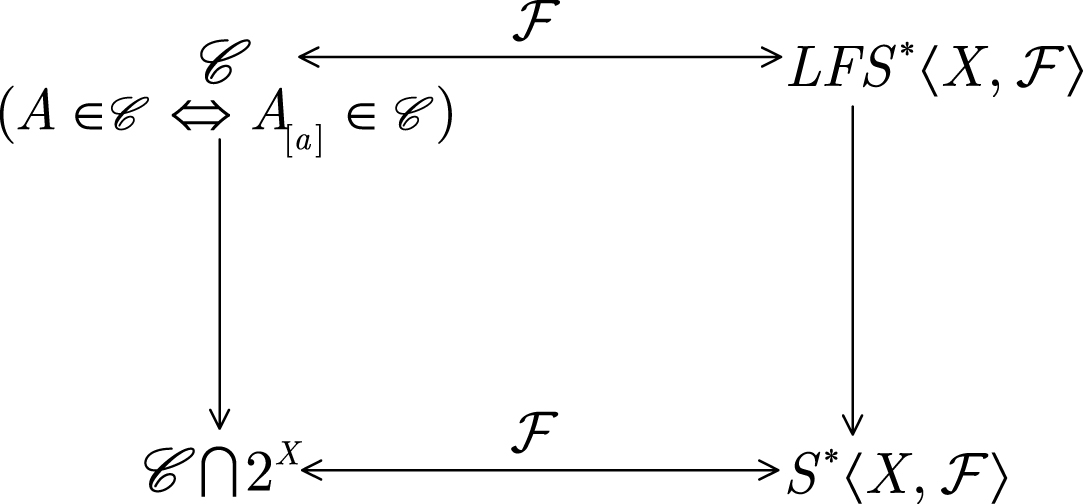
Theorem 4.10. If C is an induced L-convexity on X, then there exists an algebra 〈 X , F 〉 of type F such that C = LFS * 〈 X , F 〉 .

Proof. Firstly, it follows immediately from Lemma 4.8 (1) that C = C ∩ 2 X is a convexity and co C ( A ) = co C ( A ) for all A ∈ 2 ^X . Then we can construct an algebra 〈 X , F 〉 of type F in the same way of Lemma 4.9.

To prove C ⊆ LFS * 〈 X , F 〉 , it suffices to show that co C LFS * ( A ) ≤ A for all A ∈ C . If A = χ_∅, it is straightforward. If A ¬ = χ_∅, by Theorem 3.10, then co C LFS * ( A ) ( x ) = sg L ( A ) ( x ) = ⋁ k = 0 ∞ E k ( A ) ( x ) for all x ∈ X, where E⁰ (A) (x) = A (x) and E k + 1 ( A ) ( x ) = E k ( A ) ( x ) ∨ ( ⋁ { E k ( A ) ( x 1 ) ∧ ⋯ ∧ E k ( A ) ( x n ) | ∃ n ∈ ℕ , f F , x ˜ ∈ F n , x 1 , . . . , x n ∈ X , x = f F , x ˜ ( x 1 , . . . , x n ) } ) for each k ∈ ℕ . Combining this with the results of Lemma 4.8, it is easy to see that E (A) ≤ A. In a similar way, we obtain E ^k  (A) ≤ A for each k ∈ ℕ . So co C LFS * ( A ) ≤ A . Hence C ⊆ LFS * 〈 X , F 〉 .

On the other hand, by Lemma 4.9 and the construction of F , it is clear that S * 〈 X , F 〉 = C ∩ 2 X . For any A ∈ LFS * 〈 X , F 〉 , by Theorem 3.4, we know A [ a ] ∈ C for each a ∈ L. Since C is induced, we have A ∈ C . Hence LFS * 〈 X , F 〉 ⊆ C . □

Therefore, we can obtain the following diagram (see Fig. 1).

OPEN IN VIEWER

Fig.1

The relationship between L-subuniverses and L-convexities.

In this paper, the concept of L-subuniverses of an algebra 〈 X , F 〉 was introduced and their characterizations and representations were given. Besides, the relationship between L-subuniverses and L-convexities was discussed and it is shown that there is a one-to-one correspondence between L-subuniverses with the smallest L-subset and induced L-convexities.

As we have seen, an algebra 〈 X , F 〉 includes so many examples, such as a lattice, a group, a ring and so on. In the future, we will generalize the concept of L-subuniverses. We shall give some degree to which an L-subset is an L-subuniverses and discuss the relationship between L-subuniverse degrees and (L, M)-convexities.